
Cyber Risk Assessment of Transmission Lines in Smart Grids

1
College of Electrical Engineering, Chongqing University, Chongqing 400044, China
2
College of Electrical Engineering, Jinan University, Guangzhou 510632, China
3
College of Electrical Engineering, Illinois Institute of University, Chicago, IL 601106, USA
*
Author to whom correspondence should be addressed.
Energies 2015, 8(12), 13796-13810; https://doi.org/10.3390/en81212393
Submission received: 22 October 2015
/
Revised: 26 November 2015
/
Accepted: 27 November 2015
/
Published: 4 December 2015
(This article belongs to the Special Issue Decentralized Management of Energy Streams in Smart Grids)
Abstract
:The increasing use of information technologies in power systems has increased the risk of power systems to cyber-attacks. In this paper, we assess the risk of transmission lines being overloaded due to cyber-based false data injection attacks. The cyber risk assessment is formulated as bilevel optimization problems that determine the maximum line flows under false data injection attacks. We propose efficient techniques to reduce the computation complexity of solving the bilevel problems. Specifically, primary and secondary filtering techniques are employed to identify the lines whose flows will never exceed their limits, which can significantly reduce computation burden. A special feasibility cut-based acceleration technique is introduced to further reduce the computation burden. The simulation results on the IEEE 30-bus, IEEE 118-bus, IEEE 300-bus and IEEE 2383-bus systems verify the proposed risk assessment model and the effectiveness of the proposed filtering and acceleration techniques.
1. Introduction
Power systems are evolving to a large man-made Cyber-Physical System (CPS), whose reliable operation is crucial to a nation’s economy and homeland security. Supervisory Control and Data Acquisition (SCADA) systems are widely used by utilities for the communication between remote infrastructures and the control center. With the integration of more information technology, SCADA systems have evolved from using proprietary protocols and software to using open standards products and solutions including standard PCs and operating systems, Transmission Control Protocol/Internet Protocol (TCP/IP) and Ethernet communications and Internet access. Consequently, SCADA systems are becoming the primary target of cyber-attacks. It has been shown that an attacker can compromise the Direct Current (DC) state estimation by launching false data injection attacks, which could be undetectable if the attacker can construct the false data that obeys Kirchhoff’s Current Law (KCL) and Kirchhoff’s Voltage Law (KVL) based on the full network information of the power grid [1].
During the last six years, a lot of attentions have been directed to the study of cyber security in smart grids, with a focus on investigating the attacking mechanisms of false data injection attacks and the impact on the operation of power systems. Ozay et al. [2] proposed a distributed attacking strategy for false data injection attacks. The sparse optimization technique was used to construct the corresponding sparse attacking vector. Qin et al. [3] introduced the concept of unidentifiable attack, where the control center can detect the existence of false data but has no way to identify which meters are attacked. Xie et al. [4] investigated the impacts of false data on the real-time Locational Marginal Price (LMP) and analyzed the sensitivity of LMPs to injected false data. Ye et al. [5] proposed an assessment model for evaluating the potential risk of distribution automation systems to cyber attacks. More research work regarding false data injection models are presented in [6,7,8,9,10,11,12,13].
Note that there is a strong condition in [1,2,3,4,5,6,7,8,9,10,11,12,13] that the full network information of a power network is assumed to known to an attacker. This strong condition would make the proposed attacking model impractical. This might be beneficial to a defender. However, our previous work [14] revealed that the strong condition can be relaxed. In fact, an attacker only needs to obtain the network information of the attacking region to construct an undetectable attack vector based on KCL and KVL. The principle is to ensure that the incremental phase angles of all the boundary buses in the attacking region are the same such that the additional power flow due to the injected false data will never flow out the attacking region. As a result, the network information of the non-attacking region is not required. We also developed a heuristic algorithm [15] to determine a feasible attacking region for attacking the measurement at a load bus.
The physical security of lines has been widely recognized [16,17]. Recently, the cyber security of transmission lines has attracted much attention. Kim et al. [18] proposed a topology attack model. It was shown that the real-time topology sent to the control center can be masked by injecting a pair of false power injections at the terminal buses of the line to be attacked. To overcome the practical issues of the proposed model in [18], we introduced a local topology attack model [19], which determines an optimal attacking region for attacking a single line. A heuristic algorithm was proposed to minimize the effort of obtaining the network information. In [20,21], the authors further showed that some lines might be physically overloaded after the security constrained economic dispatch (SCED) due to cyber attacks. This is because SCED is performed according to the corrupted load data rather than the true load data. Accordingly, the calculated line flow is not the same as the true line flow. Thus, the line will be overloaded if its true flow is greater than the calculated flow that is limited within its flow limit. It is well known that the overloading of lines will pose a high risk on the reliable operation of power systems. The outage of a set of critical lines could lead to cascading failures, which would result in serious damages to power systems. For the safety of operation, it is essential for the operator to asset the risk of cyber-attacks: which lines could be overloaded due to the injected false data after SCED. These lines should be monitored and protected to avoid potential adverse impacts due to cyber-attacks.
In this paper, we assess the risk of transmission lines under cyber-attacks. The goal is to identify a set of lines that could be overloaded due to injected false data after SCED. The main contributions of this paper are three-fold:
- (1)
- We formulate the cyber risk assessment of transmission lines as a bilevel optimization problem. In the lower level, the SCED is performed to minimize the operation cost according to the received corrupted data. In the upper level, the power flow of a line is maximized to determine the cyber risk due to injected false data. The bilevel problem for each line is further transformed into an MILP problem.
- (2)
- We propose two fast filtering techniques to identify the lines whose flows will not exceed their flow limits under cyber-based false data injection attacks. This is based on the fact that there are few lines of which power flows may exceed the transmission limits due to the disruption of false data. This will reduce the computation burden of the risk assessment significantly by reducing the number of MILP problems that need to be solved.
- (3)
- We introduce a special feasibility cut to accelerate the solution process of the MILP problems. The special feasibility cut can significantly reduce the search space of the branch and bound algorithm for solving the MILP problems, so the computational burden is further reduced.
The rest of this paper is organized as follows: Section 2 reviews the concept of false data injection attacks. Section 3 presents the proposed model to assess the cyber risk of transmission lines, as well as the primary and secondary filtering techniques and the feasibility cut acceleration technique. Section 4 demonstrates the proposed risk assessment model and the effectiveness of the proposed filtering and acceleration techniques using the IEEE 30-bus, IEEE 118-bus, IEEE 300-bus and IEEE 2383-bus systems. Section 5 concludes the paper.
2. Review of False Data Injection Attacks
In a real-world power system, it is essential for the operator to obtain the real-time state of the system to monitor the operation and take preventive/corrective controls if necessary. To achieve the goal, a large amount of real-time measurements including line flow measurements, bus voltage measurements, and bus power injection measurements are transmitted to the control center to estimate the state of the system using the least-square method or other methods. In DC state estimation, the state is generally estimated by the least square method (1), where is the vector of measurements, is the vector of system state, and is the constant Jacobian matrix.
The accuracy of the received data could be compromised by the faults of sensors and other natural or malicious disruptions. Since the economic dispatch and other controls rely on the accurate result of the state estimation, so the operator will check the validity of the data by calculating the residual using (2) based on the estimated state
If is greater than the given threshold value, then some data is regarded as being corrupted. Unfortunately, this detection approach cannot ensure the integrity of the data transmitted to the control center. It has been shown in [1] that a wise attacker can construct the coordinated false data to avoid being detected by the residual checking. Thus, such an attack is called undetectable false data injection attack.
However, the attack model in [1] requires an attacker to obtain the network information of the entire power grid. If this is the real case, the risk of power systems to cyber-attacks will be mitigated significantly. This is because in practice it is very difficult for an attacker with limited budget to have this information since: (1) most power grids have thousands of buses and lines; and (2) power grid data are strongly protected. Unfortunately, we have proven that an attacker is able to construct an undetectable attack vector with incomplete network information [14]. This is done by ensuring that all boundary buses in the attacking region connected to the same non-attacking region have the same incremental phase angle. By doing so, the attacker only needs to obtain the topology and line parameters in the attacking region. A heuristic algorithm was proposed to obtain the feasible attacking region for attacking the measurement at a bus [15]. It was shown that an attacker only needs to have the network information of a small region to launch a successful attack. This observation indicates power systems are subject to a high risk of such attacks since a weak attacker can still attack the power system without paying a high cost. This also motivates us to assess the cyber risk of power systems, which will be addressed in the next section.
3. Mathematical Formulation of Cyber Risk Assessment Model for Transmission Lines
In this section, we propose the mathematical model for determining the maximum flow of a line under false data injection attacks. Several filtering and acceleration techniques are proposed to speed up the solution process.
3.1. Mathematical Formulation of the Bilevel Attack Model
In the real-time operation of power systems, when loads at buses change, the operator in the control center will redispatch the power outputs of units to achieve a new optimal operating point based on the data sent from a set of installed sensors. The power flows of lines are enforced within their flow limits for the purpose of reliable operation. Due to the close association with communication networks, Reference [20] pointed out that an attacker can inject false data into the measurements at load buses to change the readings sent to the control center. We further showed that an attacker can also launch a robust attack strategy even though the dispatch result of SCED is uncertain in the context of multiple solutions of SCED [21]. These corrupted data will induce the operator to make a false SCED which results in some lines being overloaded. From the perspective of system security, it is essential for a defender to determine these lines whose power flows can exceed their flow limits after SCED. This is done by calculating the maximum line flows due to false data injection attacks. These lines are viewed as high-risk lines due to cyber-attacks and should be strongly monitored to ensure the reliability and safety of power systems. The optimization problem of determining the maximum line flow is formulated as a bilevel optimization problem Equations (3)–(14):
subject to:
subject to:
The upper level of the above bilevel problem simulates the attacker’s attacking strategy, which is to determine the injected false data that maximizes the potential flow of line in Equation (3). The lower level simulates the system operator’s operation strategy, which is essentially an SCED problem that minimizes the total generation cost and load shedding cost in Equation (9). Constraint Equation (4) finds the absolute value of the flow for line . They can be modeled as Equations (15) and (16) below.
Constraint Equation (5) gives the line power flows after attacks. Note that the injected false data is not included since it is not a physical load. The amount of load shedding at a load bus is limited by the physical load in Equation (6). The injected false data is summed to zero in Equation (7) and the attacking amount at a load bus is limited by constraint Equation (8). Corresponding Lagrangian multipliers are assigned for power balance in Equation (10), line flow constraint Equation (11), and lower and upper bound constraints of generation in Equation (12), line flow in Equation (13), and load shedding in Equation (14).
Figure 1 summarizes the bilevel model for assessing the risk of one transmission line. In the upper level, an injected false data vector is determined to maximize the flow of a line after SCED. If is greater than the flow limit of line , then this line can be regarded as a high-risk line under cyber attacks. In the lower level, the operator minimizes the operation cost under the injected false load data . The risk assessment will be done for each transmission line, which means the bilevel problem will be solved multiple times. As shown later, solving the bilevel problem is a time-consuming process. This paper proposes two filtering techniques so that the bilevel problems for some lines can be skipped. This paper also proposes one acceleration technique so that the bilevel problems for the remaining lines can be solved faster.
Figure 1.
Bilevel model for assessing the risk of a transmission line.

3.2. Solution to the Bilevel Risk Assessment Model
In this section, we provide the solution to the bilevel optimization problem Equations (3)–(14). One of the most popular methods used to solve a bilevel optimization problem is the Karush-Kuhn-Tucker (KKT) based reformulation approach, in which the lower level is replaced with its KKT optimality constraints.
First, the lagrangian function of the lower level optimization problem Equations (9)–(14) is written as Equation (17):
At the optimal point, the first order optimality must be met, so we have:
According to the KKT optimality condition, the complimentary conditions for the inequality constraints Equations (12)–(14) should be also satisfied, which yields:
The nonlinear constraints in Equations (21)–(23) can be convert to the following linear constraints in Equations (24)–(26) using the big-M method [22].
where are diagonal matrices with all entries equal to . For each nonlinear constraint, two additional binary variables are introduced to linearize the complementary constraints and form the so-called big-M constraints. For instance, constraint Equation (24) is the linearized big-M constraints for constraint Equation (12). Similarly, Equation (25) is for Equation (13), and Equation (26) is for Equation (14). Constraint Equation (27) represents that the Lagrangian multipliers for inequality constraints should be non-negative.
Then, the lower optimization problem Equations (9)–(14) can be equivalent to the constraints in Equations (10)–(14), (18)–(20) and (24)–(27). Note that the objective function in the lower level has been removed. Accordingly, the bilevel problem in Equations (3)–(14) is transformed into an equivalent single-level MILP problem in Equation (28).
subject to Constraints Equations (5)–(8), (10)–(16), (18)–(20), and (24)–(27).
It is well known that the introduction of binary variables and the big-M constraints will increase the computation burden significantly. Thus, it is necessary to develop effective techniques to reduce the computation burden. It seems that we need to calculate the maximum flow by solving Equation (28) for each line. Luckily, in real power systems, most transmission lines will not be operating at or close to their flow limits. Accordingly, only a small number of lines may have flows exceeding their flow limits even under the disruption of false data injection. This motivates us to develop techniques to filter out those lines whose flows will never exceed their flow limits. In this paper, we propose two filtering techniques as described in the next two sections.
3.3. Primary Filtering Technique
It can be seen from Equation (5) that the line flow is determined by the generation vector and load shedding vector . This motivates us to initially determine the maximum line flows by only considering the power balance equation in Equation (10), the upper and lower bound constraints Equation (12) for , and the upper and lower bound constraints in Equation (6) for . Since the power flow of a line could be positive or negative, the maximum flow of line can be determined by solving the two LP problems introduced as follows:
subject to Constraints Equations (6), (10) and (12):
subject to Constraints Equations (6), (10) and (12).
We define . Then, the optimization problems in Equations (29) and (30) can be rewritten as Equations (31) and (34), respectively.
subject to:
where
subject to Constraints Equations (32) and (33).
Reference [23] showed that the optimal solutions to the above two LP problems can be obtained directly without actually solving the LP problems. In this paper, we employ this technique to determine the values of and . Without loss of generality, we assume that . Then there must exist an index such that:
Then, it is trivial to prove that:
Similarly, for the optimization problem Equation (34), there must exist an index such that:
Then, it is trivial to prove that:
The maximum flow of line k will be . This indicates that the maximum flow of a line can be directly calculated without actually solving the two LP problems. Thus, the computation burden will be reduced significantly. As only partial constraints of the optimization problem in Equation (28) are included, y is no less than the value determined by Equation (28) since the feasible region is enlarged. This indicates if , then the true maximum flow of line must be less than its flow limit; accordingly, this line can be excluded from further consideration. As a result, the number of MILP problems in Equation (28) to be solved is reduced by one.
3.4. Secondary Filtering Technique
As only partial constraints are included in the primary filtering phase, there might be a large difference between the calculated and true maximum line flows. In other words, the maximum flows of some lines would decrease significantly if all constraints in Equation (28) are included. This indicates that the primary filtering phase might not effectively filter out a large number of lines. Regarding this, we employ the secondary filtering technique to further filter out a subset of lines by narrowing down the feasible region in the primary filtering phase. As shown in Figure 2, suppose that the feasible region in the primary filtering phase is . To make the calculated maximum line flow closer to the actual value, we include all the primal constraints. Accordingly, the feasible region is narrowed to , the optimization problems in Equations (29) and (30) become Equations (39) and (40), respectively.
subject to Constraint Equations (6)–(8) and (10)–(14):
subject to Constraint Equations (6)–(8) and (10)–(14).
Figure 2.
Feasible regions of the primary filtering phase and the secondary filtering phase .

Note that Equations (39) and (40) are two LPs, which require much less effort to obtain the solutions compared to the KKT based MILP problem Equation (28). Thus, for the remaining lines that cannot be filtered out in the primary filtering phase, we solve two LP problems in Equations (39) and (40) in the secondary filtering phase. If the maximum flow of a line obtained based on Equations (39) and (40) is smaller than its line flow limit, then this line can be excluded from further consideration. As a result, the number of MILP problems in Equation (28) to be solved is reduced by one.
3.5. Acceleration via Feasibility Cut
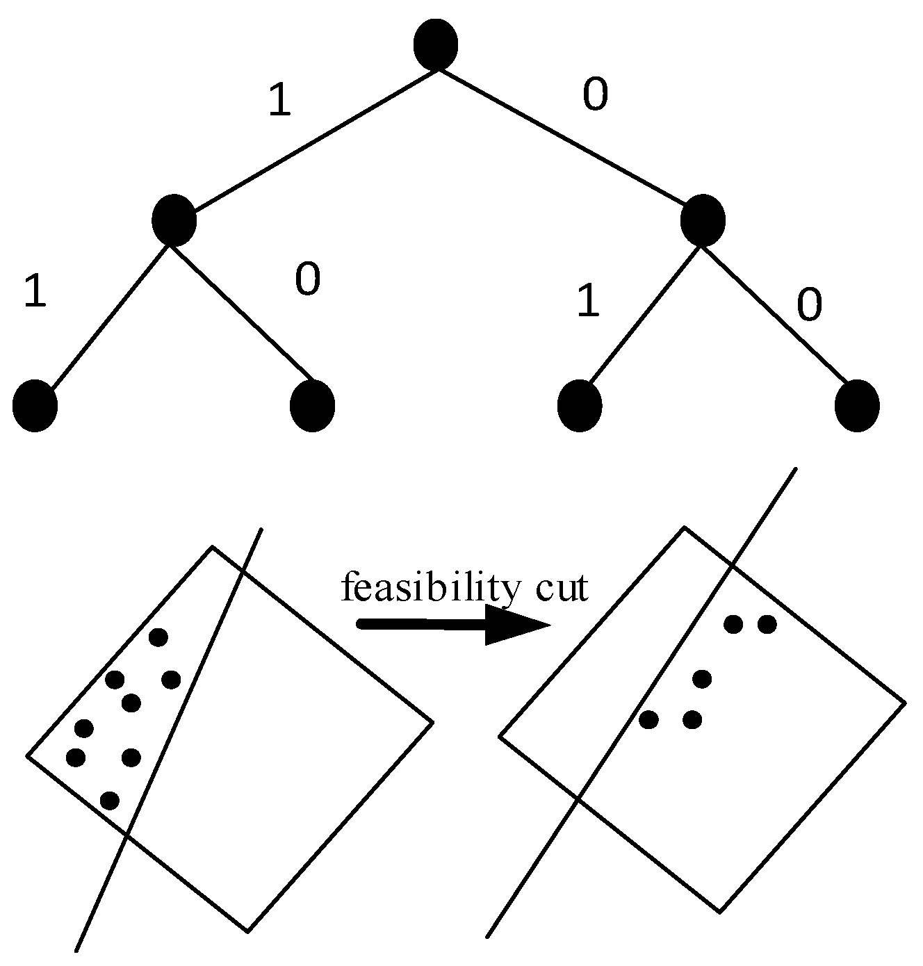
Note that Equation (28) is an MILP problem, which can be solved by the popular branch and bound algorithm. In essence, the branch and bound algorithm is an implicit enumeration algorithm. The advantage over the general enumeration algorithm is that it discards a large part of the search space based on the current estimate of the optimization problem. As shown in Figure 3, the basic principle of the branch and bound algorithm can be represented as a search tree. At each node, a branching rule is used to divide the feasible region into two or more subregions. For a given subregion, a bounding function is provided to determine a lower bound for the optimal solution for the entire feasible region. By doing so, the subregions in which the objective values are greater than the lower bound can be discarded, thus, the search space can be reduced.
Figure 3.
Principle of feasibility cut acceleration technique.

Note that the interest of a defender is to determine the set of lines whose flows will exceed their flow limits. The actual values of the line flows are not needed, especially for the lines whose flows will never exceed their flow limits after SCED. In light of this, we introduce an additional constraint Equation (41) into the optimization problem in Equation (28), which is to check whether the maximum flow of a line exceeds its limit rather than obtain the actual value of the maximum line flow.
Since satisfying Equation (41) means the optimization problem will have a feasible solution, we call Equation (41) a feasibility cut. Accordingly, adding Equation (41) is called the feasibility cut acceleration technique. The feasibility check problem is formulated as follows:
subject to Constraints Equations (5)–(8), (10)–(16), (18)–(20), (24)–(27) and (41).
Then, two cases are considered as follows.
Case 1: the maximum flow of line is less than its flow limit. In this case, Equation (42) is infeasible. That is, the branch and bound search process will stop after a finite number of iterations. Simulations show that the number of iterations with the feasibility cut is much less than that without the feasibility cut. This is because, as shown in Figure 3, the feasibility cut makes the feasible region an empty set, thus, the search space in the branch and bound algorithm can be reduced significantly.
Case 2: the maximum flow of line is no less than its flow limit. In this case, Equation (42) is feasible. That is, a feasible solution can be found after a finite number of iterations in the branch and bound search process. Note that, as shown in Figure 3, the feasible region is reduced if we introduce the feasibility cut, which reduces the search space of the branch and bound algorithm. In addition, since only the feasibility is checked, it requires less time than does the determination of the actual maximum line flow. This is because we only need to find one feasible solution. However, all feasible solutions have to be evaluated to determine the maximum flow.
Therefore, the introduction of the feasibility cut can reduce the computation complexity for both cases, especially for case 1. The advantage will be demonstrated in the case study.
4. Case Study
In this section, we first test the proposed risk assessment model using the IEEE 30-bus system, which has 30 buses and 41 lines. All the data are from MATPOWER 4.1 [24]. For the purpose of illustration, bus loads are scaled by 1.5. Simulations are carried out on a 2.4 GHz personal computer with 4 GB of RAM. We assume that an attacker has the full network information of a power grid. That is, the attacker has the full topology, line parameter, and bus load information. We also assume that the attacker can attack all the load measurements of the power grid. For simplicity and without loss of generality, the maximum allowable attacking amount at a bus is set to 50% of its load. The specific value of the threshold will not change the nature of the model, and can be easily modified in practical implementations.
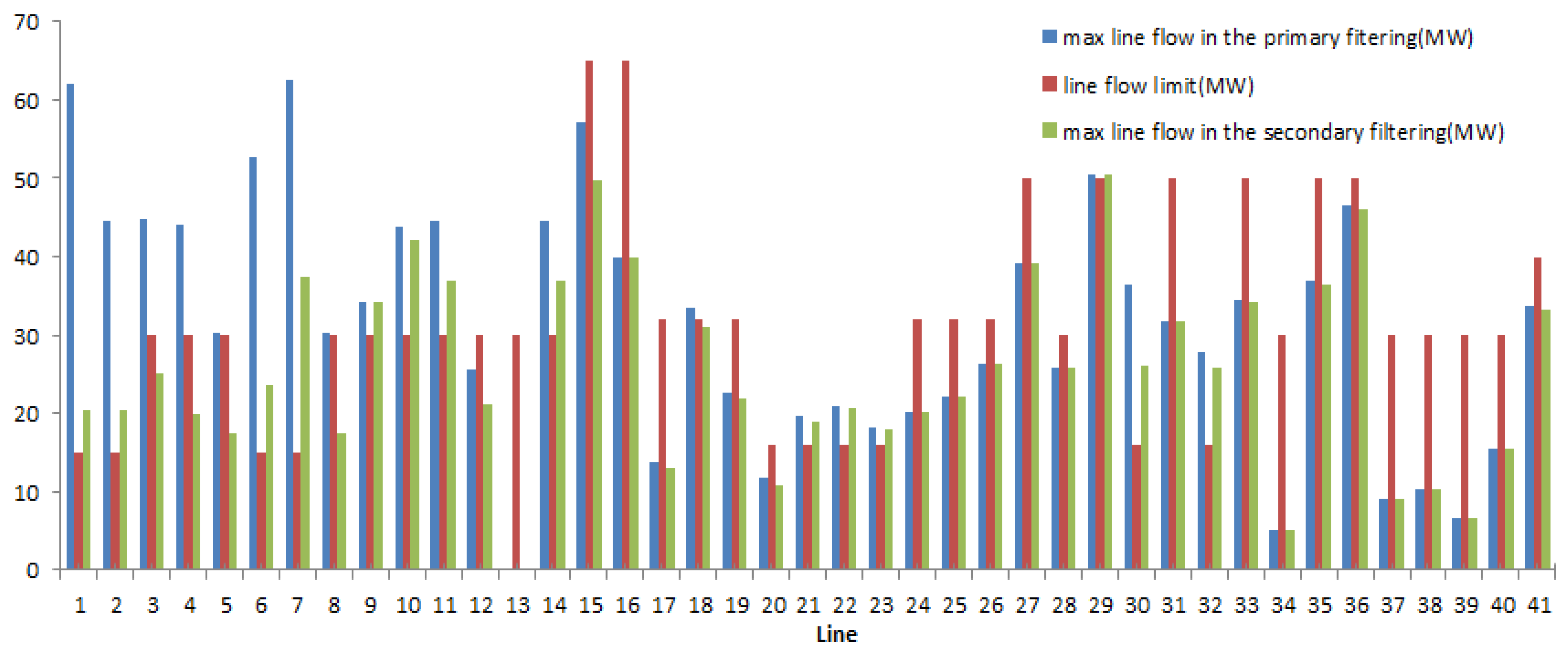
Figure 4 gives the maximum line flows determined in the primary filtering phase and the secondary filtering phase. It can be seen that the maximum flows of 22 lines determined in the primary filtering phase are less than their flow limits. That is, more than half of the lines are filtered out in the primary filtering phase and can be ignored in the secondary filtering phase. As mentioned, the primary filtering phase only includes partial constraints, so it can only provide rough upper bounds of the maximum line flows since the feasible region is enlarged. The true maximum line flows after SCED are smaller than the rough upper bounds. Thus, whether the true maximum flows of the remaining lines exceed the limits are unknown.
Figure 4.
Maximum line flows in the primary and secondary filtering phases.

Hence, in the secondary filtering phase, we further determine the maximum flows of the remaining lines. Compared to the primary filtering phase, we include all the primary constraints in the optimization problem in the secondary filtering phase. As shown in Figure 4, the maximum line flows are less than the values determined in the primary filtering phase. For instance, the maximum flow of line 1–2 determined in the secondary filtering phase is 20.30 MW, much less than 61.96 MW calculated in the primary filtering phase. This is because the line flow constraints in Equations (11) and (13) are introduced in the secondary filtering phase, which reduces the feasible region. Thus, the objective value is decreased and becomes closer to the true value. The secondary filtering phase determines that the flows of five lines, which cannot be filtered out in the primary filtering phase, are less than their flow limits. They will be excluded from next phases of the risk assessment.
In Table 1, and represent the maximum line flows determined by single-level MILP problem in Equation (28) with and without the feasibility cut in Equation (41), respectively. The term “infeasible” represents that Equation (28) with the feasibility cut is infeasible. That is, the maximum flow of a line after SCED will not exceed its flow limit. We can see that for lines 2–6, 4–6, 6–8 and 15–23 whose flows are greater than their flow limits, the maximum flows determined by the two models are the same. For the remaining lines, the maximum flows calculated by Equation (28) are less than their flow limits. This indicates that the introduction of the feasibility cut will not impact the determination of critical lines.

| Line index | From bus | To bus | (MW) | (MW) | Limit (MW) |
|---|---|---|---|---|---|
| 1 | 1 | 2 | infeasible | −7.29 | 15 |
| 2 | 1 | 3 | infeasible | 8.48 | 15 |
| 6 | 2 | 6 | 15.47 | 15.47 | 15 |
| 7 | 4 | 6 | 18.97 | 18.97 | 15 |
| 9 | 6 | 7 | infeasible | 21.05 | 30 |
| 10 | 6 | 8 | 34.41 | 34.41 | 30 |
| 11 | 6 | 9 | infeasible | −6.67 | 30 |
| 14 | 9 | 10 | infeasible | 3.55 | 30 |
| 21 | 16 | 17 | infeasible | 6.81 | 16 |
| 22 | 15 | 18 | infeasible | 15.98 | 16 |
| 23 | 18 | 19 | infeasible | 13.69 | 16 |
| 29 | 21 | 22 | infeasible | −41.53 | 50 |
| 30 | 15 | 23 | −20.10 | −20.10 | 16 |
| 32 | 23 | 24 | infeasible | 11.45 | 16 |
There are 41 lines for the IEEE 30-bus system, but only four lines 2–6, 4–6, 6–8 and 15–23 may be overloaded due to false data injection attacks. The objective of the risk assessment of transmission lines due to cyber attacks is to identify such a small set of critical lines. The injection of false data could make lines 2–6, 4–6, 6–8, and 15–23 overloaded although the SCED process in the control center aims to limit their line flows within their flow limits. This is because SCED is performed according to the corrupted load data, not the true load data. Accordingly, the calculated line flow is not the same as the true line flow. As an attacker can inject false data to make these lines out of service due to overloading after SCED, these lines are under high risk due to cyber-attacks. From the perspective of system security, it is essential for the defender to close monitor the operation of these lines.
Table 2 compares the iterations and run times of the branch and bound algorithm for the cases with and without the introduction of the feasibility cut in Equation (41). It can be seen that the iterations and run times are reduced if we introduce the feasibility cut, especially for the lines whose power flows are much smaller than their flow limits. For instance, the branch and bound algorithm needs 875,593 iterations and 25.94 s to determine the maximum flow of line 2–6. However, if constraint is added into the optimization problem in Equation (28), the iteration and run time are reduced to 88,676 and 1.33 s, respectively. For lines 9–10 whose maximum flow is much less than its limit 30 MW, the iterations is reduced from 479,843 to 159, and the run time is reduced from 7.91 to 0.05 s. This verifies the advantage of the introduction of the feasibility cut that it can effectively cut down the size of the search tree in the branch and bound algorithm and thus reduce the computation burden, especially for the case in which the line flow is less than the flow limit.
The run times for the primary and secondary filtering phases are 0.01 s and 1.32 s, respectively. In addition, it requires 12.80 s to determine the maximum line flows in Table 2. Thus, a total of 14.22 s is needed. However, if we do not consider the primary and secondary filtering techniques and the feasibility cut acceleration technique, the run time will be increased to 362.02 s, which is much higher than 14.22 s, the run time with the proposed filtering and acceleration techniques. It can be seen that the computational burden is reduced significantly by the primary and secondary filtering techniques and the accelerating technique in the branch and bound algorithm.
| Line index | From bus | To bus | Iterations | Run times (s) | ||
|---|---|---|---|---|---|---|
| Without feasibility cut | With feasibility cut | Without feasibility cut | With feasibility cut | |||
| 1 | 1 | 2 | 431,974 | 43,421 | 10.01 | 0.78 |
| 2 | 1 | 3 | 661,919 | 64,261 | 10.84 | 0.99 |
| 6 | 2 | 6 | 875,593 | 88,676 | 25.94 | 1.33 |
| 7 | 4 | 6 | 248,872 | 8279 | 4.29 | 0.31 |
| 9 | 6 | 7 | 303,782 | 36,367 | 5.68 | 0.69 |
| 10 | 6 | 8 | 302,966 | 13,059 | 7.74 | 0.36 |
| 11 | 6 | 9 | 315,716 | 142 | 8.30 | 0.55 |
| 14 | 9 | 10 | 479,843 | 159 | 7.91 | 0.05 |
| 21 | 16 | 17 | 422,800 | 23,227 | 7.05 | 0.61 |
| 22 | 15 | 18 | 134,188 | 86,674 | 3.06 | 1.34 |
| 23 | 18 | 19 | 147,809 | 51,190 | 3.23 | 0.83 |
| 29 | 21 | 22 | 294,511 | 195 | 8.27 | 0.27 |
| 30 | 15 | 23 | 269,026 | 136,799 | 5.87 | 2.51 |
| 32 | 23 | 24 | 338,603 | 113,257 | 8.72 | 1.87 |
The primary and secondary filtering techniques are also applied to the IEEE 118-bus system, which has 186 lines, the IEEE 300-bus system, which has 411 lines, and the Polish 2383-bus system, which has 2896 lines. Their effectiveness is summarized in Table 3, where is the load level coefficient. and give the number of lines filtered out in the primary and secondary filtering phases, respectively, and represents the ratio of the number of lines filtered out to the total number of lines. It is observed that fewer lines will be filtered out as the load level increases. However, there are still around 70% of lines filtered out by the filtering techniques when the system is under the load level . This shows the effectiveness of the proposed filtering techniques. In fact, most of power systems will not be operated at the very heavy load level for the reliable operation. The primary filtering phase can filter out most lines, but there are still a significant number of lines that can be filtered out in the secondary filtering phase. For instance, when , the secondary filtering phase will filter out 760 lines of the Polish 2383-bus system, around 1/4 of the total number of lines.
| ρ | IEEE 118-bus System | IEEE 300-bus System | Polish 2736-bus System | ||||||
|---|---|---|---|---|---|---|---|---|---|
| 0.6 | 143 | 21 | 88.17% | 273 | 48 | 78.10% | 2235 | 548 | 96.10% |
| 0.8 | 135 | 24 | 85.48% | 267 | 41 | 74.94% | 1964 | 667 | 90.85% |
| 1.0 | 128 | 19 | 79.03% | 259 | 43 | 73.48% | 1722 | 760 | 85.70% |
| 1.2 | 126 | 14 | 75.27% | 255 | 34 | 70.32% | 1541 | 824 | 81.66% |
| 1.4 | 119 | 14 | 75.51% | 245 | 33 | 67.64% | 1411 | 823 | 77.14% |
5. Conclusions and Future Work
The evolution of power systems into smart grids, while having great benefits, makes it possible for an attacker to design and inject false data into measurements that are sent to the control center, which may mislead the operator to perform a wrong SCED leading to the overloading of lines. In this paper, we propose a bilevel model to assess the cyber risk of transmission lines due to false data injection attacks. The results show that around 70% lines can be filtered out by the primary and secondary filtering techniques, which verifies the effectiveness of the filtering algorithm. For the remaining lines, the feasibility cut can significantly improve the efficiency of the KKT-based algorithm for determining the solution by reducing the feasible region.
Note that there are still a few lines where maximum flows are needed to be determined by solving the bilevel optimization problem Equations (3)–(14). However, thus far, there has been no an efficient algorithm to obtain the global optima of a bilevel optimization problem, especially for a large-scale system. To this end, one of our future works is to develop a fast algorithm to get a near-optimal solution to the bilevel problem.
As an extension of the work, we will also investigate the possibility of cascading failures triggered by false data injection, which represents a much more serious cyber risk for the system. The principle is that the outage of a small number of lines could trigger more line outages, especially when the system is under heavy load level. As a defender, it is essential to identify the set of critical lines whose outages can trigger cascading failures. To mitigate the risk of cascading failures, some countermeasures will be also expected to be developed.
Acknowledgments
This work is supported by the Fundamental Research Funds for the Central Universities (No. 0903005203358).
Author Contributions
Xuan Liu performed the experiments and wrote the paper, Xingdong Liu conceived the project, Zuyi Li reviewed and edited the manuscript. All authors read and approved the manuscript.
Conflicts of Interest
The authors declare no conflict of interest.
Nomenclature
| sufficient large number for Lagrangian multipliers | |
| sufficient large number for line power flows | |
| given small positive number for line flows | |
| given maximum percentage of change for loads | |
| number of loads/generators | |
| d, k | subscripts: index for loads/lines |
| load at bus d | |
| injected data into the measurement at bus d | |
| true power flow of line k | |
| calculated power flow of line k with injected false data | |
| transmission limit of line k | |
| number of lines filtered out in the primary filtering phase | |
| number of lines filtered out in the secondary filtering phase | |
| percentage of lines filtered out | |
| residual value | |
| absolute value of line flow | |
| Lagrangian multiplier | |
| coefficient for load level | |
| indicator variable for : if ; otherwise | |
| incremental phase angle at bus | |
| bus susceptance matrix | |
| Generation/load shedding cost vector | |
| bus load vector | |
| false data injection vector into load measurements | |
| true line flow vector | |
| calculated line flow vector with injected false data | |
| line flow limit vector | |
| incremental power flow vector | |
| Jacobian matrix | |
| load shedding vector | |
| generator power output vector | |
| , | generator maximum/minimum output power vector |
| shift factor matrix of the power grid | |
| bus-generator incidence matrix | |
| measurement vector | |
| Lagrangian multiplier | |
| indicator variables for Lagrangian multipliers |
References
- Liu, Y.; Ning, P.; Reiter, M.K. False data injection attacks against state estimation in electric power grids. ACM Trans. Inf. Syst. Secur. (TISSEC) 2011, 14, 21–32. [Google Scholar] [CrossRef]
- Ozay, M.; Esnaola, I.; Vural, F.T.; Kulkarni, S.R.; Poor, H.V. Sparse attack construction and state estimation in the smart grid: Centralized and distributed models. IEEE J. Sel. Areas Commun. 2013, 31, 1306–1318. [Google Scholar] [CrossRef]
- Qin, Z.; Li, Q.; Chuah, M.-C. Unidentifiable attacks in electric power systems. In Proceedings of the 2012 IEEE/ACM Third International Conference on Cyber-Physical Systems (ICCPS), Beijing, China, 17–19 April 2012; pp. 193–202.
- Xie, L.; Mo, Y.; Sinopoli, B. Integrity data attacks in power market operations. IEEE Trans. Smart Grid 2011, 2, 659–666. [Google Scholar] [CrossRef]
- Ye, X.; Zhao, J.; Zhang, Y.; Wen, F. Quantitative vulnerability assessment of cyber security for distribution automation systems. Energies 2015, 8, 5266–5286. [Google Scholar] [CrossRef]
- Mohsenian-Rad, A.-H.; Leon-Garcia, A. Distributed internet-based load altering attacks against smart power grids. IEEE Trans. Smart Grid 2011, 2, 667–674. [Google Scholar] [CrossRef]
- Hug, G.; Giampapa, J.A. Vulnerability assessment of AC state estimation with respect to false data injection cyber-attacks. IEEE Trans. Smart Grid 2012, 3, 1362–1370. [Google Scholar] [CrossRef]
- Kosut, O.; Liyan, J.; Thomas, R.J.; Lang, T. Malicious data attacks on the smart grid. IEEE Trans. Smart Grid 2011, 2, 645–658. [Google Scholar] [CrossRef]
- Giani, A.; Bitar, E.; Garcia, M.; McQueen, M.; Khargonekar, P.; Poolla, K. Smart grid data integrity attacks. IEEE Trans. Smart Grid 2013, 4, 1244–1253. [Google Scholar] [CrossRef]
- Kim, T.T.; Poor, H.V. Strategic protection against data injection attacks on power grids. IEEE Trans. Smart Grid 2011, 2, 326–333. [Google Scholar] [CrossRef]
- Rawat, D.; Bajracharya, C. Detection of false data injection attacks in smart grid communication systems. IEEE Signal Proc. Lett. 2015, 22, 1652–1656. [Google Scholar] [CrossRef]
- Dán, G.; Sandberg, H. Stealth attacks and protection schemes for state estimators in power systems. In Proceedings of the 2010 First IEEE International Conference on Smart Grid Communications (SmartGridComm), Gaithersburg, MD, USA, 4–6 October 2010; pp. 214–219.
- Wang, D.; Guan, X.; Liu, T.; Gu, Y.; Shen, C.; Xu, Z. Extended distributed state estimation: A detection method against tolerate false data injection attacks in smart grids. Energies 2014, 7, 1517–1538. [Google Scholar] [CrossRef]
- Liu, X.; Li, Z. Local load redistribution attacks in power systems with incomplete network information. IEEE Trans. Smart Grid 2014, 5, 1665–1676. [Google Scholar] [CrossRef]
- Liu, X.; Bao, Z.; Lu, D.; Li, Z. Modeling of local false data injection attacks with reduced requirement on network information. IEEE Trans. Smart Grid 2015, 6, 1686–1696. [Google Scholar] [CrossRef]
- Zhu, Y.; Yan, J.; Sun, Y.; He, H. Revealing cascading failure vulnerability in power grids using risk-graph. IEEE Trans. Parallel Distrib. Syst. 2014, 12, 3274–3284. [Google Scholar] [CrossRef]
- Hines, P.; Cotilla-Sanchez, E.; Blumsack, S. Do topological models provide good information about electricity infrastructure vulnerability? Chaos 2010, 3, 033122. [Google Scholar] [CrossRef] [PubMed]
- Kim, J.; Tong, L. On topology attack of a smart grid: Undetectable attacks and countermeasures. IEEE J. Sel. Areas Commun. 2013, 31, 1294–1305. [Google Scholar] [CrossRef]
- Liu, X.; Li, Z. Local topology attacks in smart grids. IEEE Trans. Smart Grid 2015. submitted. [Google Scholar]
- Yuan, Y.; Li, Z.; Ren, K. Quantitative analysis of load redistribution attacks in power systems. IEEE Trans. Parallel Distrib. Syst. 2012, 23, 1731–1738. [Google Scholar] [CrossRef]
- Liu, X.; Li, Z. Trilevel modeling of cyber attacks on transmison lines. IEEE Trans. Smart Grid 2015. [Google Scholar] [CrossRef]
- Fortuny-Amat, J.; McCarl, B. A representation and economic interpretation of a two-level programming problem. J. Oper. Res. Soc. 1981, 32, 783–792. [Google Scholar] [CrossRef]
- Zhai, Q.; Guan, X.; Cheng, J.; Wu, H. Fast identification of inactive security constraints in SCUC problems. IEEE Trans. Power Syst. 2010, 25, 1946–1954. [Google Scholar] [CrossRef]
- Zimmerman, R.D.; Murillo-Sánchez, C.E.; Thomas, R.J. MATPOWER: Steady-state operations, planning, and analysis tools for power systems research and education. IEEE Trans. Power Syst. 2011, 26, 12–19. [Google Scholar] [CrossRef]
© 2015 by the authors; licensee MDPI, Basel, Switzerland. This article is an open access article distributed under the terms and conditions of the Creative Commons by Attribution (CC-BY) license (http://creativecommons.org/licenses/by/4.0/).
Share and Cite
MDPI and ACS Style
Liu, X.; Liu, X.; Li, Z. Cyber Risk Assessment of Transmission Lines in Smart Grids. Energies 2015, 8, 13796-13810. https://doi.org/10.3390/en81212393
AMA Style
Liu X, Liu X, Li Z. Cyber Risk Assessment of Transmission Lines in Smart Grids. Energies. 2015; 8(12):13796-13810. https://doi.org/10.3390/en81212393
Chicago/Turabian StyleLiu, Xuan, Xingdong Liu, and Zuyi Li. 2015. "Cyber Risk Assessment of Transmission Lines in Smart Grids" Energies 8, no. 12: 13796-13810. https://doi.org/10.3390/en81212393