1. Introduction
In the past several decades, China’s power system has experienced rapid development along with rapid economic growth. Among all electric power sources, thermal power, which mainly consists of coal-fired plants, accounts for the largest proportion of China’s power system. By the end of 2012, China’s total installed generation capacity reached 1146.76 GW, of which 819.68 GW (approximately 71.5%) was from thermal power, and the total electric energy production reached 4986.5 TWh, with 3925.5 TWh (approximately 78.7%) coming from thermal power. Simultaneously, the utilization hours of the installed capacity for thermal power plants are larger than those of hydro power or wind power. The statistical results of 2012 showed that the annual utilization hours of power plants with an installed capacity over 6 MW are 4982 h for thermal power, 3591 h for hydropower and 1929 h for wind power [
1,
2,
3,
4,
5]. However, because the preheating and cooling of the stream-turbine requires more time than other resource units, the coal-fired thermal unit is inflexible between start-up and shut-down resulting in a slow response to system load demands. Moreover, the start-up and shut-down of coal-fired thermal units cause high fuel costs [
6,
7,
8,
9]. Generally, thermal plants are usually scheduled to meet base load demands to ensure that the generation process runs smoothly and reduce the start-up and shut-down times of thermal units. Furthermore, the different values of power system demand become larger among adjacent days due to various factors, including heavy weather, minor vacation, and transition periods between dry and wet season for hydro power [
10,
11]. This situation causes remarkable difficulties in preparing the generation schedule for power systems, especially for ones with numerous thermal plants. Consequently, the power dispatch centers of China are in charge of the medium-term optimal commitment of thermal units (MOCTU), which usually span from one month to half a year and take one day as the time interval in calculations to obtain the numbers and times of the start-up and shut-down units for every thermal plant each day before actual short-term and daily-ahead scheduling.
The objective of MOCTU is to find the optimal set of thermal generating units or the boot capacity (sum capacity of units that putting into operation in the first operation of a plant) scheme of a power system to satisfy the system load demand, operational restrictions, reliability constraints, and security requirements in each time period. Thus the MOCTU is a form of unit commitment (UC) problem [
8,
9,
12]. In contrast with short-term UC in power systems, which involves determining a start-up and shut-down schedule of units to meet the required demand during a short-term period such as one day or one week [
13,
14], MOCTU is responsible for dispatching load to each plant for maintenance scheduling and hydrothermal coordination. The main difference between medium-term and short-term thermal UC optimization is that medium-term optimization takes each plant’s operating capacity or unit numbers as decision variables instead of scheduling a single unit by short-term operation [
15]. It is well-known that the utilization rate of power generation equipment reflects the generation ability of a thermal plant, and the standby condition of generation equipment reflects the ability of a thermal plant to deal with sudden accidents, and utilization hours of the installed capacity for thermal power plants can reasonably reflect the two abovementioned factors, so that operators can operate and manage plants better. Hence, many power grids take equal accumulated operating hours of installed capacity for all thermal power plants as the primary objective of MOCTU during the selected period. However, due to thermal power’s main characteristics, including slow start-up and shut-down, complex constraints, large-scale as well as large complicated demands by power grid, developing and establishing computer simulation and optimization models for thermal UC optimization have been most challenging and complex issues [
16,
17,
18]. Furthermore, to achieve the best possible optimal solution and the largest benefit for thermal power plants and power grid, the model should be simulated as close to reality as possible to suit the practical needs of power dispatch centers, especially in China [
19,
20,
21]. However, according to our retrieval results, there are few studies on MOCTU, especially on the development of simulation models for MOCTU that meet the demands of practical engineering [
22,
23]. In this paper, a medium-term thermal UC optimization model with equal capacity utilization hours for all thermal power plants is established. The model not only respects the basic principles of electric power dispatch (equality, impartiality and transparency), but also adopts a reward principle that gives extra operation hours to the thermal plants with low energy consumption and dust discharge and high efficiency, namely reward hours.
The work described in this paper is originated from the real, practical demands for power dispatch centers of China to develop a medium-term optimal commitment of thermal units. The aim of this paper is to develop a simulation model for MOCTU to satisfy the needs of practical engineering and present a feasible and effective algorithm to optimize the model. MOCTU is a multi-stage decision problem that involves a highly nonlinear and computationally expensive objective function with a large number of constraints. The progressive optimality algorithm (POA) has been shown to be an effective method for solving multi-stage optimization problems by decomposing a multi-stage decision problem into a series of non-linear programming two-stage problems [
24,
25,
26,
27,
28], and it is suitable for solving MOCTU. However, it is a difficult task to find feasible solutions for a large-scale MOCTU problem using POA due to its drawback, namely the easily encountered local optimum for complex problems. Therefore, in this paper, an improved progressive optimality algorithm (IPOA) is proposed for a large-scale MOCTU problem with nine thermal plants and 27 units in Yunnan Province of China to validate the effectiveness and practicality of the developed simulation model as well as to improve the quality of optimal solutions of POA. The original optimization problem is first optimized by using a heuristic method and an initial feasible solution is obtained, then POA is adopted to search the optimal solution, and finally two strategies are utilized to adjust the solution from the constraint boundaries into the feasible zone’s interior to continue to search for the global solution. Actually, the mid-term boot scheduling plan of thermal plants has been generated by operators in Yunnan power grid (YNPG) using this proposed simulation model and method since 20 May 2013. Over a two-year implementation period, it has given operators more confidence to use it.
This paper is organized as follows:
Section 2 gives the formulation of the mathematical model of MOCTU;
Section 3 analyzes the characteristics of this problem and presents the IPOA used to solve it;
Section 4 applies the model to a real-world scenario with nine thermal plants and 27 units in Yunnan province of China; Finally,
Section 5 presents the conclusions.
3. Model Solution
3.1. Solution Approach
MOCTU is a form of the UC problem with a large number of constraints, including unit number constraints (Constraint Group 1), system power balance constraints (Constraint Group 2), peak and valley duration constraints (Constraint Group 3), and boundary condition constraints (Constraint Group 4). It is obvious that Constraint Groups 1 and 2 are single-period constraints that can be treated to reduce the search space. Although Constraint Groups 3 and 4 are multi-period constraints, Constraint Group 4 can be satisfied when Constraint Group 3 is satisfied in extended calculation periods. On the other hand, MOCTU is a high dimensional problem to be optimized. For a power grid with two thermal plants, each having three units. For one plant with three units, it has (3 + 1) kinds of combination in one period, and for two plants, it reaches (3 + 1)2, so the total number of unit combinations will reach [(3 + 1)2]30 1.3291036 for a horizon of one month with 30 periods, and the overhead of optimization will be computationally expensive. Considering the complex constraints, especially Constraint Group 3, the solving process can be divided into two procedures:
Procedure І: Obtaining the feasible solution space
, where
represents all of the possible unit-commit combinations that satisfy Constraint Groups 1 and 2 in period t. First, combine all units of all plants to obtain all possible unit-commit combinations in each period. Second, obtain the solution space
by filtering out the combinations that cannot satisfy Constraint Groups 1 and 2 period-by-period. The solution for the UC scheme in the calculation period can be acquired from the unit-commit combinations in
. The above process is relatively simple.
Procedure II: Search for the global optimal solution that can meet Constraint Group 3. Because the solution in
from Procedure І already satisfies Constraint Groups 1 and 2, and as well as Constraint Group 4 being automatically satisfied after satisfying Constraint Group 3, the aim of this search process is to find the solution that satisfies Constraint Group 3. The following discussion will introduce how to find the optimal scheduling that meets Constraint Group 3 in the solution space
. First, generate an initial feasible solution in
that satisfies Constraint Group 3 by using heuristic method. Second, produce the global optimal solution by the POA. However, POA is sensitive to initial trajectories and sometimes cannot guarantee a global optima, which is the reason that restricts its application. Thus, POA easily converges to a local optimum while being directly used for MOCTU, which is a strong constrained optimization problem. For the medium-term thermal UC optimization, a local optimum means that the system power reaches the upper or lower limit boundary constraints or that the duration periods of peak and valley in the operating capacity process are equal to the limit value of the minimum duration periods. In this case, it is very difficult to further optimize the result. Therefore, an improved POA combining POA with two adjustment strategies is presented to overcome the mentioned demerits.
3.2. Initial Feasible Solution Generation
As
Procedure І has achieved the solution space
that meets Constraint Groups 1 and 2, the initial feasible solution can be acquired by searching the solution space
by heuristic method only when the operating load rate approximates to the given target load rate that obtained from long-term schedule of power dispatch centers in each period. The feasible region in the latter period will be sharply contracted when the generating scheme in the previous period is determined and the duration period constraints (Constraint Group 3) are considered. To avoid the infeasible region, this paper suggests
as the target load rate. Before searching, sort the generating schemes in
in every period according to the ascending order of the index value
. Where
represents the operating load rate of the
kth generating scheme in
, and its formula is as follows:
The generating scheme
, which is sorted according to the ascending order of the index value
in every period, can be obtained by using Equation (10). Then, the feasible solution can be obtained from the sorted solution space
by the heuristic method. The detailed procedure is as follows:
- Step 1:
Construct an integer array ks of length T. Set ks[1] = 1 and t = 1. Make sure that the combination of boot capacity in period 1 is the first element of the solution space
.
- Step 2:
Set t = t + 1. If t > T, go to Step 6. Otherwise, set ks[1] = 1 and set the combination of boot capacity in period t as the first element of the solution space
.
- Step 3:
Verify whether the start-up mode lying in the interval of [0,1] satisfies the constraints of Equation (3). If it does satisfy them, go to Step 2; otherwise, go to Step 4.
- Step 4:
Set ks[t] = ks[t] + 1. If ks[t] is greater than the number of elements in solution space
, go to Step 5. If not, replace the combination of boot capacity in period t with the ks[t]th element of the solution space
and go to Step 3.
- Step 5:
Set t = t + 1, and go to Step 1.
- Step 6:
Output the result.
3.3. Optimization Process of Progressive Optimality Algorithm (POA)
Considering the complex requirements by power grids and the constraints mentioned above, the present optimization problem exhibits multi-stage, large-scale and high dimension characteristics. A suitable solution algorithm is required for solving the MOCTU. Based on Bellman’s Principle, the POA, which is proposed by Howson and Sancho for reducing dimensionality difficulties by decomposing a multi-stage decision problem into a series of non-linear programming two-stage problems [
29], has been shown to have great advantages over classical optimization methods as one of the most widely used techniques for hydroelectric generator scheduling and water resources problems [
30,
31]. The advantages of POA over other optimization techniques are that it can decompose a multi-state decision problem into several nonlinear programming sub-problems to reduce the dimensionality. More specifically, the merits of POA have clearly been elaborated in [
32], including no need to discretize the state variables, no resolution or linearization of nonlinear objective functions and constraints and minimal storage requirements.
To understand the main principle of POA, a general multi-stage optimization example was given. In this example, a set of state variables
is given to determine the optimal solution by minimizing objective functio
, where
and
are given as the initial state values. The algorithm starts with an initial trajectory
which is gained in a certain way. Then, this multi-stage decision problem would be decomposed into two problems, each of which minimizes
to obtain optimal
at stage
i during the
jth iteration by fixing values of
and
. In other words,
and
are fixed to optimize
to yield
, as shown in
Figure 2a. Then
and
are fixed to optimize
for
, as shown in
Figure 2b, in turn, the
jth iteration isn’t finished until
is obtained, as shown in
Figure 2c,d. Based on the optimized results from the last iteration, another iteration is restarted again. The process isn’t over until the difference between the last two iterations meets the predefined precision limit.
Figure 2 illustrates the optimization process during the
jth iteration.
Figure 2.
Optimization process of progressive optimality algorithm (POA).
Figure 2.
Optimization process of progressive optimality algorithm (POA).
The initial feasible solution obtained in
Section 3.3 is used for POA to search for optimal solution. The general process can be mainly described in the following steps:
- Step 1:
Set the generating scheme to an initial feasible solution generated by the heuristic search and an initial objective function value
. Set t = 1 and k = 1.
- Step 2:
Obtain a generating scheme by replacing the generating scheme in period t with the kth element of the solution space
. If the new generating scheme meets Constraint Group 3, go to Step 3. If not, go to Step 4.
- Step 3:
Calculate the objective function value
according to Equation (5). If
, adjust the results by using the equalization operation and combination operation and set
.
- Step 4:
Set k = k + 1. If k is greater than the number of elements in solution space
, go to Step 5. If not, go to Step 2.
- Step 5:
Set t = t + 1 and k = 1. If t < T, go to Step 2. If not, it means one iteration has been performed, then check whether the objective value has been improved over the previous iteration. If so, set the initial solution as the acquired result and go to Step 2. If not, go to Step 6.
- Step 6:
Output the result.
3.4. Equalization Operation and Combination Operation
Although possessing advantages of quick and strong convergence, POA easily falls into sub-optimal results because each iterative calculation is merely associated with a single period. Unable to make full use of the multi-stage information of the original problem, the sub-optimal results are easily attained at the bounds of constraints. To enhance the searching space and obtain the global optimal result, two strategies are presented including: equalization operation of the system operating capacity and single station boot peak combination operation.
The equalization operation of the system operating capacity is for making the start-up units’ capacity equal to the shut-down units’ capacity as much as possible by means of adjusting the ratio of the system load demand for each time and operating capacity to approach
. The equalization operation has two purposes: (1) to make the system generating scheme move from the power constraint boundary into the feasible solution’s interior; and (2) to make it more convenient to move and merge the peak of the operating capacity. The equalization process is equivalent to solving the following programming problem:
The constraints are the same as those we have previously mentioned. The approach needs to traverse the generating scheme of each plant in turn and to find whether it satisfies all constraints when performing start-up (shut-down) of one unit in period
t and shut-down (start-up) of one unit in period
. If it satisfies the constraints, the problem can be optimized with Equation (11) as the target. In the search process, the system’s operating capacity remains unchanged, and it can guarantee that the capacity utilization hours of every plant are unchanged. The search process is shown in
Figure 3.
Figure 3.
Sketch map of the system’s boot capacity equalization.
Figure 3.
Sketch map of the system’s boot capacity equalization.
As the equalization operation makes the start-up unit’s capacity equal to the shut-down unit’s capacity as much as possible, it provides the peak moving of a single plant’s operating capacity some space for adjustment. The single station boot peak combination process searches the single station boot capacity in turn for the peak with the minimum number of duration periods and finds whether it should move and merge it with other peaks. If so, it executes the combination operation. Without changing the objective function value, this method can make an adjustment to the operating capacity process, which requires that the operating durations of peak and valley periods equalize to the demanded minimum duration, and forces it to leave the local optimum. The peak combination operation is shown in
Figure 4.
Figure 4.
Sketch map of the single station boot peak combination.
Figure 4.
Sketch map of the single station boot peak combination.
From Equations (2)–(6), it can be seen that the installed capacity utilization hours of a thermal power plant is relative to the accumulative total but not the process of the scheme. Utilizing the two operations mentioned above, the results from POA can be converted by making the generating scheme move from the constraint boundary to the feasible region internal area under the condition of the unchanged objective function. As a result, POA acquires its new search space and will not stop iterating until convergence is obtained. The search principle of POA with the two strategies is shown in
Figure 5. The lines of
,
and
represent the isopleths of the objective function value. According to Equation (5), the objective function value is zero for the best solution
, namely
. Two main steps are defined in the optimization process. Step α is defined as the optimization process of POA and β presents the adjustment process of equalization operation and merge operation. First, the initial feasible solution
converges to the local optimal solution
through Step α which cannot be further optimized because
lies on the constraint boundary. Secondly, through Step β the local optimal solution
can be moved along the target isopleth
to
which is still in the feasible solution internal area, then step α is reutilized and solution
is obtained. If
still lies on the constraint boundary, then step β is utilized again and the local optimal solution
is moved along the target isopleth
to
. Based on the optimized results from the adjustment process, another iteration is restarted again until the global optimal solution
is obtained.
Figure 5.
Sketch map of the search principle.
Figure 5.
Sketch map of the search principle.
3.5. Solution Architecture
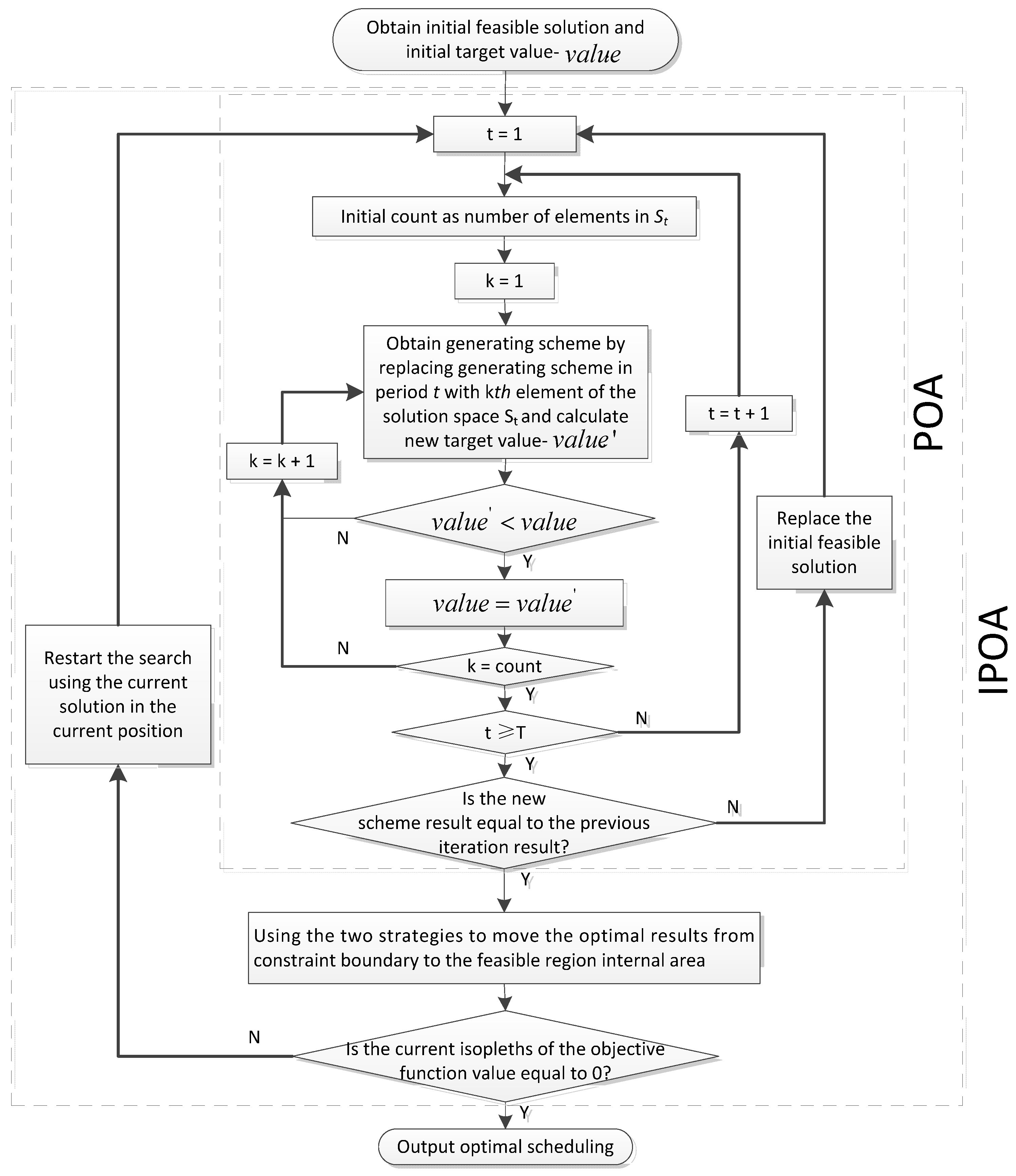
With a large amount of constraints and complex requirements, MOCTU is a challenging optimization problem that involves a highly nonlinear and computationally expensive objective functions. The optimization process is divided into two procedures: generation of an initial feasible solution and optimization of POA. However, POA is sensitive to initial trajectories and easily converges to local optima. Thus any changes from the decision or state variables may have a slight improvement on the solutions. Therefore, IPOA is adopted with the equalization operation and the combination operation to adjust the results acquired from POA. By doing this, it moves the solutions from constraint boundaries into the feasible zone’s interior and then continues to search for the optimal solution with POA. The solution flowchart of MOCTU is shown in
Figure 6 and the general process for the IPOA procedure can be mainly described in the following steps:
- Step 1:
Obtain the initial feasible solution by heuristic search and calculate the objective function ;
- Step 2:
Obtain the optimal results by using POA and calculate the objective function
(the detailed process is described in
Section 3.3);
- Step 3:
Judge whether the current isopleths of the objective function value are equal to zero, if not, use the two strategies to move the optimal results from the constraint boundary to the feasible region internal area to search again. Otherwise, go to Step 4.
- Step 4:
Output optimal scheduling.
Figure 6.
Solution flowchart of medium-term optimal commitment of thermal units (MOCTU) by improved progressive optimality algorithm (IPOA).
Figure 6.
Solution flowchart of medium-term optimal commitment of thermal units (MOCTU) by improved progressive optimality algorithm (IPOA).
4. Simulation Results
The proposed simulation model and method have been applied to the YNPG in China. Currently, it is used as the primary tool to determine the mid-term boot scheduling of thermal plants by the operators of YNPG. By the end of 2013, the total installed capacity of YNPG had reached 26.1 GW among which hydro power was responsible for 16.7 GW and thermal power was responsible for 8.935 GW. The reasonable scheduling of thermal power is beneficial for optimizing hydropower systems and system security.
The thermal power system in the YNPG consists of nine thermal power plants and 27 units. As mentioned above in
Section 3.3, it is a highly dimensional and complex problem to optimize. Therefore, it is a substantial challenge to determine the medium-term operating policies for these thermal plants. The dispatch center in the YNPG is in charge of these thermal power systems.
Table 1 lists the basic data of these plants. IPOA has been implemented in Java on a PC with an Intel
® Core™2 Duo CPU, operating at 2.93 GHz, with 2 GB of memory. A real scheduling for 2013 in the YNPG is used to test the validity and computational efficiency of the proposed method.
October, a typical month and the beginning of the dry season, was selected to demonstrate the actual availability of the simulation model as well as the practicality and efficiency of the method. In October, the hydro-power system comes to its lowest output and the demand on the thermal system increases. As a result, the operating scheduling of thermal power plants will obviously change. The simulation results and rationality of the algorithm will be presented in the paper. According to the real-world operating experience and users' actual demands, the parameters are set as follows:
- 1)
Given load rate of plant
, ;
- 2)
Minimum load rate of thermal power,
;
- 3)
Maximum load rate of thermal power,
;
- 4)
Minimum duration periods of peak in the operating capacity process of plant
during the calculation period,
;
- 5)
Minimum duration periods of valley in the operating capacity process of plant
during the calculation period,
;
- 6)
Maximum unit number of plant k in period t, set
as the number of installed units
- 7)
Minimum unit number of plant i in period t,
, except
while
;
- 8)
Actual capacity utilization hours of plant i in the pre-calculation period,
;
- 9)
Extra award hours of plant i,
;
- 10)
System load demands in each period and the first ten days’ boot process () are all given.
Table 1.
Thermal power system in Yunnan power grid (YNPG).
Table 1.
Thermal power system in Yunnan power grid (YNPG).
| Thermal plant | Units (number × capacity, MW) | Capacity (MW) |
|---|
| A | 4 × 600 | 2400 |
| B | 6 × 300 | 1800 |
| C | 4 × 300 | 1200 |
| D | 2 × 200 + 2 × 300 | 1000 |
| E | 2 × 300 | 600 |
| F | 2 × 300 | 600 |
| G | 2 × 300 | 600 |
| H | 2 × 300 | 600 |
| I | 1 × 135 | 135 |
Comparison of each power plant’s capacity utilization hours calculated by IPOA in October is shown in
Table 2.
Table 2.
Comparison of each power plant’s capacity utilization hours in October (h).
Table 2.
Comparison of each power plant’s capacity utilization hours in October (h).
| Items | Heuristic search | POA | First adjustment | IPOA |
|---|
| Plant A | 547.2 | 422.4 | 422.4 | 422.4 |
| Plant B | 297.6 | 416.0 | 416.0 | 422.4 |
| Plant C | 369.6 | 422.4 | 422.4 | 422.4 |
| Plant D | 240.0 | 422.4 | 422.4 | 422.4 |
| Plant E | 489.6 | 422.4 | 422.4 | 422.4 |
| Plant F | 489.6 | 432.0 | 432.0 | 422.4 |
| Plant G | 499.2 | 422.4 | 422.4 | 422.4 |
| Plant H | 528.0 | 432.0 | 432.0 | 422.4 |
| Plant I | 422.4 | 422.4 | 422.4 | 422.4 |
| Average value | 431.5 | 423.8 | 423.8 | 422.4 |
| Max-min difference | 307.2 | 16.0 | 16.0 | 0 |
| Objective value (h2) | 10283 | 23.0 | 23.0 | 0 |
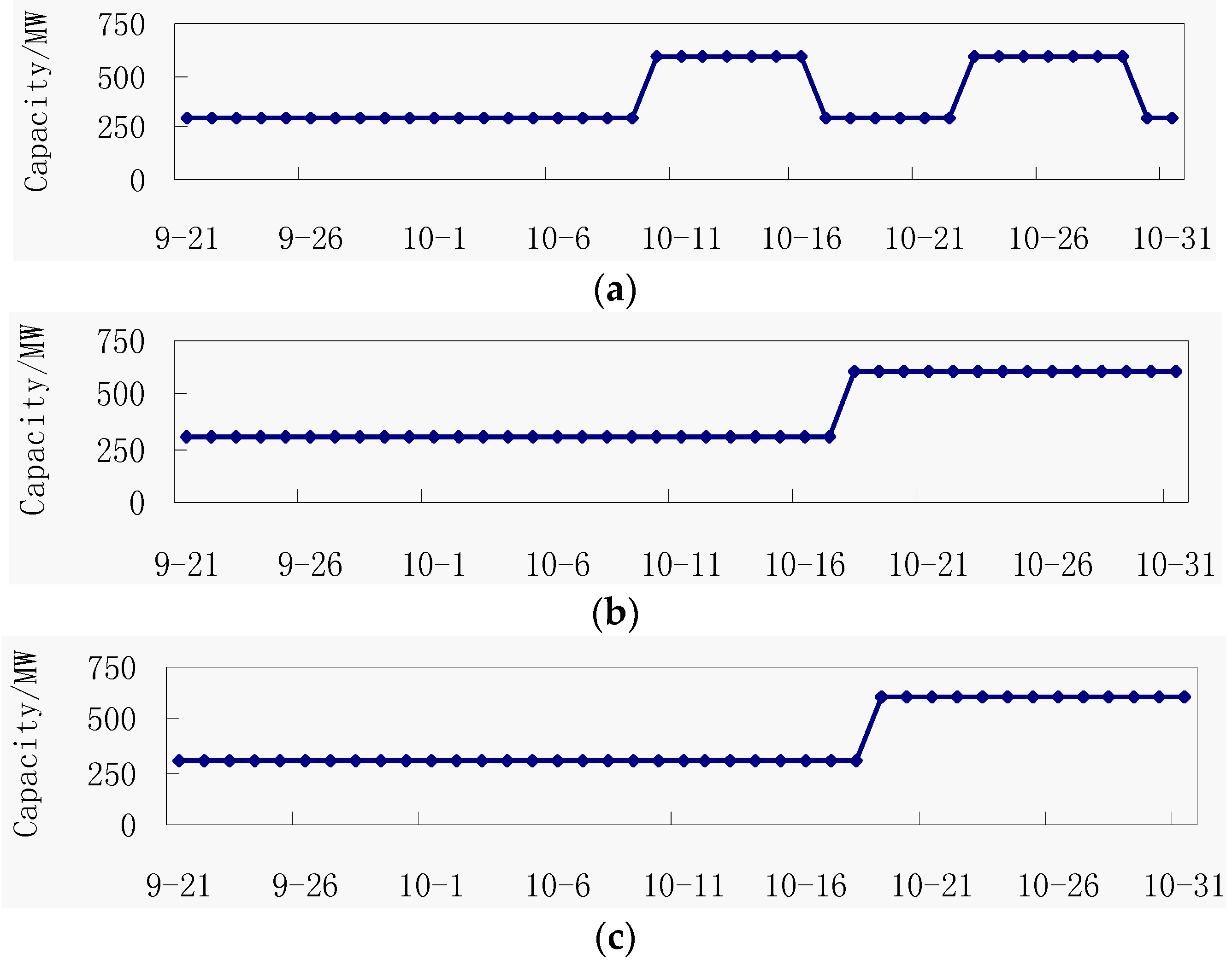
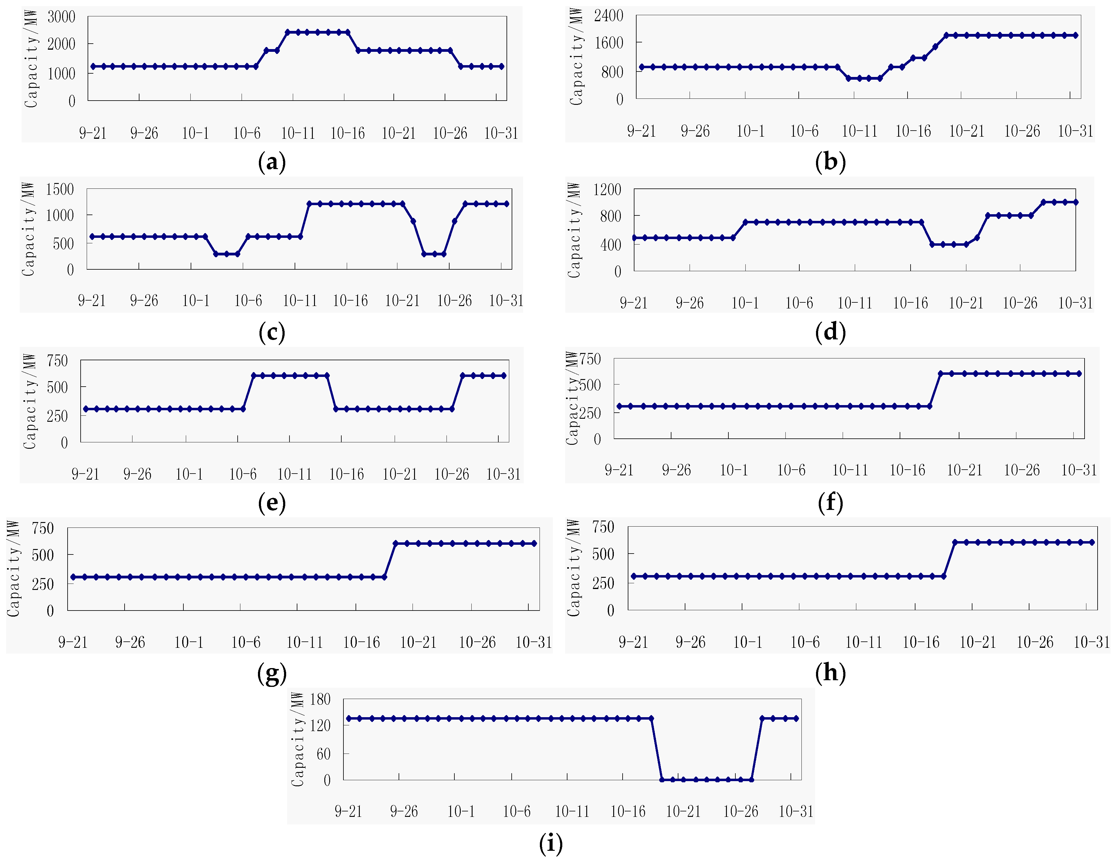
Figure 7 and
Figure 8, respectively, show system energy balance maps and boot modes of plant
F by different methods (the horizontal axis represents the time period). As can be seen from
Figure 7, the results of the simulation model match the actual characteristics of thermal power system in October that the load demand on the thermal system is increasing. It demonstrates that the proposed simulation model for MOCTU is very practical and can satisfy the actual project requirements.
Figure 7.
Energy balance maps by three methods: (a) POA; (b) first adjustment; (c) IPOA.
Figure 7.
Energy balance maps by three methods: (a) POA; (b) first adjustment; (c) IPOA.
Figure 8.
Boot capacity of Plant F for three methods: (a) POA; (b) first adjustment; (c) IPOA.
Figure 8.
Boot capacity of Plant F for three methods: (a) POA; (b) first adjustment; (c) IPOA.
The calculation results on the YNPG are shown in
Table 2. IPOA is compared with heuristics and POA. Max-min difference and objective value are taken as the measurement index. When the initial solution is obtained by heuristics, most plants’ capacity utilization hours are different. As shown in
Table 2, calculated by heuristic and POA in turn, the max-min differences are 307.2 h and 16 h, and the objective values are 10,283.0 h
2 and 23.0 h
2. Although the results have been significantly improved, the optimal solution is still not found. The reason is that the results obtained from POA run into local optima. The results by POA in
Figure 7a illustrate that it has reached the system’s power constraint boundary in many periods (10-08, 10-09, 10-30) and
Figure 8a shows that two peak values of Plant
F’s boot mode reach the duration periods of peak in the operating capacity constraint, and it cannot be optimized any further by POA.
Table 2,
Figure 7b and
Figure 8b show that the equalization operation and combination operation can change the structure of solutions and make the solution leave the constraint boundary under the condition of the unchanged objective function value (23.0 h
2). After the first combination operation, the boot process of Plant
F combines two peaks (
Figure 8a) into one peak (
Figure 8b) and makes the duration periods of the peak change from 7 d (
Tup = 7) to 14 d, leaving the constraint boundary. After applying IPOA, the second unit’s boot time of Plant
F is adjusted from 18 October (
Figure 8b) to 19 October (
Figure 8c), and the capacity utilization hours change from 432 h to 422.4 h.
At the same time,
Table 2 shows that it has found the optimal results of the problem, which indicates that the strategies of equalization operation and combination operation can provide a new round of the search for the optimization space and finding the global optimum. At this moment, the optimal solution is obtained, as shown in
Table 2, which manifests that the equalization operation and combination operation provide the search space for a new iteration to find the optimal solution. The generation requirements for the nine plants in October are shown in
Figure 9 and the details of the results are listed in
Table 3.
Figure 9.
Results of thermal plants: (a) Plant A; (b) Plant B; (c) Plant C; (d) Plant D; (e) Plant E; (f) Plant F; (g) Plant G; (h) Plant H; (i) Plant I.
Figure 9.
Results of thermal plants: (a) Plant A; (b) Plant B; (c) Plant C; (d) Plant D; (e) Plant E; (f) Plant F; (g) Plant G; (h) Plant H; (i) Plant I.
From
Table 3, it can be seen that the boot capacity result of each plant can meet all constraints. In Plant B, for example, the days of the first valley in plant output are 4 (from 10th to 13th) which is larger than the minimum duration of valley in plant output
, while the days of first peak in plant output are 13 (from 19th to 31st) which is larger than minimum duration of peak in plant output
.
Figure 9 lists the boot processes for each plant achieved by IPOA and all of the boot processes are satisfied Constraint Groups 3 and 4, which demonstrate the effectiveness of the proposed algorithm.
For comparison and illustration the impact of extra award hours, namely
, attach extra award hours for Plant C, D and F, and the award hours are 30, 20 and 10, respectively. The other conditions are unchanged. The optimization results are shown in
Table 4. Because values of installed capacity utilization hours of each plant is discrete in calculation periods, the objective function value corresponding to optimal solutions is not always zero, and as a result, the objective value becomes 0.057 h
2. Moreover, installed capacity utilization hours of Plants C, D and F are more 29.52, 19.36 and 9.68 h than other plants, respectively, and the calculation precision meets the demand of practical engineering.
Table 3.
Results of generation requirements for plants in October (MW).
Table 3.
Results of generation requirements for plants in October (MW).
| Date | Plant A | Plant B | Plant C | Plant D | Plant E | Plant F | Plant G | Plant H | Plant I |
|---|
| 1st | 1200 | 900 | 600 | 700 | 300 | 300 | 300 | 300 | 135 |
| 2nd | 1200 | 900 | 600 | 700 | 300 | 300 | 300 | 300 | 135 |
| 3rd | 1200 | 900 | 300 | 700 | 300 | 300 | 300 | 300 | 135 |
| 4th | 1200 | 900 | 300 | 700 | 300 | 300 | 300 | 300 | 135 |
| 5th | 1200 | 900 | 300 | 700 | 300 | 300 | 300 | 300 | 135 |
| 6th | 1200 | 900 | 600 | 700 | 300 | 300 | 300 | 300 | 135 |
| 7th | 1200 | 900 | 600 | 700 | 600 | 300 | 300 | 300 | 135 |
| 8th | 1800 | 900 | 600 | 700 | 600 | 300 | 300 | 300 | 135 |
| 9th | 1800 | 900 | 600 | 700 | 600 | 300 | 300 | 300 | 135 |
| 10th | 2400 | 600 | 600 | 700 | 600 | 300 | 300 | 300 | 135 |
| 11th | 2400 | 600 | 600 | 700 | 600 | 300 | 300 | 300 | 135 |
| 12th | 2400 | 600 | 1200 | 700 | 600 | 300 | 300 | 300 | 135 |
| 13th | 2400 | 600 | 1200 | 700 | 600 | 300 | 300 | 300 | 135 |
| 14th | 2400 | 900 | 1200 | 700 | 600 | 300 | 300 | 300 | 135 |
| 15th | 2400 | 900 | 1200 | 700 | 300 | 300 | 300 | 300 | 135 |
| 16th | 2400 | 1200 | 1200 | 700 | 300 | 300 | 300 | 300 | 135 |
| 17th | 1800 | 1200 | 1200 | 700 | 300 | 300 | 300 | 300 | 135 |
| 18th | 1800 | 1500 | 1200 | 400 | 300 | 300 | 300 | 300 | 135 |
| 19th | 1800 | 1800 | 1200 | 400 | 300 | 600 | 600 | 600 | 0 |
| 20th | 1800 | 1800 | 1200 | 400 | 300 | 600 | 600 | 600 | 0 |
| 21st | 1800 | 1800 | 1200 | 400 | 300 | 600 | 600 | 600 | 0 |
| 22nd | 1800 | 1800 | 900 | 500 | 300 | 600 | 600 | 600 | 0 |
| 23rd | 1800 | 1800 | 300 | 800 | 300 | 600 | 600 | 600 | 0 |
| 24th | 1800 | 1800 | 300 | 800 | 300 | 600 | 600 | 600 | 0 |
| 25th | 1800 | 1800 | 300 | 800 | 300 | 600 | 600 | 600 | 0 |
| 26th | 1800 | 1800 | 900 | 800 | 300 | 600 | 600 | 600 | 0 |
| 27th | 1200 | 1800 | 1200 | 800 | 600 | 600 | 600 | 600 | 0 |
| 28th | 1200 | 1800 | 1200 | 1000 | 600 | 600 | 600 | 600 | 135 |
| 29th | 1200 | 1800 | 1200 | 1000 | 600 | 600 | 600 | 600 | 135 |
| 30th | 1200 | 1800 | 1200 | 1000 | 600 | 600 | 600 | 600 | 135 |
| 31st | 1200 | 1800 | 1200 | 1000 | 600 | 600 | 600 | 600 | 135 |
Table 4.
Comparison of capacity utilization hours of each plant (h).
Table 4.
Comparison of capacity utilization hours of each plant (h).
| Items | | Heuristic Search | IPOA |
|---|
| | | |
|---|
| Plant A | 0 | 240.00 | 240.00 | 422.40 | 422.40 |
| Plant B | 0 | 297.60 | 297.60 | 422.40 | 422.40 |
| Plant C | 30 | 399.12 | 369.12 | 451.92 | 421.92 |
| Plant D | 20 | 508.96 | 488.96 | 441.76 | 421.76 |
| Plant E | 0 | 422.40 | 422.40 | 422.40 | 422.40 |
| Plant F | 10 | 499.28 | 489.28 | 432.08 | 422.08 |
| Plant G | 0 | 547.20 | 547.20 | 422.40 | 422.40 |
| Plant H | 0 | 499.20 | 499.20 | 422.40 | 422.40 |
| Plant I | 0 | 528.00 | 528.00 | 422.40 | 422.40 |
| Average value | - | - | 431.50 | - | 422.24 |
| Max-min difference | - | - | 307.20 | - | 0.64 |
| Objective value (h2) | - | - | 10,277.489 | - | 0.057 |


