
An Analysis of Decentralized Demand Response as Frequency Control Support under CriticalWind Power Oscillations


 ,
,  ,
, 
Abstract
:1. Introduction
2. Power System Model
2.1. General Description


2.2. Supply-Side Model
2.2.1. Conventional Generation

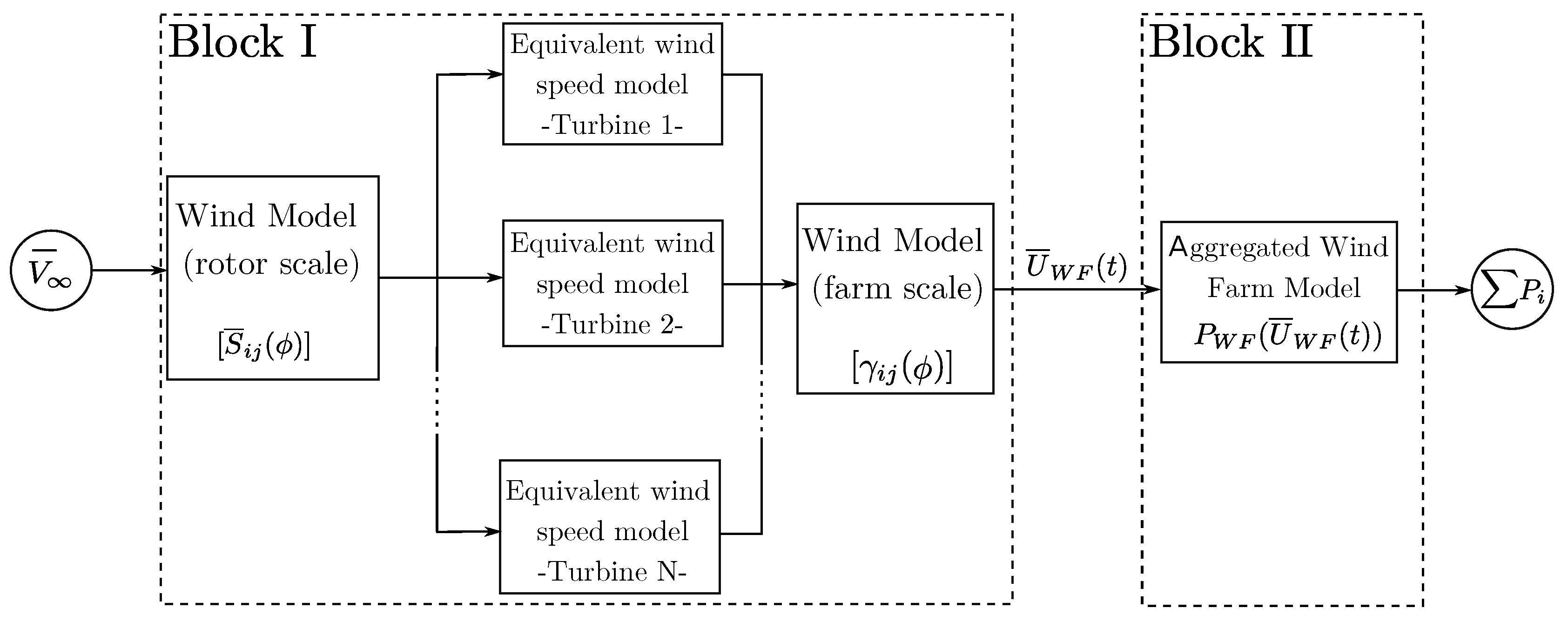
2.2.2. Wind Power Generation


2.3. Demand-Side Model

3. Simulation of Critical Wind Power Fluctuations
- A set of 10,000 2-h series, with a one-second sample rate, of WF wind speed () is firstly estimated. The inputs to the wind farm model are an upstream 2-h average wind speed () according to a Weibull probability distribution, as well as a spectral wind farm model [32,35,40].In this case, the wind is simulated considering a 506-MW offshore wind farm, with 10 rows with 22 wind turbines in each row.
- Realistic wind power data series () are obtained from through an aggregated wind farm power curve [36]. These series correspond to a global period of time of around 2.5 years, which is large enough for obtaining significant wind fluctuations.
- In order to characterize the power oscillations within the series, ramp power rates each of 2-min intervals are calculated (). This interval length is between the characteristic times of frequency control and wind power oscillations.
- Calculated ramp rates () are then sorted in descending order, obtaining the duration curve.
- From the stability point of view, the most critical cases are those where both wind power drops are steep, as well as the wind power share in the current mix of generation is high. Indeed, the ramp rate around the 99th-percentile with the highest wind power share is selected (), and the corresponding 2-h series where this drop happens is identified () within the set of WF power series ().
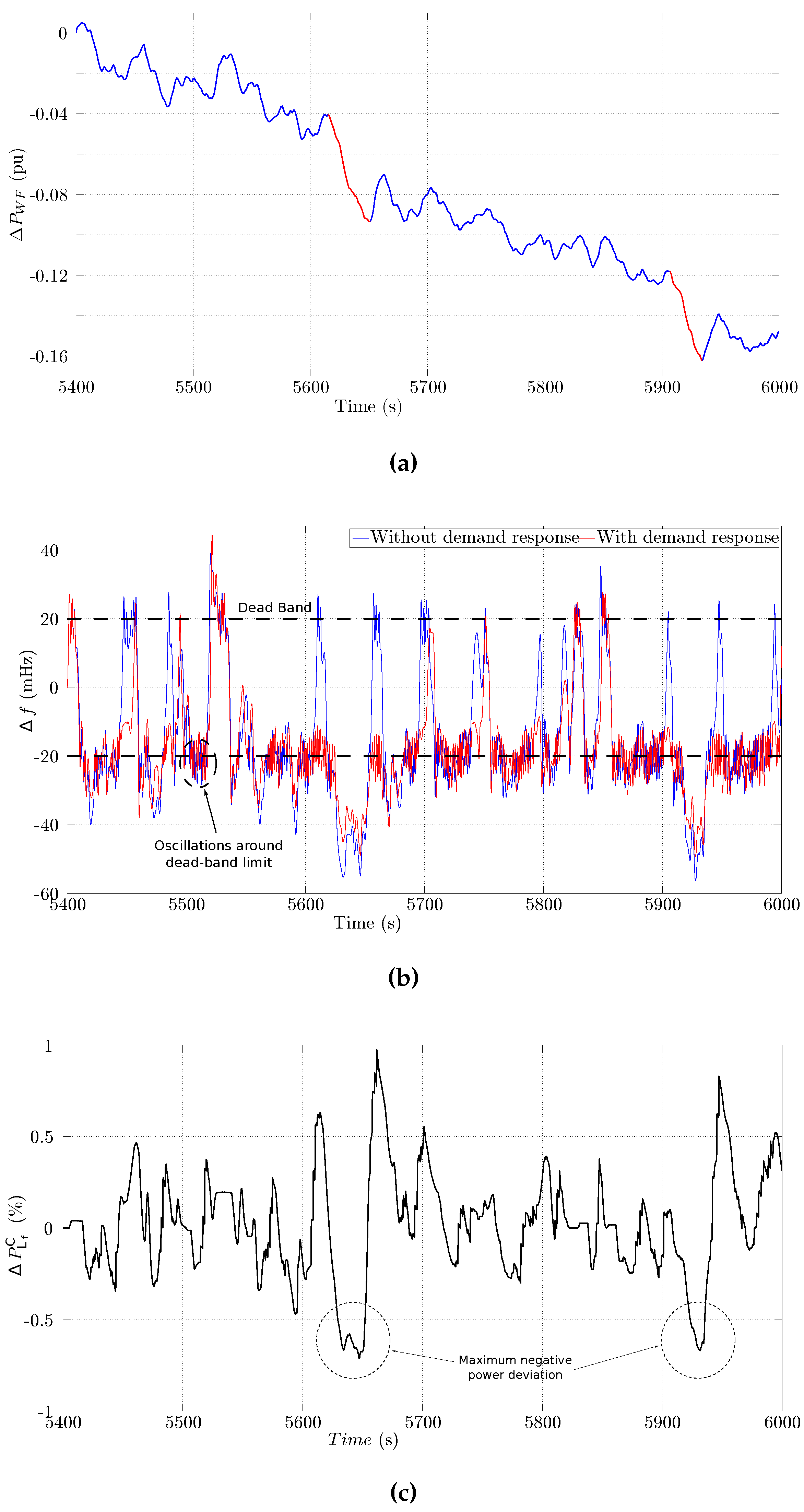
- A 10-min time interval around the event is selected to provide suitable frequency oscillations in the modeled power system . Such a 10-min interval is highlighted in red color in Figure 9.
- Finally, wind power deviation () shown in Figure 2 is determined as the difference between and the expected wind power within this time interval (),


4. Simulation and Results
4.1. Preliminaries

| α | H | ||||||
|---|---|---|---|---|---|---|---|
| 5 % | pu | pu/s | pu/s | pu | 7 s | 0.3 s | 4 s |
4.2. Implemented Scenarios
| Group | Type of load | Share percentage (%) | |
|---|---|---|---|
| Winter | Summer | ||
| I | Refrigeration and freezing | 13.4 | 13.4 |
| II | Space cooling | − | 6.4 |
| II | Space heating | 16.1 | − |
| III | Water heating | 13.5 | 13.5 |
| Total | 43.0 | 33.3 | |
4.3. Analysis of a Case Study: Winter Scenario


| CL (%) | 0 | 2.5 | 5 | 7.5 | 10 |
|---|---|---|---|---|---|
| Winter | - | 5.08 | 9.36 | 16.48 | 19.97 |
| Summer | - | 4.05 | 8.14 | 14.67 | 18.93 |
4.4. Summary of Case Studies


5. Conclusions
Acknowledgments
Author Contributions
Conflicts of Interest
References
- Weisser, D.; Garcia, R.S. Instantaneous wind energy penetration in isolated electricity grids: Concepts and review. Renew. Energy 2005, 30, 1299–1308. [Google Scholar] [CrossRef]
- Doherty, R.; Mullane, A.; Nolan, G.; Burke, D.; Bryson, A.; O’Malley, M. An assessment of the impact of wind generation on system frequency control. IEEE Trans. Power Syst. 2010, 25, 452–460. [Google Scholar] [CrossRef]
- Klempke, H.; McCulloch, C.; Wong, A.; Piekutowski, M.; Negnevitsky, M. Impact of high wind generation penetration on frequency control. In Proceedings of the 20th Australasian Universities Power Engineering Conference (AUPEC), Christchurch, New Zealand, 5–8 December 2010; pp. 1–6.
- Gómez-Expósito, A.; Conejo, A.; Cañizares, C. Electric Energy Systems: Analisys and Operation; CRC Press: Boca Raton, FL, USA, 2009. [Google Scholar]
- Fagan, E.; Grimes, S.; McArdle, J.; Smith, P.; Stronge, M. Grid code provisions for wind generators in Ireland. In Proceedings of the IEEE Power Engineering Society General Meeting, San Francisco, CA, USA, 12–16 June 2005; Volume 2, pp. 1241–1247.
- Mullane, A.; O’Malley, M. The inertial response of induction-machine-based wind turbines. IEEE Trans. Power Syst. 2005, 20, 1496–1503. [Google Scholar] [CrossRef]
- Lalor, G.; Ritchie, J.; Rourke, S.; Flynn, D.; O’Malley, M.J. Dynamic frequency control with increasing wind generation. In Proceedings of the IEEE Power Engineering Society General Meeting, Denver, CO, USA, 6–10 June 2004; pp. 1715–1720.
- Lalor, G.; Mullane, A.; O’Malley, M. Frequency control and wind turbine technologies. IEEE Trans. Power Syst. 2005, 20, 1905–1913. [Google Scholar] [CrossRef]
- Soerensen, P.; Hansen, A.D.; Thomsen, K.; Madsen, H.; Nielsen, H.A.; Poulsen, N.K.; Iov, F.; Blaabjerg, F.; Donovan, M.H. Wind farm controllers with grid support. In Proceedings of the 5th International Workshop on Large-Scale Integration of Wind Power and Transmission Networks for Offshore Wind Farms, Glasgow, UK, 7–8 April 2005.
- Mokadem, M.E.; Courtecuisse, V.; Saudemont, C.; Robyns, B.; Deuse, J. Experimental study of variable speed wind generator contribution to primary frequency control. Renew. Energy 2009, 34, 833–844. [Google Scholar] [CrossRef]
- Morren, J.; de Haan, S.W.H.; Kling, W.L.; Ferreira, J.A. Wind turbines emulating inertia and supporting primary frequency control. IEEE Trans. Power Syst. 2006, 21, 433–434. [Google Scholar] [CrossRef]
- Bousseau, P.; Belhomme, R.; Monnot, E.; Laverdure, N.; Boeda, D.; Roye, D.; Bacha, S. Contribution of wind farms to ancillary services. In Proceedings of the Council on Large Electric Systems (CIGRE) General Meeting, Paris, France, 27 August–1 September 2006.
- Yousefi, A.; Iu, H.C.; Fernando, T.; Trinh, H. An approach for wind power integration using demand side resources. IEEE Trans. Sustain. Energy 2013, 4, 917–924. [Google Scholar] [CrossRef]
- Concordia, C.; Fink, L.; Poullikkas, G. Load shedding on an isolated system. IEEE Trans. Power Syst. 1995, 10, 1467–1472. [Google Scholar] [CrossRef]
- Chuvychin, V.; Gurov, N.; Venkata, S.; Brown, R. An adaptive approach to load shedding and spinning reserve control during underfrequency conditions. IEEE Trans. Power Syst. 1996, 11, 1805–1810. [Google Scholar] [CrossRef]
- Cirio, D.; Demartini, G.; Massucco, S.; Morim, A.; Scalera, P.; Silvestro, F.; Vimercati, G. Load control for improving system security and economics. In Proceedings of the 2003 IEEE Bologna Power Tech Conference Proceedings, Bolgna, Italy, 23–26 June 2003; Volume 4, p. 8.
- Delfino, B.; Massucco, S.; Morini, A.; Scalera, P.; Silvestro, F. Implementation and comparison of different under frequency load–shedding schemes. In Proceedings of the IEEE Power Engineering Society Summer Meeting, Vancouver, BC, Canada, 15–19 July 2001; Volume 1, pp. 307–312.
- Zhao, Q.; Chen, C. Study on a system frequency response model for a large industrial area load shedding. Int. J. Electr. Power Energy Syst. 2005, 27, 233–237. [Google Scholar] [CrossRef]
- Vieira, J.; Freitas, W.; Wilsun, X.; Morelato, A. Efficient coordination of ROCOF and frequency relays for distributed generation protection by using the application region. IEEE Trans. Power Deliv. 2006, 21, 1878–1884. [Google Scholar] [CrossRef]
- Gu, W.; Liu, W.; Zhu, J.; Zhao, B.; Wu, Z.; Luo, Z.; Yu, J. Adaptive decentralized under-frequency load shedding for Islanded smart distribution networks. IEEE Trans. Sustain. Energy 2014, 5, 886–895. [Google Scholar] [CrossRef]
- International Energy Agency. Cool Appliances: Policy Strategies for Energy-Efficient Homes; Organization for Economic Co-operation and Development (OECD): Paris, France, 2003. [Google Scholar]
- Bertoldi, P.; Atanasiu, B. Electricity Consumption and Efficiency Trends in the Enlarged European Union; Technical Report; European Commission – Institute for Environment Sustainability, 2007; Available online: http://ies.jrc.ec.europa.eu (accessed on 9 April 2011).
- Malik, O.; Havel, P. Active demand-side management system to facilitate integration of RES in low-voltage distribution networks. IEEE Trans. Sustain. Energy 2014, 5, 673–681. [Google Scholar] [CrossRef]
- Short, J.A.; Infield, D.G.; Freris, L.L. Stabilization of grid frequency through dynamic demand control. IEEE Trans. Power Syst. 2007, 22, 1284–1293. [Google Scholar] [CrossRef] [Green Version]
- Molina-García, A.; Bouffard, F.; Kirschen, D. Decentralized demand-side contribution to primary frequency control. IEEE Trans. Power Syst. 2011, 26, 411–419. [Google Scholar] [CrossRef]
- Molina-García, A.; Muñoz Benavente, I.; Hansen, A.; Gómez-Lázaro, E. Demand-side contribution to primary frequency control with wind farm auxiliary control. IEEE Trans. Power Syst. 2014, 29, 2391–2399. [Google Scholar] [CrossRef]
- Samarakoon, K.; Ekanayake, J. Demand side primary frequency response support through smart meter control. In Proceedings of the 44th International Universities Power Engineering Conference (UPEC), Glasgow, UK, 1–4 September 2009; pp. 1–5.
- Kundur, P. Power System Stability and Control; McGraw-Hill: New York, NY, USA, 1994. [Google Scholar]
- Ullah, N.R.; Thiringer, T.; Karlsson, D. Temporary primary frequency control support by variable speed wind turbines—Potential and applications. IEEE Trans. Power Syst. 2008, 23, 601–612. [Google Scholar] [CrossRef]
- REE. P.O. 7.1. Servicio Complementario de Regulación Primaria; Technical Report; Red Eléctrica de España: Madrid, Spain, 1998; Available online: http://www.ree.es (accessed on 20 May 2010).
- UCTE. Operation Handbook – ver. 2.5. Technical Report. European Network of Transmission Network: Brussels, Belgium, 2004. Available online: https://www.entsoe.eu/resources/publications/system-operations/operation-handbook/ (accessed on 8 April 2011).
- Vigueras-Rodríguez, A.; Sørensen, P.; Cutululis, N.; Viedma, A.; Donovan, M. Wind model for low frequency power fluctuations in offshore wind farms. Wind Energy 2010, 13, 471–482. [Google Scholar] [CrossRef]
- Sørensen, P.; Hansen, A.D.; Carvalho-Rosas, P.E. Wind models for simulation of power fluctuations from wind farms. J. Wind Eng. Ind. Aerodyn. 2002, 90, 1381–1402. [Google Scholar] [CrossRef]
- Vigueras-Rodríguez, A. Modelling of the Power Fluctuations in Large Offshore Wind Farms. Ph.D. Thesis, Universidad Politécnica de Cartagena, Cartagena, Spain, 2008. [Google Scholar]
- Sørensen, P.; Cutululis, N.; Vigueras-Rodríguez, A.; Madsen, H.; Pinson, P.; Jensen, L.; Hjerrild, J.; Donovan, M. Modelling of power fluctuations from large offshore wind farms. Wind Energy 2008, 11, 29–43. [Google Scholar] [CrossRef]
- Norgaard, P.; Holttinen, H. A multi-turbine power curve approach. In Proceedings of the Nordic Wind Power Conference (NWPC’04), Gothenburg, Sweden, 1–4 March 2004; Volume 1.
- Wan, Y.; Ela, E.; Orwig, K. Development of an equivalent wind plant power curve. Proc. Wind Power 2010, 1–20. [Google Scholar]
- Iain MacLeay, K.H.; Annut, A. Digest of United Kingdom Energy Statistics 2014; National Statistics Publication: London, UK, 2014. [Google Scholar]
- International Energy Agency (IEA). World Energy Outlook 2014; Technical Report; IEA: Paris, France, 2014; Available online: http://dx.doi.org/10.1787/weo-2014-en (accessed on 14 July 2015).
- Vigueras-Rodríguez, A.; Sørensen, P.; Viedma, A.; Donovan, M.H.; Gómez-Lázaro, E. Spectral coherence model for power fluctuations in a wind farm. J. Wind Eng. Ind. Aerodyn. 2012, 102, 14–21. [Google Scholar] [CrossRef]
- Saidur, R.; Masjuki, H.H.; Jamaluddin, M.Y. An application of energy and exergy analysis in residential sector of Malaysia. Energy Policy 2007, 35, 1050–1063. [Google Scholar] [CrossRef]
- Villena-Lapaz, J.; Vigueras-Rodríguez, A.; Gómez-Lázaro, E.; Molina-García, A.; Fuentes-Moreno, J.A. Stability assessment of isolated power systems with high wind power penetration. In Proceedings of the European Wind Energy Asociation Conference (EWEA), Copenhagen, Denmark, 16–19 April 2012.
© 2015 by the authors; licensee MDPI, Basel, Switzerland. This article is an open access article distributed under the terms and conditions of the Creative Commons by Attribution (CC-BY) license (http://creativecommons.org/licenses/by/4.0/).
Share and Cite
Villena, J.; Vigueras-Rodríguez, A.; Gómez-Lázaro, E.; Fuentes-Moreno, J.Á.; Muñoz-Benavente, I.; Molina-García, Á. An Analysis of Decentralized Demand Response as Frequency Control Support under CriticalWind Power Oscillations. Energies 2015, 8, 12881-12897. https://doi.org/10.3390/en81112349
Villena J, Vigueras-Rodríguez A, Gómez-Lázaro E, Fuentes-Moreno JÁ, Muñoz-Benavente I, Molina-García Á. An Analysis of Decentralized Demand Response as Frequency Control Support under CriticalWind Power Oscillations. Energies. 2015; 8(11):12881-12897. https://doi.org/10.3390/en81112349
Chicago/Turabian StyleVillena, Jorge, Antonio Vigueras-Rodríguez, Emilio Gómez-Lázaro, Juan Álvaro Fuentes-Moreno, Irene Muñoz-Benavente, and Ángel Molina-García. 2015. "An Analysis of Decentralized Demand Response as Frequency Control Support under CriticalWind Power Oscillations" Energies 8, no. 11: 12881-12897. https://doi.org/10.3390/en81112349