Comparison between IEEE and CIGRE Thermal Behaviour Standards and Measured Temperature on a 132-kV Overhead Power Line

Abstract

This paper presents the steady and dynamic thermal balances of an overhead power line proposed by CIGRE (Technical Brochure 601, 2014) and IEEE (Std.738, 2012) standards. The estimated temperatures calculated by the standards are compared with the averaged conductor temperature obtained every 8 min during a year. The conductor is a LA 280 Hawk type, used in a 132-kV overhead line. The steady and dynamic state comparison shows that the number of cases with deviations to conductor temperatures higher than 5 ${}^{\circ }$C decreases from around 20% to 15% when the dynamic analysis is used. As some of the most critical variables are magnitude and direction of the wind speed, ambient temperature and solar radiation, their influence on the conductor temperature is studied. Both standards give similar results with slight differences due to the different way to calculate the solar radiation and convection. Considering the wind, both standards provide better results for the estimated conductor temperature as the wind speed increases and the angle with the line is closer to 90${}^{\circ }$. In addition, if the theoretical radiation is replaced by that measured with the pyranometer, the number of samples with deviations higher than 5 ${}^{\circ }$C is reduced from around 15% to 5%.

1. Introduction

Electricity distribution networks are increasingly affected by new operation scenarios that make integration more complex. Some of these factors are electricity market liberalization and the integration of a large number of renewable installations [1]. As a result, line congestions are increasing, resulting in problems for both the distribution company, which is not capable of absorbing all of the energy generated, resulting in a decrease in efficiency, and the generation company because it will be requested to limit production and, in some cases, to stop it. These scenarios produce great inefficiencies in the system from both energy and environmental aspects because the generation of clean energy is limited to avoid problems in the distribution lines.

The basic solution is to increase the distribution and transmission line capacity, which can be performed in several ways. The most obvious way is to build new lines to reinforce the network. However, this solution is constrained by the high costs and legal difficulties of building new lines [2]. Because of the unviability of the first proposal, electrical line operators are focusing on solutions based on the modification of existing lines and an increase in their capacity.

Increasing the capacity of overhead power lines is currently one of the important areas of research due to a good balance between the results obtained and the costs involved. There are different techniques to increase this capacity: determine meteorological conditions by means of deterministic [3] or probabilistic [4] methods, up to the newest innovations in smart grids and line parameters real-time monitoring: temperature, sag, tilt, power, current and weather conditions [5,6,7].

In the case of wind farm integration into the grid, monitoring weather conditions in real time can be very useful to obtain a win-win situation [8,9]. Strong winds increase wind farm production. At the same time, they cool down the conductors of the distribution lines near the farm. This cooling effect allows the grid to be overloaded when it is most needed.

2. Ampacity, Conductor Temperature and Dynamic Calibration of Overhead Lines

The notion of ampacity appeared as a result of research on increasing power line capacity, and it is defined as the maximum amount of electrical current a conductor can continuously carry before sustaining deterioration. Ampacity is limited by several factors: the conductor structure and design, the surrounding environmental conditions and the operating conditions of the line.

Ampacity can be used as a static or dynamic value [10,11,12]. Static ampacity always assumes the most constrained conditions for the conductor and its environment. This condition gives very conservative values and low efficiency grids.

On the other hand, dynamic ampacity considers the variability of the grid and its surroundings (ambient temperature, solar radiation, wind, etc.). Thus, if the different conductor cooling and heating processes are measured in real time, the maximum instantaneous practical current can be measured (dynamic ampacity) without reaching the maximum thermal rating [13,14]. This is why dynamic ampacity is considered to be a more efficient control parameter of the power grid than static ampacity.

Working parameters should be measured or estimated by different methods (deterministic or probabilistic methods) to calculate the ampacity. International Council on Large Electric Systems (in French: Conseil International des Grands Reseaux Electriques, CIGRE) [15] and Institute of Electrical and Electronics Engineers (IEEE) [16] have standards in which the algorithms to estimate the ampacity and the temperature of the conductor are described.

3. Thermal Balance of Overhead Lines Calculation Methods

Both algorithms (CIGRE and IEEE) are based on the thermal balance between the gained and lost heat in the conductor due to the load and environmental conditions [17]. They suggest two ways to estimate the conductor temperature of an overhead power line. The first way uses steady state conditions to calculate the conductor temperature while the second way estimates the temperature in a dynamic balance taking into account the conductor thermal inertia.

The basic thermal balance used in steady state conditions is:

$$q_c+q_r=q_s+q_j+q_m$$

(1)

where $q_c$ is the cooling due to convection, $q_r$ is the cooling due to the radiation to the surroundings, $q_s$ is the heating due to the solar radiation, $q_j$ is the heating due to the Joule effect and $q_m$ is the heating due to the magnetic effect.

If the thermal inertia of the conductor is considered, the following dynamic thermal balance is used instead:

$$mc\frac{d{T}_c}{dt}=q_s+q_j+q_m-q_c-q_r$$

(2)

where m is the mass per unit length, c the specific heat capacity and $T_c$ the theoretical conductor temperature.

The main similarities and differences between both algorithms are [18]:

• Both methods consider the weather conditions, including wind speed and direction, ambient temperature and solar radiation, but they use different approaches to calculate the thermal balance.
• Solar heating is calculated by considering the sun’s position depending on the hour and day of the year. CIGRE uses a more complex algorithm including the direct, diffuse and reflected radiation.
• Convective cooling is approached by CIGRE using Morgan correlations based on Nusselt number and by IEEE using McAdams correlations based on Reynolds number.

Focusing on CIGRE and IEEE standards and in the guide for selection of weather parameters for bare overhead conductor ratings of CIGRE [19], the variables that should be measured or estimated are the ambient temperature ($T_a$), solar radiation ($Q_s$), wind speed ($u_w$), wind direction (${\varphi }_w$) and the current of the conductor ($I_c^{TMS}$). This paper shows the measured conductor surface temperature ($T_c^{TMS}$) and compares it with the temperature estimated by the standards ($T_c^{CIGRE}$ & $T_c^{IEEE}$).

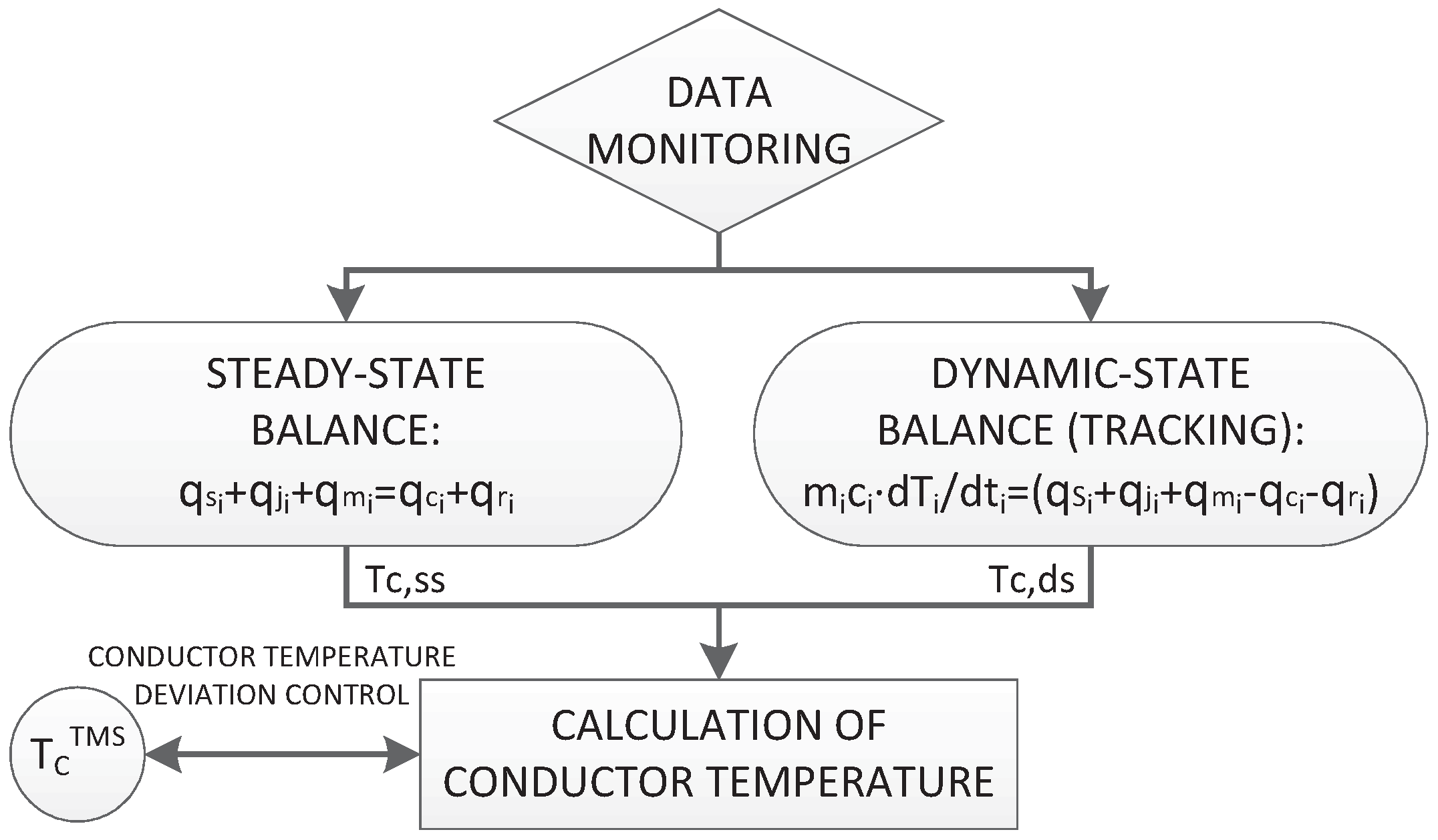
On the one hand, the steady state balance is used and the conductor temperature $T_{c,ss}$ is obtained from the solution of Equation (1). On the other hand, the dynamic state balance is calculated by Equation (2), tracking the conductor temperature $T_{c,ds}$ using a time step $dt$ = 1 s (Figure 1).

Figure 1. Conductor heat balance flow chart.

Figure 1. Conductor heat balance flow chart.

The values of the parameters to calculate the temperature are measured by a meteorological station placed in the tower (ambient temperature, humidity, wind speed and direction and solar radiation). Measured solar radiation is used to compare it with that estimated by the standards and to show the error made by the standards due to the estimated solar radiation use. The conductor temperature calculated for each set of data is then compared with the value measured by a temperature measurement sensor (TMS) placed in the overhead line and close to the meteorological station. This TMS is also used to measure the conductor current needed to calculate $q_j$. All data from meteorological stations and TMS are obtained every second and used to calculate their average values in periods of 8 min.

The evaluation of the optimal place for the location of the weather station has been carried out using both historical data and a meso-scale (convection-permitting) model called HIRLAM (High-Resolution Limited Area Model) that is widely used in Europe for numerical weather prediction. The HIRLAM model had a resolution of 0.05, which means a data grid of 4 km. The resolution of the micro-climatic study was reduced to 500 m by using bi-cubic interpolation. The model also included the surface roughness of the terrain provided by the database CORINE Land Cover. The results provided by the micro-climatic study defined critical points in terms of their ability to cool the cable.

4. Results for a Specific Overhead Line

To study the influence of each variable on the thermal balance of the algorithms, real time data of the ambient and conductor temperature, humidity, wind speed and direction and sun radiation were averaged every 8 min during an entire year—from September 2013 to September 2014— in a 132-kV overhead line with a LA 280 Hawk type conductor [20] located in northern Spain (Figure 2a).

Table 1 describes the variables and the equipment used to measure them. The meteorological station is placed in the electricity tower and the TMS attached to the conductor (Figure 2b).

With the set of values generated, the steady and dynamic thermal states and the associated conductor temperatures according to CIGRE ($T_{c,ss}^{CIGRE}$ and $T_{c,ds}^{CIGRE}$) and IEEE ($T_{c,ss}^{IEEE}$ and $T_{c,ds}^{IEEE}$) are calculated and compared with the conductor temperature measured by the TMS ($T_c^{TMS}$). A large amount of data was processed, and a statistical approach is used to study the individual influence of the variables.

Figure 2. Description of the line and the system components. (a) 132 kV overhead transmission line located in northern Spain; (b) System components of the conductor temperature and meteorological data monitoring at the tower.

Figure 2. Description of the line and the system components. (a) 132 kV overhead transmission line located in northern Spain; (b) System components of the conductor temperature and meteorological data monitoring at the tower.

Table 1. Technical data of the measuring equipment.

Measurement	Measuring Equipment
Conductor Temperature ($T_c^{TMS}$)	TMS Accuracy: 0–120 °C
Conductor current ($I_c^{TMS})$	TMS Accuracy: 100–1500 A
Solar Radiation ($Q_s)$	Pyranometer. Accuracy: 0–1100 $W/m^2$ ±0.5%
Wind Speed ($u_w$)	Vane Anemometer. Accuracy: 0–60 $m/s$ ±0.3 m/s
Wind Angle Relative Direction (${\varphi }_w$)	Vane Anemometer. Accuracy: 0–360°±2°
Ambient Temperature ($T_a$)	Thermometer. Accuracy: (–20)–80 °C ±0.3 °C
Humidity	Hygrometer. Accuracy: 0%–100% ±3%

Table 1. Technical data of the measuring equipment.

Measurement	Measuring Equipment
Conductor Temperature ($T_c^{TMS}$)	TMS Accuracy: 0–120 °C
Conductor current ($I_c^{TMS})$	TMS Accuracy: 100–1500 A
Solar Radiation ($Q_s)$	Pyranometer. Accuracy: 0–1100 $W/m^2$ ±0.5%
Wind Speed ($u_w$)	Vane Anemometer. Accuracy: 0–60 $m/s$ ±0.3 m/s
Wind Angle Relative Direction (${\varphi }_w$)	Vane Anemometer. Accuracy: 0–360°±2°
Ambient Temperature ($T_a$)	Thermometer. Accuracy: (–20)–80 °C ±0.3 °C
Humidity	Hygrometer. Accuracy: 0%–100% ±3%

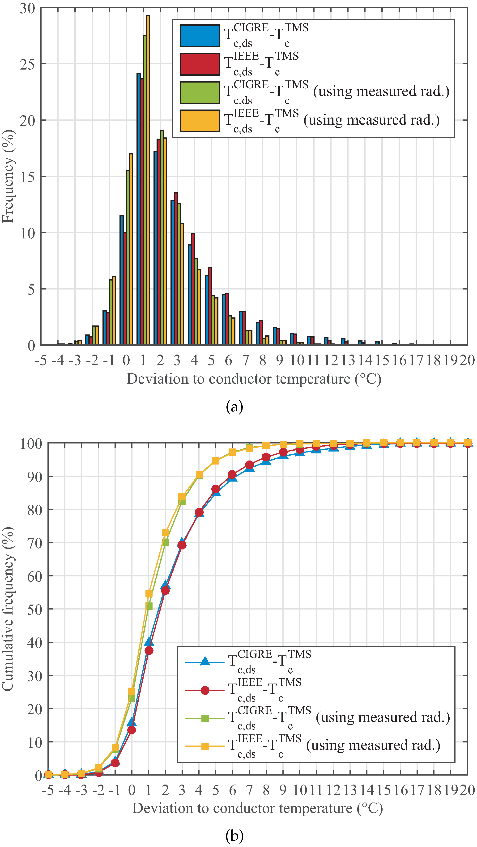
Figure 3a,b and Table 2 provide information regarding the frequency and cumulative frequency of the deviation between the estimated and measured temperatures. Both standards are in good agreement for steady and dynamic balances and underestimate the measured temperature $T_c^{TMS}$ in a 15% of cases.

The steady state assumption does not take into account the thermal inertia of the conductor materials and, thus, it can not model the transition between the set of values. This fact generates peaks in the estimated conductor temperature, which do not, in reality, exist. These mistakes are corrected if the dynamic balance is used, Equation (2). For instance, Table 2 indicates that the number of samples with deviations to conductor temperature lower than 5 ${}^{\circ }$C increases from around 80% to 85% when the dynamic analysis is used.

Table 2. Cumulative frequency of differences between temperatures obtained using CIGRE ($T_{c,ss}^{CIGRE}$ and $T_{c,ds}^{CIGRE}$) and IEEE ($T_{c,ss}^{IEEE}$ and $T_{c,ds}^{IEEE}$) standards and $T_c^{TMS}$ for an entire year.

Deviation	CIGRE S.S.	IEEE S.S.	CIGRE D.S.	IEEE D.S.
Temperature	Cum.Freq.1	Cum.Freq.2	Cum.Freq.3	Cum.Freq.4
(${}^{\circ }$ C)	(%)	(%)	(%)	(%)
–5	0.00	0.00	0.00	0.00
–4	0.01	0.01	0.01	0.00
–3	0.16	0.12	0.14	0.04
–2	0.94	0.87	1.04	0.75
–1	3.93	3.81	4.08	3.68
0	14.77	13.54	15.58	13.70
1	35.34	33.41	39.74	37.37
2	51.05	49.57	56.97	55.67
3	63.37	62.65	69.81	69.20
4	72.89	72.70	78.70	79.14
5	79.62	80.12	84.87	86.02
6	84.51	85.30	89.37	90.59
7	87.76	88.91	92.35	93.56
8	90.22	91.51	94.37	95.76
9	92.38	93.30	95.95	97.24
....	.....	.....	.....	.....
25	99.93	99.96	100.00	100.00

(1)

Steady state cumulative frequency with CIGRE.

(2)

Steady state cumulative frequency with IEEE.

(3)

Dynamic state cumulative frequency with CIGRE.

(4)

Dynamic state cumulative frequency with IEEE.

Table 2. Cumulative frequency of differences between temperatures obtained using CIGRE ($T_{c,ss}^{CIGRE}$ and $T_{c,ds}^{CIGRE}$) and IEEE ($T_{c,ss}^{IEEE}$ and $T_{c,ds}^{IEEE}$) standards and $T_c^{TMS}$ for an entire year.

Deviation	CIGRE S.S.	IEEE S.S.	CIGRE D.S.	IEEE D.S.
Temperature	Cum.Freq.1	Cum.Freq.2	Cum.Freq.3	Cum.Freq.4
(${}^{\circ }$ C)	(%)	(%)	(%)	(%)
–5	0.00	0.00	0.00	0.00
–4	0.01	0.01	0.01	0.00
–3	0.16	0.12	0.14	0.04
–2	0.94	0.87	1.04	0.75
–1	3.93	3.81	4.08	3.68
0	14.77	13.54	15.58	13.70
1	35.34	33.41	39.74	37.37
2	51.05	49.57	56.97	55.67
3	63.37	62.65	69.81	69.20
4	72.89	72.70	78.70	79.14
5	79.62	80.12	84.87	86.02
6	84.51	85.30	89.37	90.59
7	87.76	88.91	92.35	93.56
8	90.22	91.51	94.37	95.76
9	92.38	93.30	95.95	97.24
....	.....	.....	.....	.....
25	99.93	99.96	100.00	100.00

(1)

Steady state cumulative frequency with CIGRE.

(2)

Steady state cumulative frequency with IEEE.

(3)

Dynamic state cumulative frequency with CIGRE.

(4)

Dynamic state cumulative frequency with IEEE.

Figure 3. Frequency and cumulative frequency of differences between temperatures obtained using CIGRE ($T_{c,ss}^{CIGRE}$ and $T_{c,ds}^{CIGRE}$) and IEEE ($T_{c,ss}^{IEEE}$ and $T_{c,ds}^{IEEE}$) standards and the measured conductor temperature ($T_c^{TMS}$) for an entire year. (a) Frequency; (b) Cumulative frequency.

Figure 3. Frequency and cumulative frequency of differences between temperatures obtained using CIGRE ($T_{c,ss}^{CIGRE}$ and $T_{c,ds}^{CIGRE}$) and IEEE ($T_{c,ss}^{IEEE}$ and $T_{c,ds}^{IEEE}$) standards and the measured conductor temperature ($T_c^{TMS}$) for an entire year. (a) Frequency; (b) Cumulative frequency.

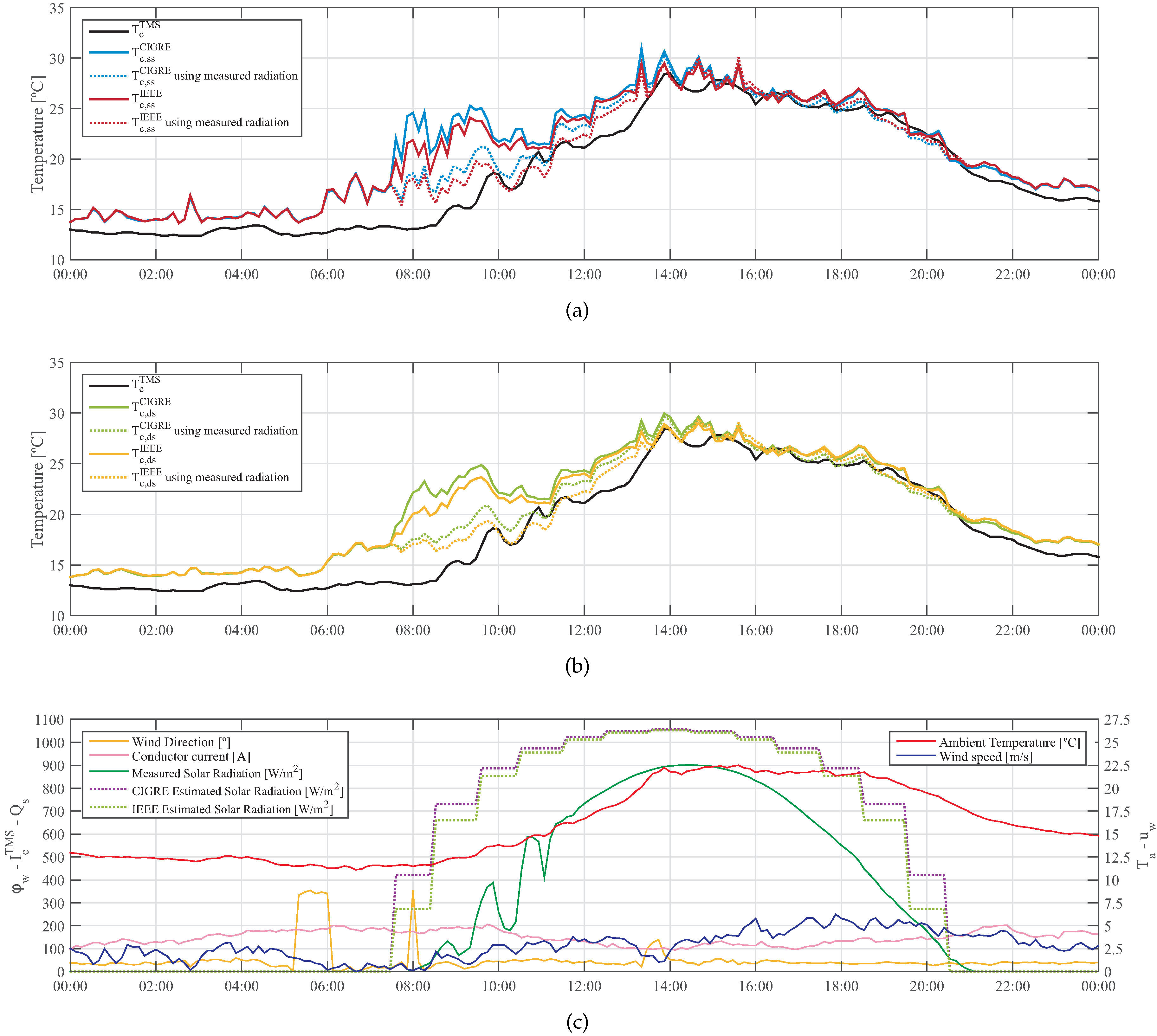
As an example, a representative day (30 August 2014) is shown in Figure 4. Figure 4a shows the deviation between the conductor temperature estimated by CIGRE and IEEE steady state balance ($T_{c,ss}^{CIGRE}$ & $T_{c,ss}^{IEEE}$) and the measured temperature ($T_c^{TMS}$). Figure 4b shows the same deviation for the dynamic state balance. Finally, the measured weather parameters are also represented in Figure 4c.

Comparing Figure 4a,b ,some differences between steady and dynamic balance can be observed. First of all, the dynamic balance models the transient states obtaining smoother curves with less deviations to the conductor temperature giving a better fit than the steady state. Secondly, the consideration of the thermal inertia of the conductor materials makes the slope of the dynamic curves closer to the slope of the $T_c^{TMS}$ curve.

Figure 4. Comparison of conductor temperature obtained using IEEE ($T_{c,ss}^{IEEE}$ and $T_{c,ds}^{IEEE}$) and CIGRE ($T_{c,ss}^{CIGRE}$ and $T_{c,ds}^{CIGRE}$) standards with the measured conductor temperature ($T_c^{TMS}$) for a single day. (a) Steady state balance (30 August 2014); (b) Dynamic state balance (30 August 2014); (c) Weather conditions (30 August 2014).

Figure 4. Comparison of conductor temperature obtained using IEEE ($T_{c,ss}^{IEEE}$ and $T_{c,ds}^{IEEE}$) and CIGRE ($T_{c,ss}^{CIGRE}$ and $T_{c,ds}^{CIGRE}$) standards with the measured conductor temperature ($T_c^{TMS}$) for a single day. (a) Steady state balance (30 August 2014); (b) Dynamic state balance (30 August 2014); (c) Weather conditions (30 August 2014).

From these figures, one can conclude that CIGRE and IEEE estimated temperatures differ more when the influence of radiation is appreciable (from 8:00 to 21:00). These differences between standards are due to the distinct ways to calculate the solar heat gain. CIGRE estimates the direct, diffuse and reflected radiation while IEEE only includes the direct radiation. This is the reason why the CIGRE estimated radiation is higher than the IEEE estimated one, as shown in Figure 4c. This effect makes the CIGRE estimated temperature to be higher than the IEEE estimated one. In addition, a systematic overstimation of the conductor temperature appears in both models when there is no solar radiation (i.e., at night). This deviation, around 2 ${}^{\circ }$C , might be due to the radiative cooling calculation. The equation used to evaluate this effect considers the ground and sky temperature to be equal to the ambient temperature [15,16] but during clear nights this assumption obtains worse estimated conductor temperatures because of radiation to deep space [19].

Figure 4a,b also show the error made if the estimated radiation is used instead of the one measured by the pyranometer. Temperatures obtained using the measured radiation fit better with the conductor temperature $T_c^{TMS}$. Additionally, the frequency and cumulative frequency of the deviation using estimated and measured radiation are plotted in Figure 5. The correction made using the measured radiation is clearly shown. The number of samples with deviations higher than 5 ${}^{\circ }$C decreases from 15% to 5%. However, the number of samples which underestimate the conductor temperature increases 10% (from 15% to 25%). This makes the use of the measured radiation recommendable, but the increase of the underestimated values should also be taken into account.

Figure 5. Frequency and cumulative frequency of differences between temperatures obtained using CIGRE ($T_{c,ds}^{CIGRE}$) and IEEE ($T_{c,ds}^{IEEE}$) standards and $T_c^{TMS}$ for an entire year, with estimated and measured radiation. (a) Frequency; (b) Cumulative frequency.

Figure 5. Frequency and cumulative frequency of differences between temperatures obtained using CIGRE ($T_{c,ds}^{CIGRE}$) and IEEE ($T_{c,ds}^{IEEE}$) standards and $T_c^{TMS}$ for an entire year, with estimated and measured radiation. (a) Frequency; (b) Cumulative frequency.

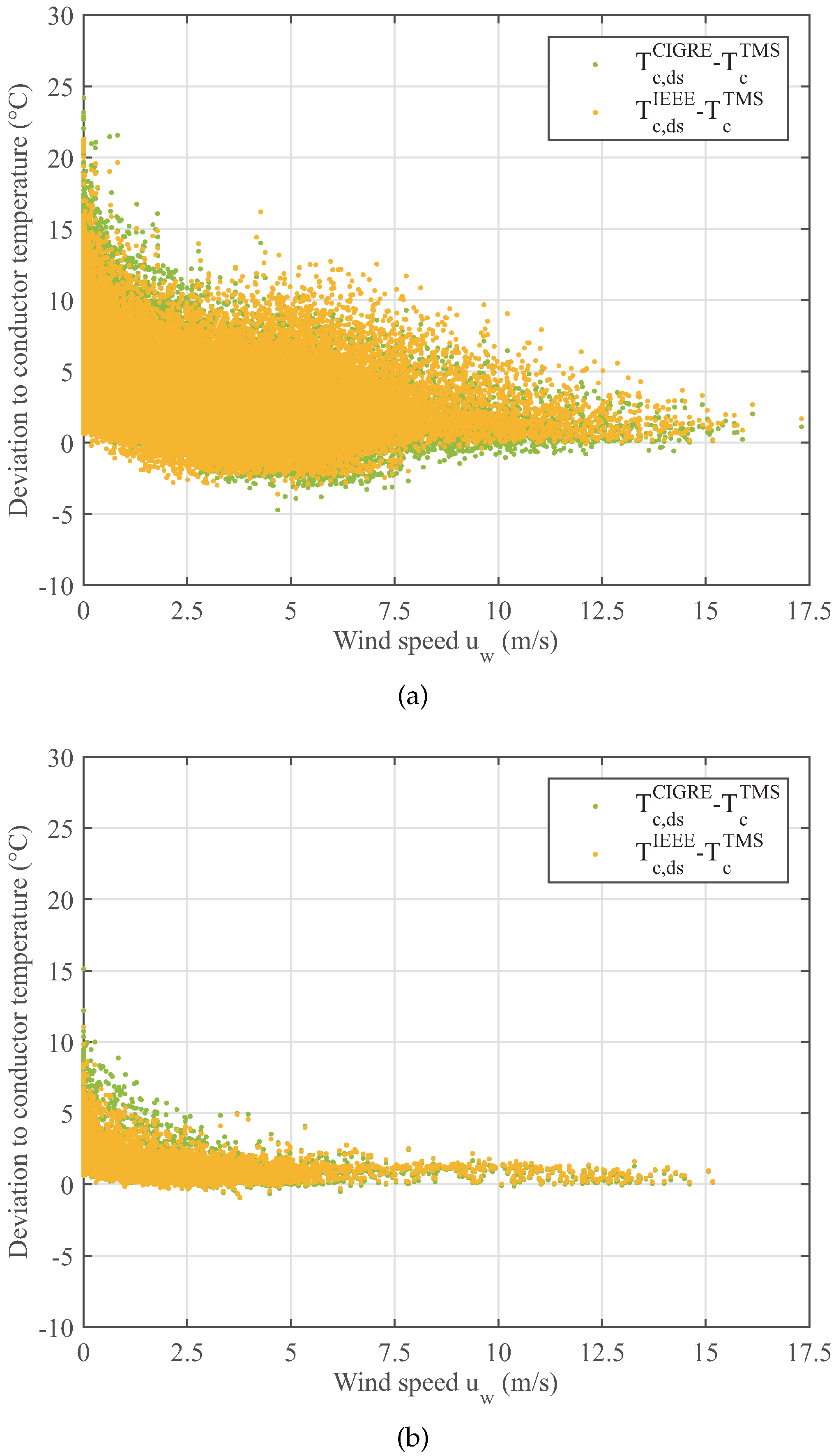
As the dynamic thermal balance provides a better estimated temperature, the dynamic method will be used to study the influence of the wind on the estimated temperature. This influence is reported in previous studies [21] and the wind seems to be the most critical variable for the difference between the estimated and measured temperatures. In Figure 6a, it can be seen that as the wind speed decreases, this difference increases. If the influence of the other variables are minimized by selecting only the cases without solar radiation ($Q_s$ = 0 W/m${}^2$), low radiation losses $q_r$ ($T_c^{TMS}$−$T_a$< 2 ${}^{\circ }$C) and low current ($I_c^{TMS}$< 200 A, the LA-280 maximum current to 80 ${}^{\circ }$C is 600 A), the wind speed influence is clearer, as seen in Figure 6b.

As reported in the standards, the overestimation of the conductor temperature at low speeds is due to the difficulty of having accurate equations to model the convective effect. This fact can make the estimated temperature even 20 ${}^{\circ }$C higher than the measured one.

Figure 6. Deviation of conductor temperature obtained using CIGRE ($T_{c,ds}^{CIGRE}$) and IEEE ($T_{c,ds}^{IEEE}$) standards to the measured conductor temperature ($T_c^{TMS}$) vs. wind speed for an entire year. (a) For all data; (b) $Q_s$ = 0 $W/m^2$, $T_c^{TMS}$−$T_a$< 2°C and $I_c^{TMS}$<200 A.

Figure 6. Deviation of conductor temperature obtained using CIGRE ($T_{c,ds}^{CIGRE}$) and IEEE ($T_{c,ds}^{IEEE}$) standards to the measured conductor temperature ($T_c^{TMS}$) vs. wind speed for an entire year. (a) For all data; (b) $Q_s$ = 0 $W/m^2$, $T_c^{TMS}$−$T_a$< 2°C and $I_c^{TMS}$<200 A.

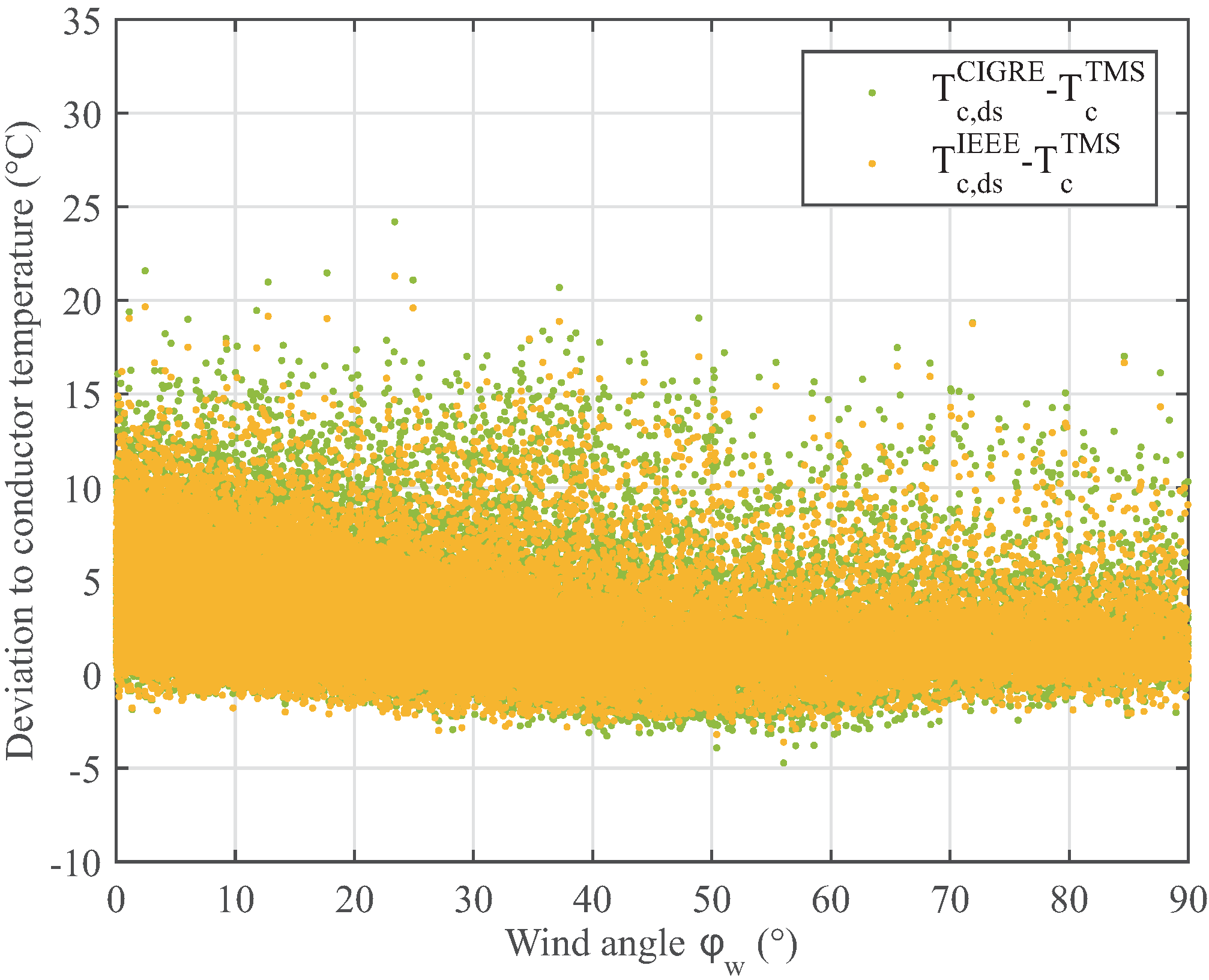
Going deeper into the influence of the wind is to consider how the deviation to conductor temperature is modified by the wind direction. If the temperature deviation is plotted against the angle between the wind and axis of the conductor ${\varphi }_w$ (Figure 7), it can be seen that the lower the wind angle, the higher the deviation is, i.e., in cases with wind blowing parallel to the conductor, standards generally overestimate the conductor temperature.

Finally, Table 3 shows the cumulative frequency of the deviation to conductor temperature lower than 5 ${}^{\circ }$C obtained by the different methods. On the one hand, including the thermal inertia of the conductor materials improves the accuracy of the estimated temperature around 5%. On the other hand, replacing the theoretical radiation by the measured one continues improving the accuracy. In this case, 94.7% of the samples have a deviation lower than 5 ${}^{\circ }$C.

Figure 7. Deviation of conductor temperature obtained using IEEE ($T_{c,ds}^{IEEE}$) and CIGRE ($T_{c,ds}^{CIGRE}$) standards to the measured conductor temperature ($T_c^{TMS}$) vs. the angle between the wind and the axis of the conductor (${\varphi }_w$).

Figure 7. Deviation of conductor temperature obtained using IEEE ($T_{c,ds}^{IEEE}$) and CIGRE ($T_{c,ds}^{CIGRE}$) standards to the measured conductor temperature ($T_c^{TMS}$) vs. the angle between the wind and the axis of the conductor (${\varphi }_w$).

Table 3. Cumulative frequencies of deviation to conductor temperature lower than 5 ${}^{\circ }$C for the studied cases.

Cumulative Frequency	CIGRE S.S.	IEEE S.S.	CIGRE D.S.	IEEE D.S.	CIGRE D.S. (Using Measured Rad.)	IEEE D.S. (Using Measured Rad.)
(%)	79.6	80.1	84.9	86.0	94.7	94.7

Table 3. Cumulative frequencies of deviation to conductor temperature lower than 5 ${}^{\circ }$C for the studied cases.

Cumulative Frequency	CIGRE S.S.	IEEE S.S.	CIGRE D.S.	IEEE D.S.	CIGRE D.S. (Using Measured Rad.)	IEEE D.S. (Using Measured Rad.)
(%)	79.6	80.1	84.9	86.0	94.7	94.7

5. Conclusions

This paper presents the steady and dynamic thermal balances of an overhead power line proposed by CIGRE [15] and IEEE [16] standards. The estimated temperatures calculated by the standards are compared with the averaged conductor temperature obtained every 8 min during an entire year. The conductor is a LA 280 Hawk type, used in a 132-kV overhead line and located in northern Spain.

A good monitoring system of the weather conditions surrounding power lines provides very important information to control the conductor temperature. The evaluation of the optimal place for the location of the weather station has been carried out using both historical data and a meso-scale model. The results provided by the micro-climatic study defined critical points in terms of their ability to cool the cable.

Regarding the type of heat balance, the dynamic method gives a better approach to the conductor temperature. The steady and dynamic state comparison shows that the number of cases with deviations to conductor temperature higher than 5 ${}^{\circ }$C decreases from around 20% to 15% when the dynamic analysis is used (Table 2).

As some of the most critical variables for the IEEE and CIGRE thermal balances are speed and direction of the wind, ambient temperature and solar radiation, their influence on the conductor temperature is studied. Both standards give very similar results with slight differences due to the different way to calculate the solar radiation gain and the convection losses.

CIGRE estimates the direct, diffuse and reflected radiation while IEEE only includes the direct radiation. Focusing on a single day (Figure 4), the estimated temperatures present more differences when the influence of the radiation is appreciable, making the CIGRE estimated temperature to be higher than the IEEE estimated one. Worth noting also is the significant difference between the estimated and the measured temperature if there are large deviations between the estimated and the measured solar radiation (Figure 4c). If the measured radiation on site is used instead of the theoretical one suggested by the standards, the deviation to conductor temperature can also be decreased (Figure 5b). For example, using the estimated radiation, 15% of the samples present deviations higher than 5 ${}^{\circ }$C, while using the measured radiation this percentage decreases to 5%.

Considering the wind, both standards provide better results for the estimated conductor temperature as the wind speed increases (Figure 6a,b) and the angle with the line is closer to 90${}^{\circ }$ (Figure 7), giving the maximum deviation to the measured temperature for low wind speeds and quasi-parallel flows. As reported in the standards, the overestimation of the conductor temperature at low speeds is due to the difficulty of having accurate equations to model the convective effect. This fact can make the estimated temperature to be even 20 ${}^{\circ }$C higher than the measured one.

In conclusion, as the algorithms and the input data are improved, from steady state analysis with estimated radiation to dynamic balance with measured radiation, the accuracy of the estimated temperature can increase up to 15% (Table 3).