
Computational Fluid Dynamics Prediction of a Modified Savonius Wind Turbine with Novel Blade Shapes

Abstract
:1. Introduction
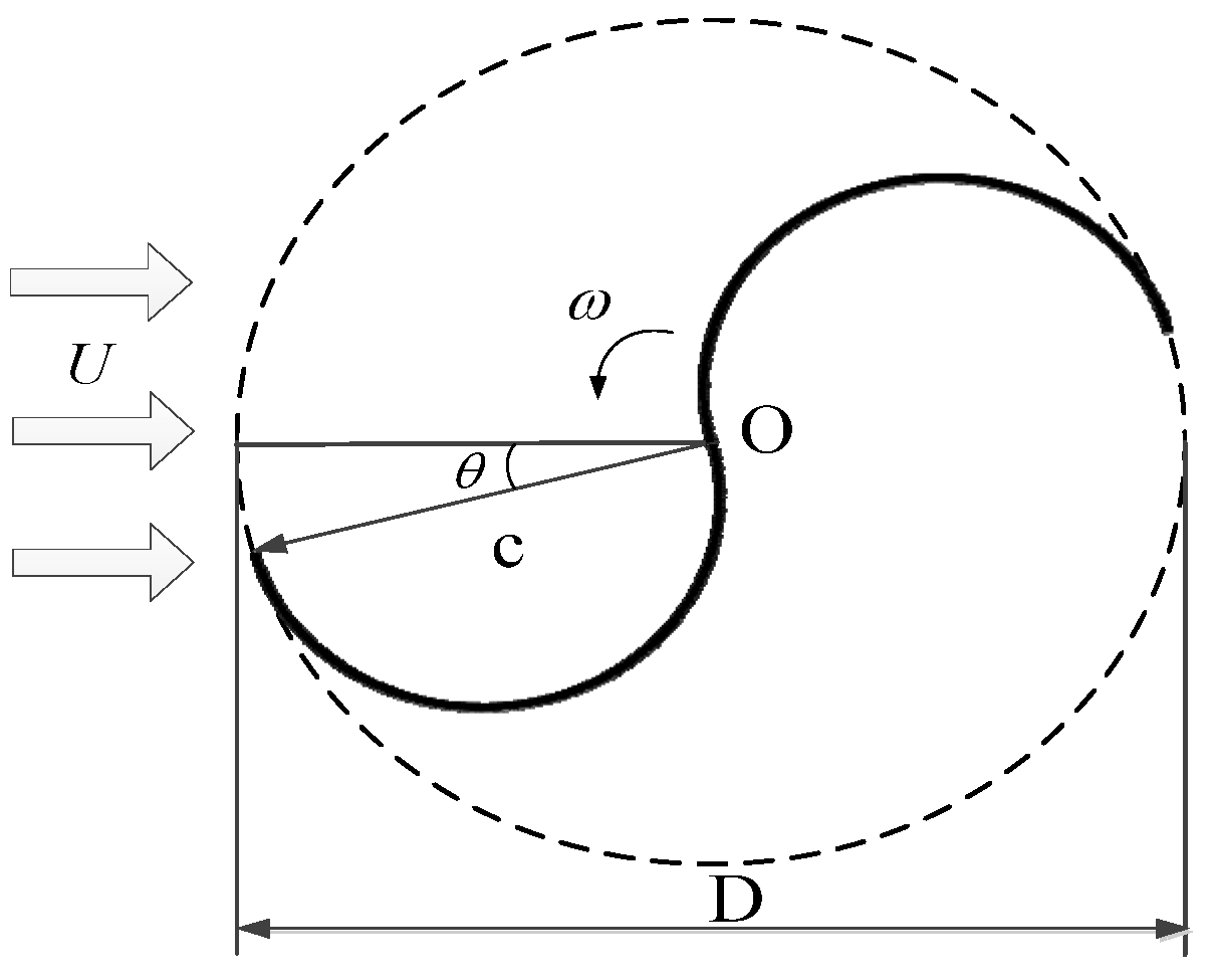
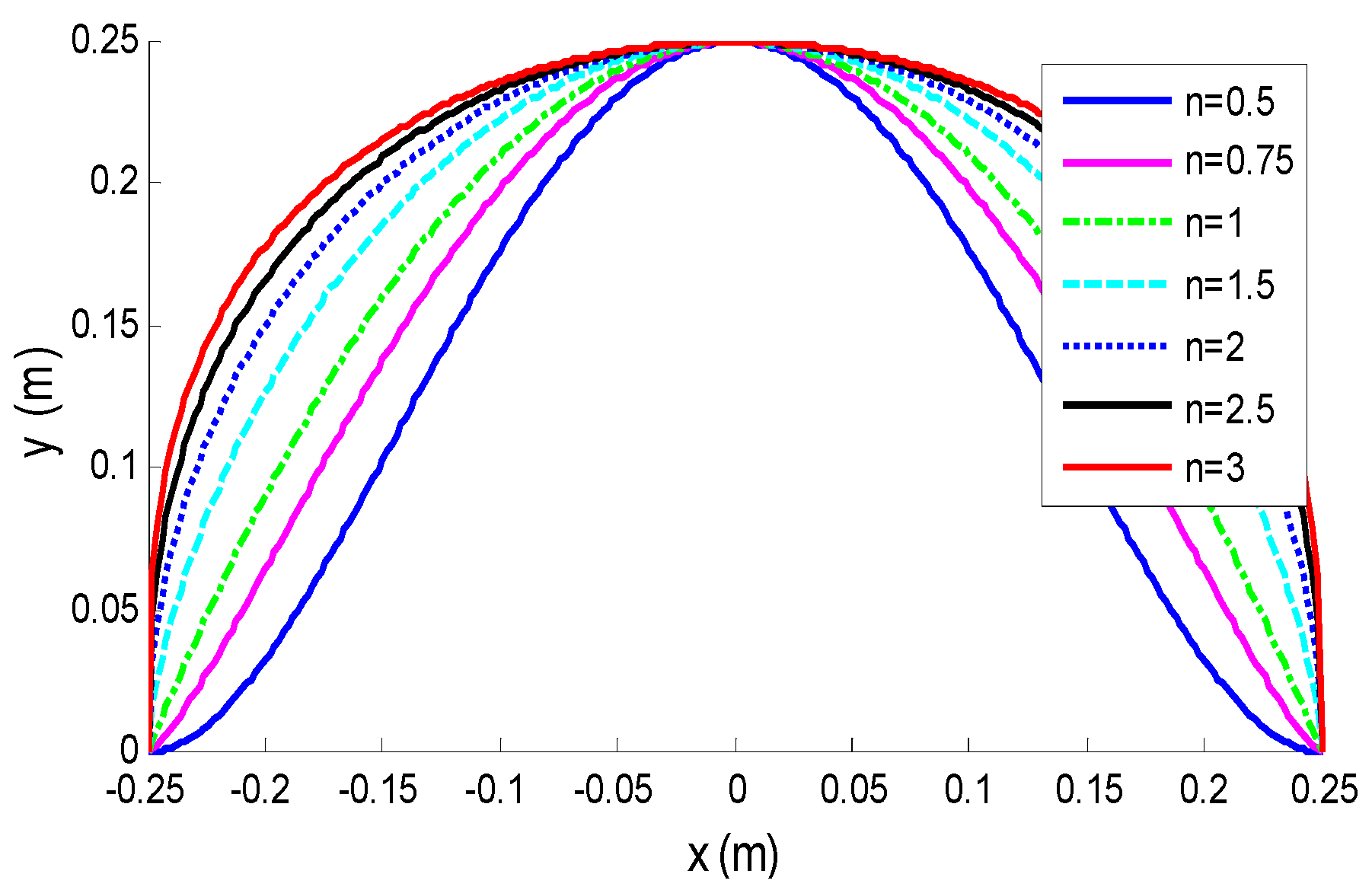
2. The Modified Savonius Wind Turbine and Parameters Definition


| Case | D (m) | C (m) | n |
|---|---|---|---|
| 1 | 1 | 0.5 | 0.5 |
| 2 | 1 | 0.5 | 0.75 |
| 3 | 1 | 0.5 | 1.0 |
| 4 | 1 | 0.5 | 1.5 |
| 5 | 1 | 0.5 | 2.0 |
| 6 | 1 | 0.5 | 2.5 |
| 7 | 1 | 0.5 | 3.0 |
3. Numerical Method
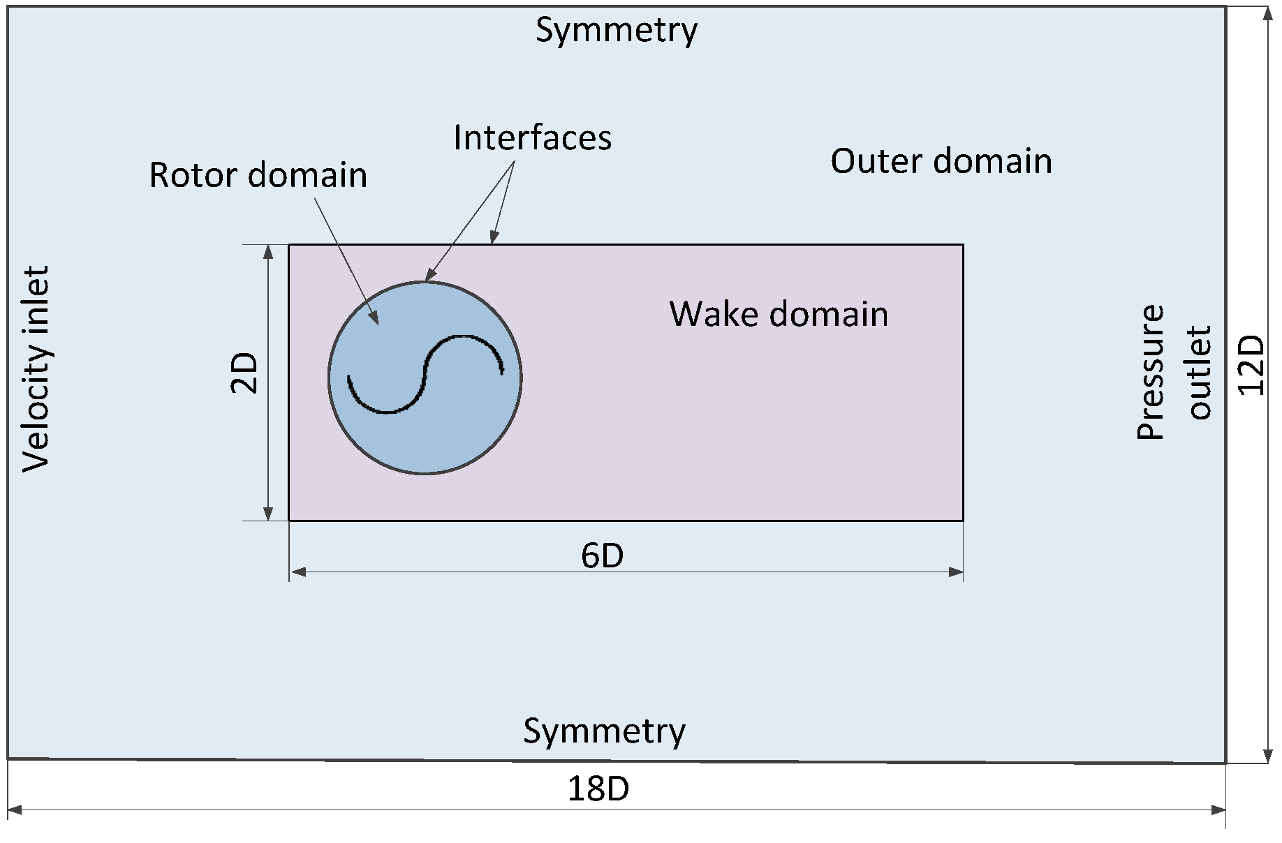
3.1. Computation Domains and Boundary Conditions

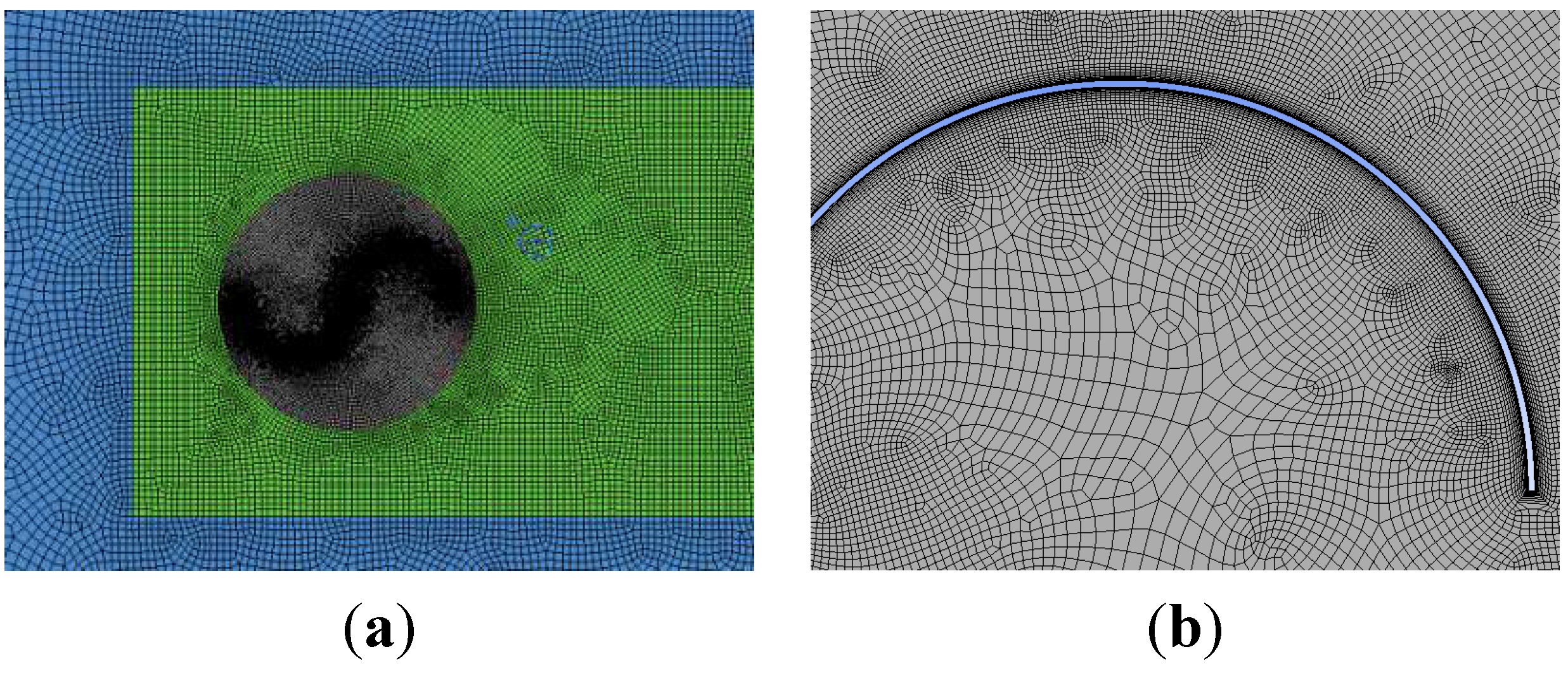
3.2. Grid Generation

3.3. Turbulence Model and Solution Sets
4. Numerical Method Verification and Validation
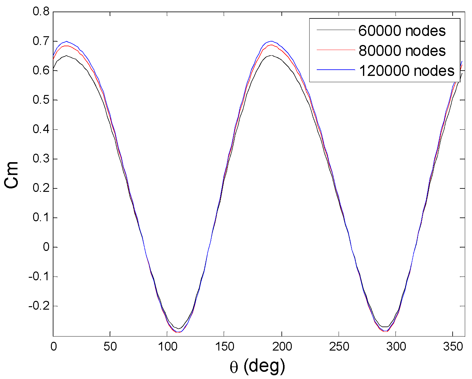
4.1. Verification

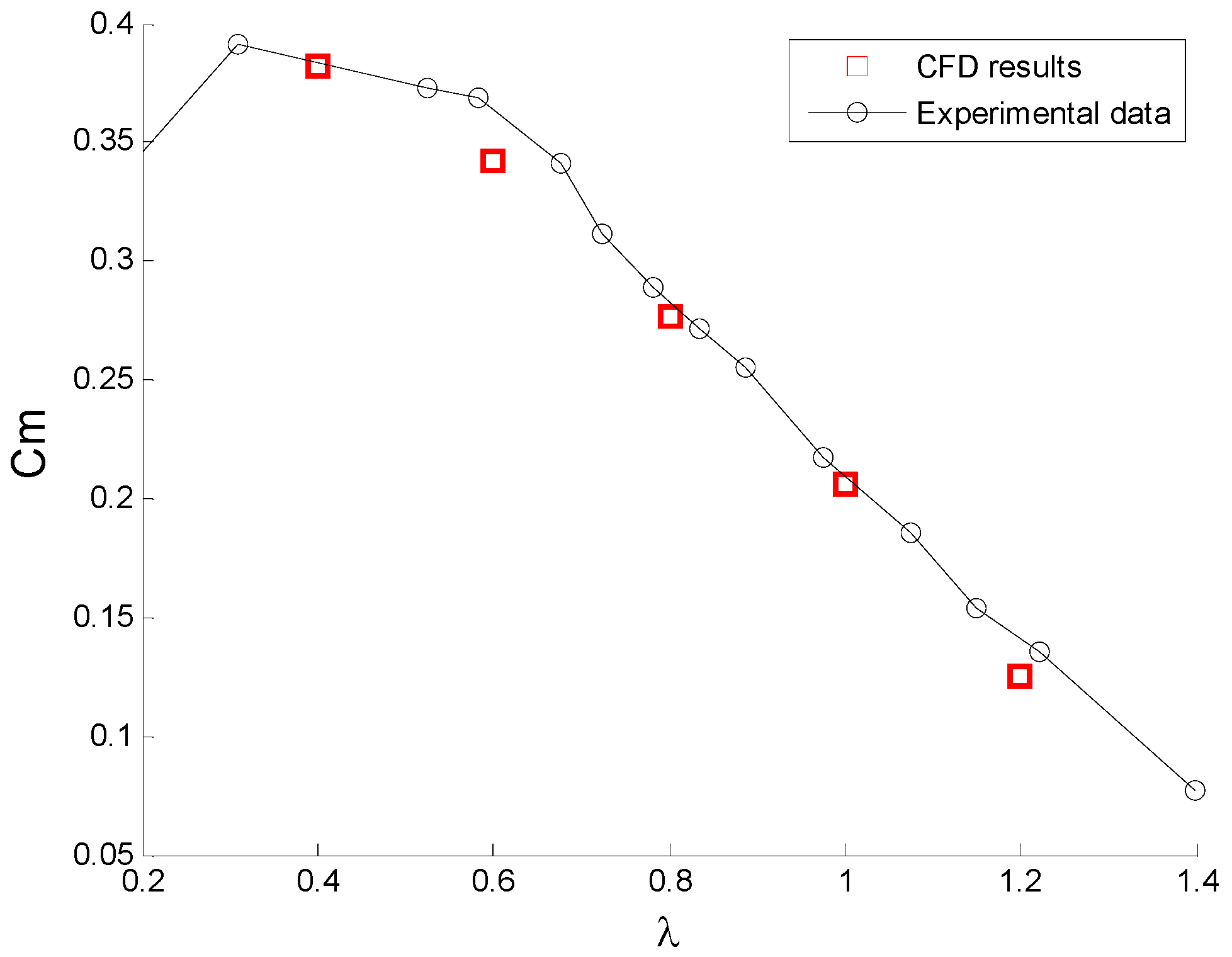
4.2. Validation

5. Results and Discussion
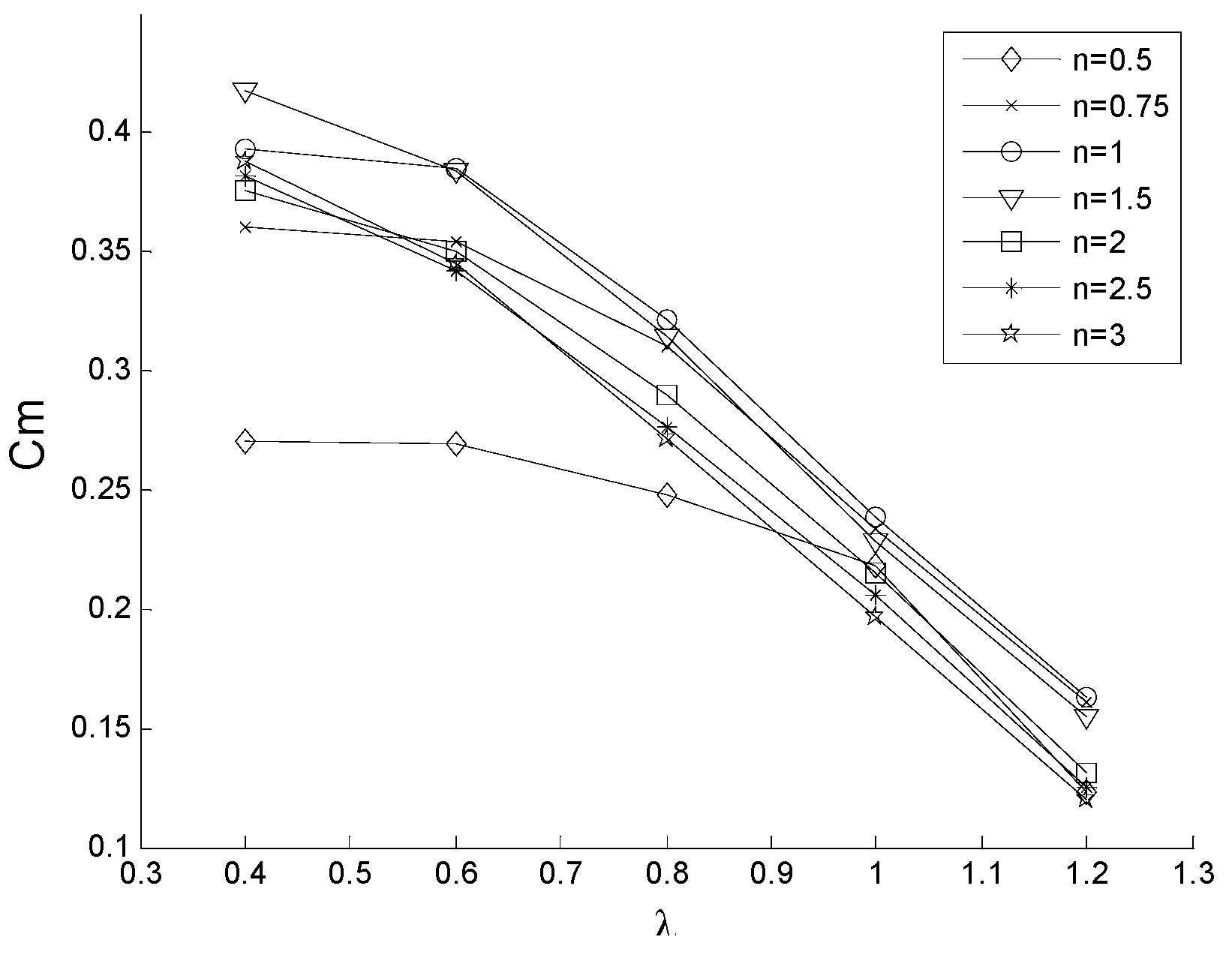
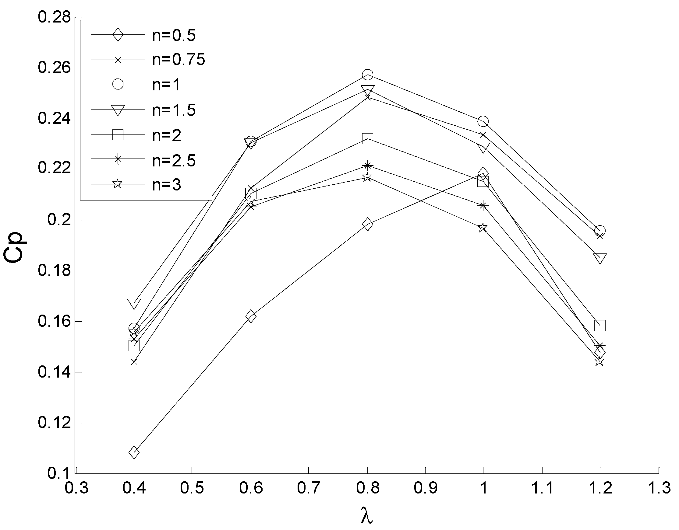
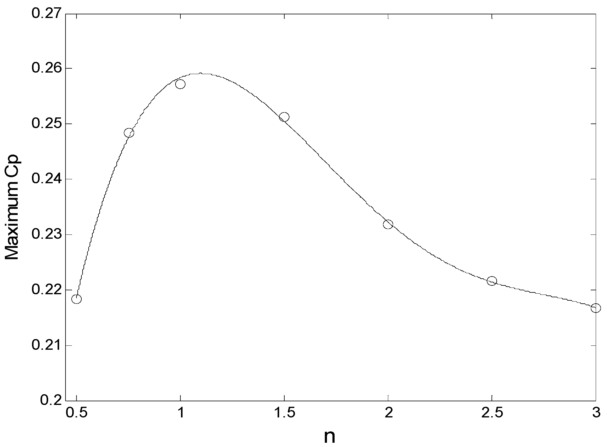
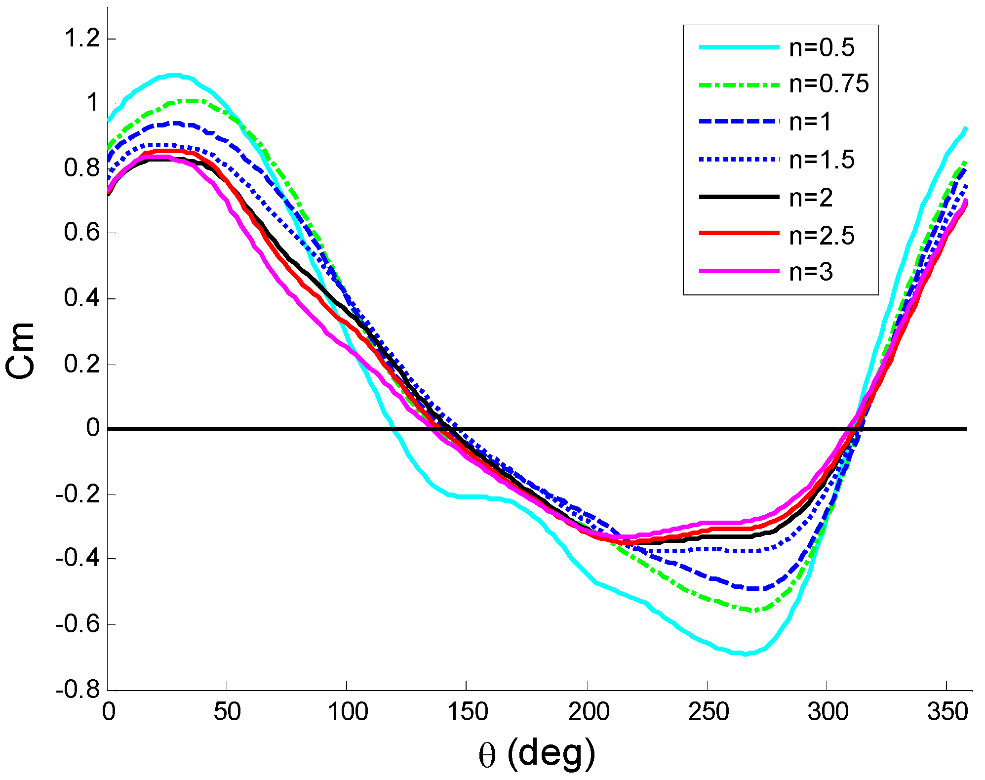
5.1. Torque and Power Characteristics


| Case | n | Peak Cp | Corresponding λ | Cp gain percentage (relative to case 5) |
|---|---|---|---|---|
| 1 | 0.5 | 0.2183 | 1.0 | –5.81 |
| 2 | 0.75 | 0.2482 | 0.8 | 7.14 |
| 3 | 1.0 | 0.2573 | 0.8 | 10.98 |
| 4 | 1.5 | 0.2513 | 0.8 | 8.39 |
| 5 | 2.0 | 0.2318 | 0.8 | 0.00 |
| 6 | 2.5 | 0.2215 | 0.8 | –4.43 |
| 7 | 3.0 | 0.2167 | 0.8 | –6.51 |

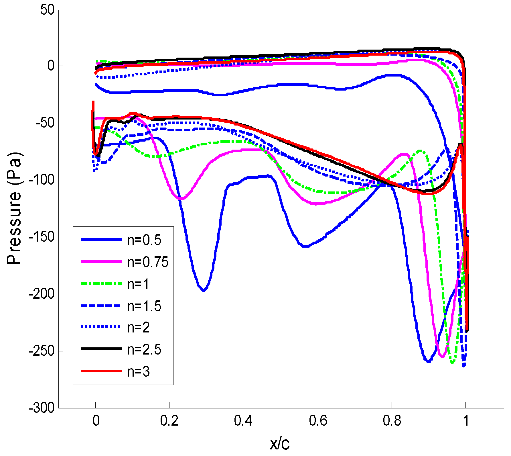
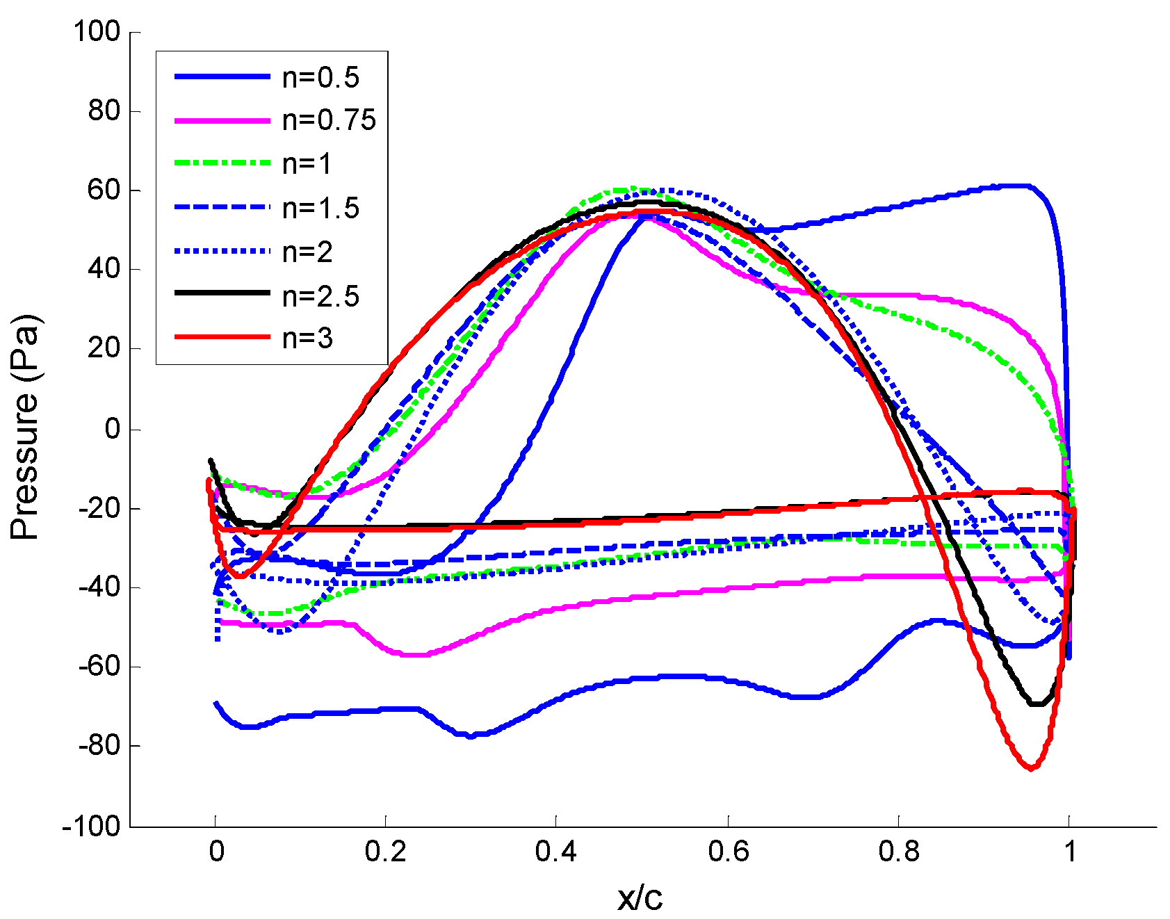
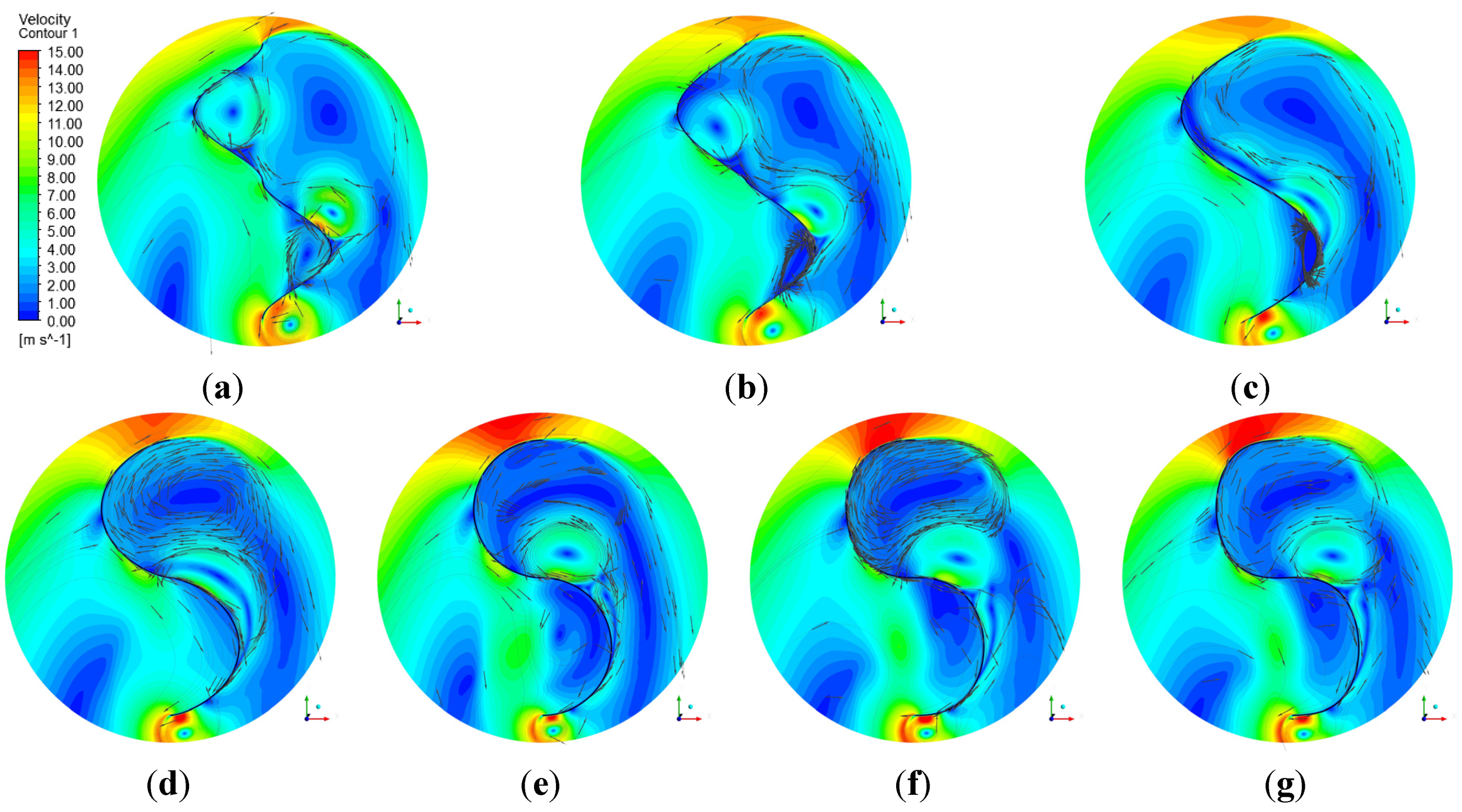
5.2. Mechanism of the Effect of Blade Fullness on the Turbine Performance


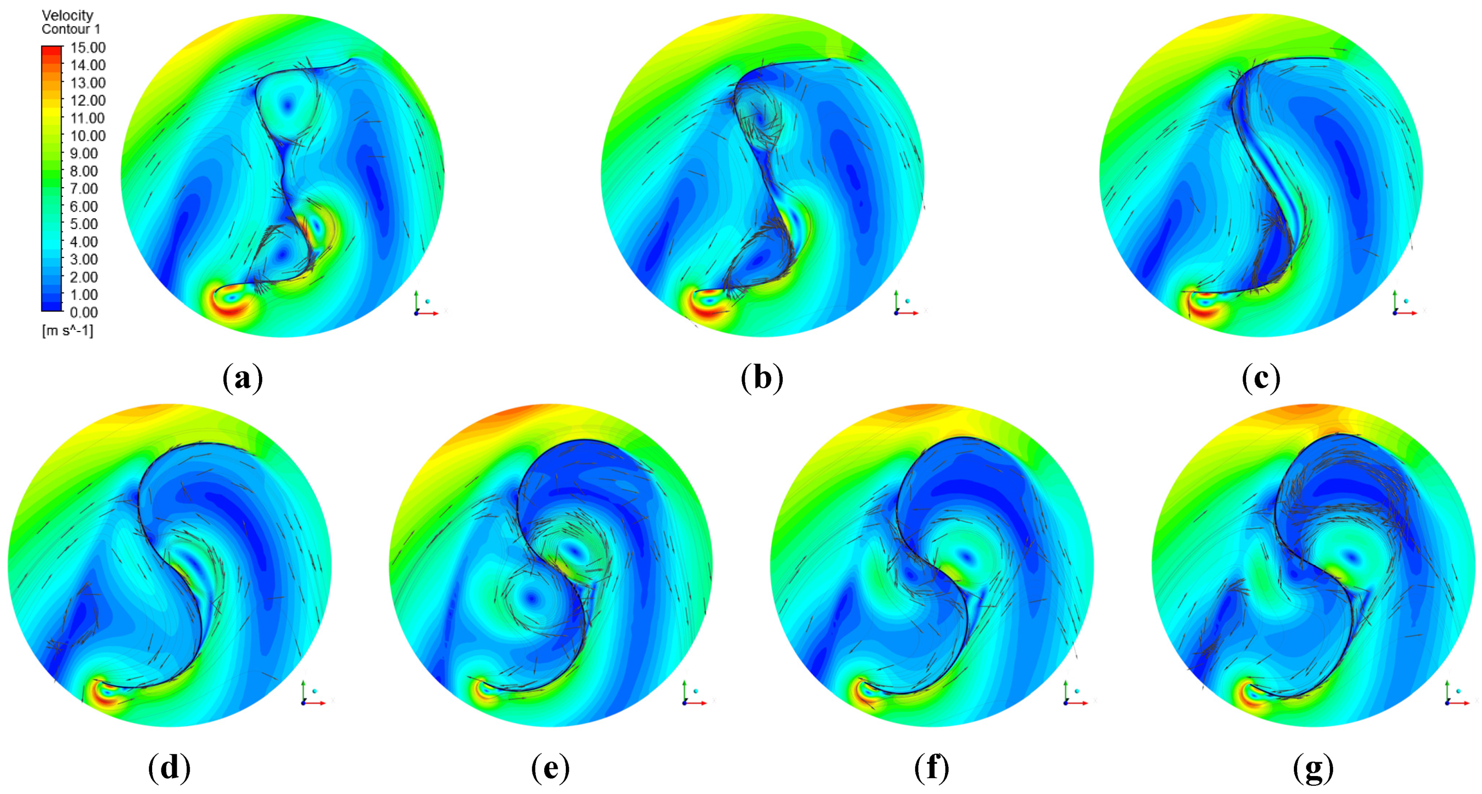
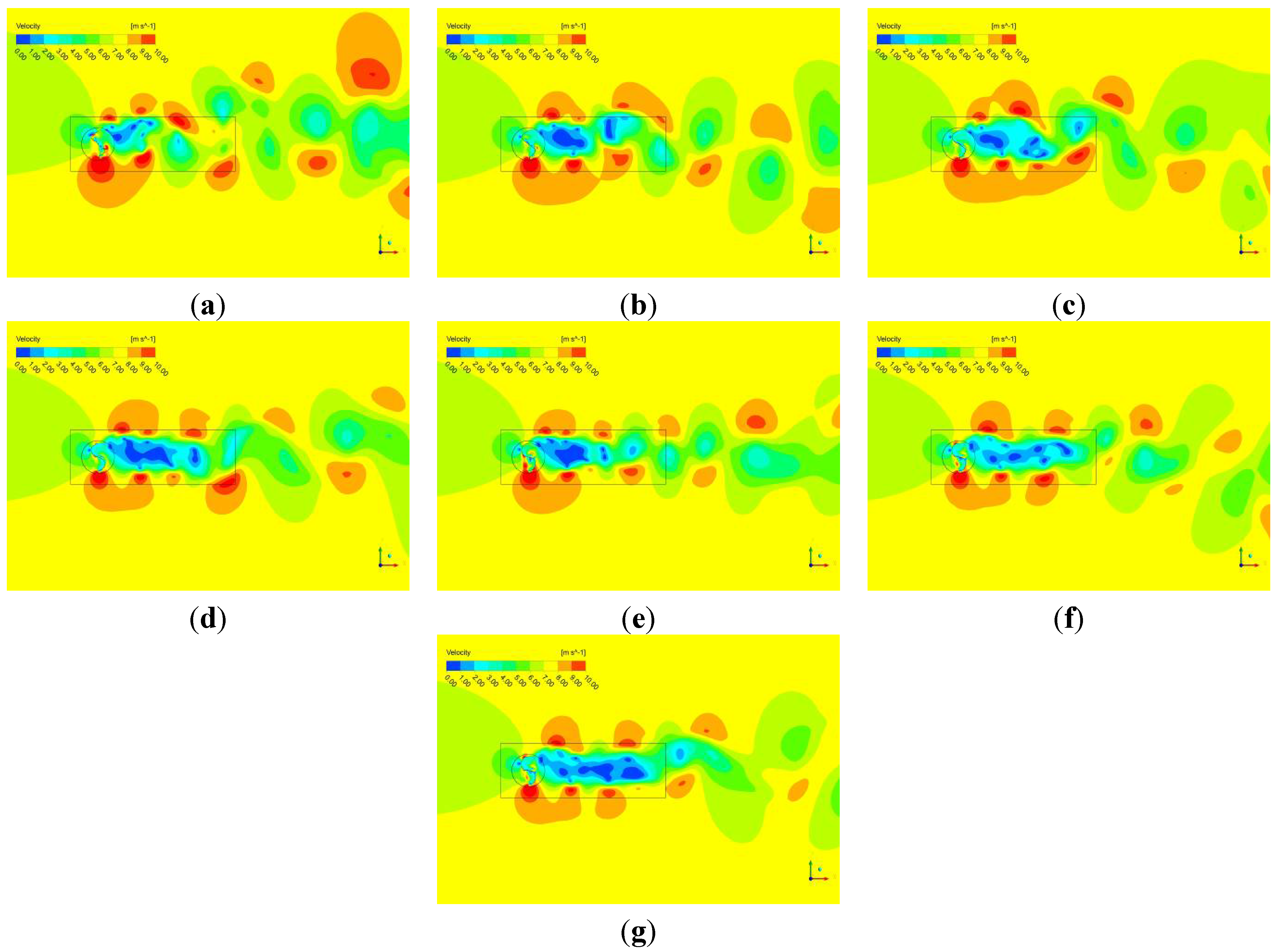
5.3. Effect of the Blade Fullness on Turbine Wake

6. Conclusions
- 1)
- The rotor with a blade fullness of n = 1 has the highest coefficient of power, 0.2573, which is 10.98% higher than a conventional Savonius turbine.
- 2)
- During a rotation period, the blade with a smaller fullness generates both higher positive torque values and lower negative torque values.
- 3)
- Turbines with n ≤ 1 have wider wakes than those of n > 1.
Acknowledgments
Author Contributions
Conflicts of Interest
References
- Yang, B.; Lawn, C. Fluid dynamic performance of a vertical axis turbine for tidal currents. Renew. Energy 2011, 36, 3355–3366. [Google Scholar] [CrossRef]
- Pope, K.; Dincer, I.; Naterer, G. Energy and energy efficiency comparison of horizontal and vertical axis wind turbines. Renew. Energy 2010, 35, 2102–2113. [Google Scholar] [CrossRef]
- Shigetomi, A.; Murai, Y.; Tasaka, Y.; Tasaka, Y. Interactive flow field around two Savonius turbines. Renew. Energy 2011, 36, 536–545. [Google Scholar] [CrossRef]
- Sivasegaram, S. Design parameters affecting the performance of resistance-type, vertical-axis windrotors—An experimental investigation. Wind Energy 1977, 1, 207–217. [Google Scholar]
- Blackwell, B.; Sheldahl, R.; Feltz, L. Wind Tunnel Performance Data for Two-and-Three-Bucket Savonius Rotors; US Sandia Laboratories Report SAND76-0131; Sandia Laboratories: Springfield, VA, USA, 1977. [Google Scholar]
- Rosario, L.; Stefano, M.; Michele, M. 2D CFD modeling of H-Darrieus Wind turbines using a Transition Turbulence Model. Energy Procedia 2014, 45, 131–140. [Google Scholar]
- Saha, U.; Thotla, S.; Maity, D. Optimum design configuration of Savonius rotor through wind tunnel experiments. J. Wind Eng. Ind. Aerodyn. 2008, 96, 1359–1375. [Google Scholar] [CrossRef]
- Hayashi, T.; Li, Y.; Hara, Y. Wind tunnel tests on a different phase three-stage Savonius rotor. JSME Intern. J. 2005, 48, 9–19. [Google Scholar] [CrossRef]
- Akwa, J.; Junior, G.; Petry, A. Discussion on the verification of the overlap ratio influence on performance coefficients of a Savonius wind rotor using computational fluid dynamics. Renew. Energy 2012, 38, 141–149. [Google Scholar] [CrossRef]
- Irabu, K.; Roy, J. Study of direct force measurement and characteristics on blades of Savonius rotor at static state. Exp. Therm. Fluid Sci. 2011, 35, 653–659. [Google Scholar] [CrossRef]
- Kamoji, M.; Kedare, S.; Prabhu, S. Performance tests on helical Savonius rotors. Renew. Energy 2009, 34, 521–529. [Google Scholar] [CrossRef]
- Gupta, R.; Deb, B.; Misra, R. Performance analysis of a helical Savonius rotor with shaft at 45° twist angle using CFD. Mech. Eng. Res. 2013, 3, 118–129. [Google Scholar] [CrossRef]
- Golecha, K.; Eldho, T.; Prabhu, S. Influence of the deflector plate on the performance of modified Savonius water turbine. Appl. Energy 2011, 88, 3207–3217. [Google Scholar] [CrossRef]
- Altan, B.; Atilgan, M. An experimental and numerical study on the improvement of the performance of Savonius wind rotor. Energy Convers. Manag. 2008, 49, 3425–3432. [Google Scholar] [CrossRef]
- Altan, B.; Atilgan, M. An experimental study on improvement of a Savonius rotor performance with curtaining. Exp. Therm. Fluid Sci. 2008, 32, 1673–1678. [Google Scholar] [CrossRef]
- McTavish, S.; Feszty, D.; Sankar, T. Steady and rotating computational fluid dynamics simulations of a novel vertical axis wind turbine for small-scale power generation. Renew. Energy 2012, 41, 171–179. [Google Scholar] [CrossRef]
- Kamoji, M.; Kedare, S.; Prabhu, S. Experimental investigations on single-stage modified Savonius rotor. Appl. Energy 2009, 86, 1064–1073. [Google Scholar] [CrossRef]
- Kacprzak, K.; Liskiewicz, G.; Sobczak, K. Numerical investigation of conventional and modified Savonius wind turbines. Renew. Energy 2013, 60, 578–585. [Google Scholar] [CrossRef]
- Tian, W.; Song, B.; Mao, Z. Numerical investigation of a Savonius wind turbine with elliptical blades. Proc. CSEE 2014, 34, 796–802. [Google Scholar]
- Myring, D.A. Theoretical study of body drag in subcritical axisymmetric flow. Aeronaut. Q. 1976, 27, 186–194. [Google Scholar]
- Fluent 13.0 User’s Guide; ANSYS Inc.: Canonsburg, PA, USA, 2011.
- Sousa, J.V.N.; Macêdo, A.R.L.; Amorim Junior, W.F.; Lima, A.G.B. Numerical analysis of turbulent fluid flow and drag coefficient for optimizing the AUV hull design. Open J. Fluid Dyn. 2014, 4, 263–277. [Google Scholar] [CrossRef]
- Lanzafame, R.; Mauro, S.; Messina, M. Wind turbine CFD modeling using a correlation-based transition model. Renew. Energy 2013, 52, 31–39. [Google Scholar] [CrossRef]
© 2015 by the authors; licensee MDPI, Basel, Switzerland. This article is an open access article distributed under the terms and conditions of the Creative Commons Attribution license (http://creativecommons.org/licenses/by/4.0/).
Share and Cite
Tian, W.; Song, B.; VanZwieten, J.H.; Pyakurel, P. Computational Fluid Dynamics Prediction of a Modified Savonius Wind Turbine with Novel Blade Shapes. Energies 2015, 8, 7915-7929. https://doi.org/10.3390/en8087915
Tian W, Song B, VanZwieten JH, Pyakurel P. Computational Fluid Dynamics Prediction of a Modified Savonius Wind Turbine with Novel Blade Shapes. Energies. 2015; 8(8):7915-7929. https://doi.org/10.3390/en8087915
Chicago/Turabian StyleTian, Wenlong, Baowei Song, James H. VanZwieten, and Parakram Pyakurel. 2015. "Computational Fluid Dynamics Prediction of a Modified Savonius Wind Turbine with Novel Blade Shapes" Energies 8, no. 8: 7915-7929. https://doi.org/10.3390/en8087915
APA StyleTian, W., Song, B., VanZwieten, J. H., & Pyakurel, P. (2015). Computational Fluid Dynamics Prediction of a Modified Savonius Wind Turbine with Novel Blade Shapes. Energies, 8(8), 7915-7929. https://doi.org/10.3390/en8087915