A Mathematical Model and Its Application for Hydro Power Units under Different Operating Conditions

Abstract

This paper presents a mathematical model of hydro power units, especially the governor system model for different operating conditions, based on the basic version of the software TOPSYS. The mathematical model consists of eight turbine equations, one generator equation, and one governor equation, which are solved for ten unknown variables. The generator and governor equations, which are different under various operating conditions, are presented and discussed in detail. All the essential non-linear factors in the governor system (dead-zone, saturation, rate limiting, and backlash) are also considered. Case studies are conducted based on one Swedish hydro power plant (HPP) and three Chinese plants. The simulation and on-site measurements are compared for start-up, no-load operation, normal operation, and load rejection in different control modes (frequency, opening, and power feedback). The main error in each simulation is also discussed in detail. As a result, the model application is proved trustworthy for simulating different physical quantities of the unit (e.g., guide vane opening, active power, rotation speed, and pressures at volute and draft tube). The model has already been applied effectively in consultant analyses and scientific studies.

1. Introduction

Hydro-electricity plays an important role in the safe, stable, and efficient operation of the electric power system. Nowadays, the size of hydro power plants (HPPs) and the structure complexity of the hydraulic-mechanical-electrical system have been increasing. The proportion of electricity generated by intermittent renewable energy sources have also been growing. Therefore, the research on control strategy and transient process of HPPs is of great importance.

Much research has been focused on modeling and dynamic response of hydro turbines [1,2,3,4,5,6], HPPs [7,8,9,10], and pumped storage plants [11,12,13], and many meaningful achievements in hydropower plant models and control [14] have been obtained. Nevertheless, further studies could be improved in the following aspects, which are also the features of this paper: (1) most of the studies mainly focus on single operating conditions. An efficient model and corresponding analysis of various conditions (e.g., start-up, no-load operation, normal operation in different control modes, and load rejection) are needed; (2) the majority of the simulation models are based on MATLAB/Simulink and the form of the mathematical equation set is skipped; the presentation and discussion of mathematical equations under different conditions are meaningful for further development of simulation models.

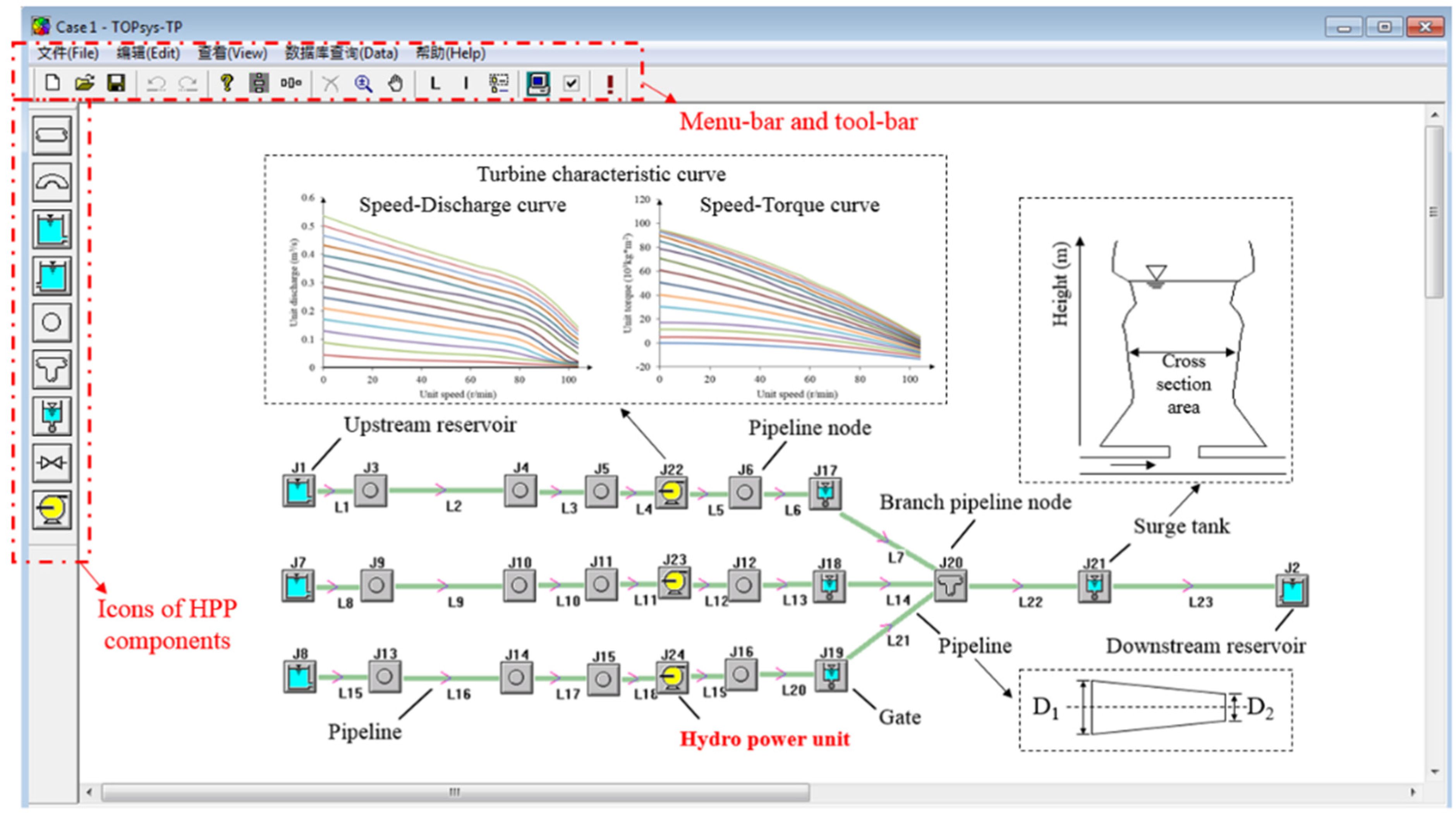
Aiming at these features, this paper presents a mathematical model of hydro power units, especially the governor system model for different operating conditions, based on the existing basic version of software TOPSYS [15,16] by applying Visual C++. The graphical user interface of TOPSYS is shown in Figure 1. Various components of HPPs are represented in different blocks, and the corresponding equations are contained within the blocks. Users could build an HPP model conveniently by dragging and dropping the icons and inputting the parameters. It is worth noting that this study focuses on the model of hydro power units, especially the governor system. Models of other components (e.g., pipeline system) in the HPP system are only shortly presented, more details could be found in [16] and other recent developments are out of the scope of this paper.

In the basic version of TOPSYS, the model of waterway systems and hydraulic turbines has the following characteristics: (1) equations for compressible flow are applied in the draw water tunnel and penstock, considering the elasticity of water and pipe wall; (2) different types of surge tanks and tunnels are included; and (3) characteristic curves of the turbine are utilized, instead of applying simplified transmission coefficients. These characteristics lay a solid foundation for this study to achieve efficient and accurate simulation results.

The remaining content of this paper is organized as follows: Section 2 introduces the mathematical model in detail; Section 3 presents the application of TOPSYS by comparing the simulation and on-site measurement results, based on four engineering cases; Section 4 discusses the overall performance of the model, introduces the related studies of TOPSYS, and suggests future works; and Section 5 condenses the conclusions.

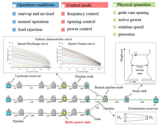
Figure 1. Graphical user interface of TOPSYS and a model of a Swedish hydro power plant (HPP) (Case 1 in Section 3).

Figure 1. Graphical user interface of TOPSYS and a model of a Swedish hydro power plant (HPP) (Case 1 in Section 3).

2. Mathematical Model of Hydro Power Units under Different Operating Conditions

This section presents a mathematical model of hydro power units under different operating conditions, including a model of the turbine governor system improved by this study, and the existing models of other components (pipeline system, turbine, and generator) in the basic version of TOPSYS.

The mathematical hydro power unit model is the core part of the HPP model and the key to describe the hydraulic-mechanical-electrical coupling system. In this study, there are 10 unknown variables in the model of hydro power units: piezo-metric water head (H_p) and discharge at turbine inlet (Q_p), piezo-metric water head (H_s) and discharge at turbine outlet (Q_s), unit rotation speed (n₁₁), unit discharge (Q₁₁), unit moment (M₁₁), mechanical moment of turbine (M_t), resistance moment of generator (M_g) and guide vane opening (y). Therefore the mathematical model consists of 10 equations, more exactly, 8 turbine equations, one generator equation, and 1 governor equation. This section will discuss the generator and governor equations in detail, which are critical to describe different operating conditions of unit.

2.1. Pipeline System

The fundamental equations for the 1-D (one-dimensional) simulation are shown below. Equations of pipeline systems are solved by the characteristic method [17]:

$$\text{Continuity equation}: V\frac{\partial H}{\partial x}+\frac{\partial H}{\partial t}+\frac{a^2}{g}\frac{\partial V}{\partial x}+\frac{a^{2}V}{gA}\frac{\partial A}{\partial x}-\sin \text{θ}\cdot V=0$$

(1)

$$\text{Momentum equation}: g\frac{\partial H}{\partial x}+V\frac{\partial V}{\partial x}+\frac{\partial V}{\partial t}+f\frac{V\left|V\right|}{2D}=0$$

(2)

The details of all the symbols in this paper are given in the Appendix. The pipeline system model in TOPSYS is sophisticated. More exactly, the elastic water hammer effect is considered and different forms of pipelines, channels, and surge tanks are included.

2.2. Turbine

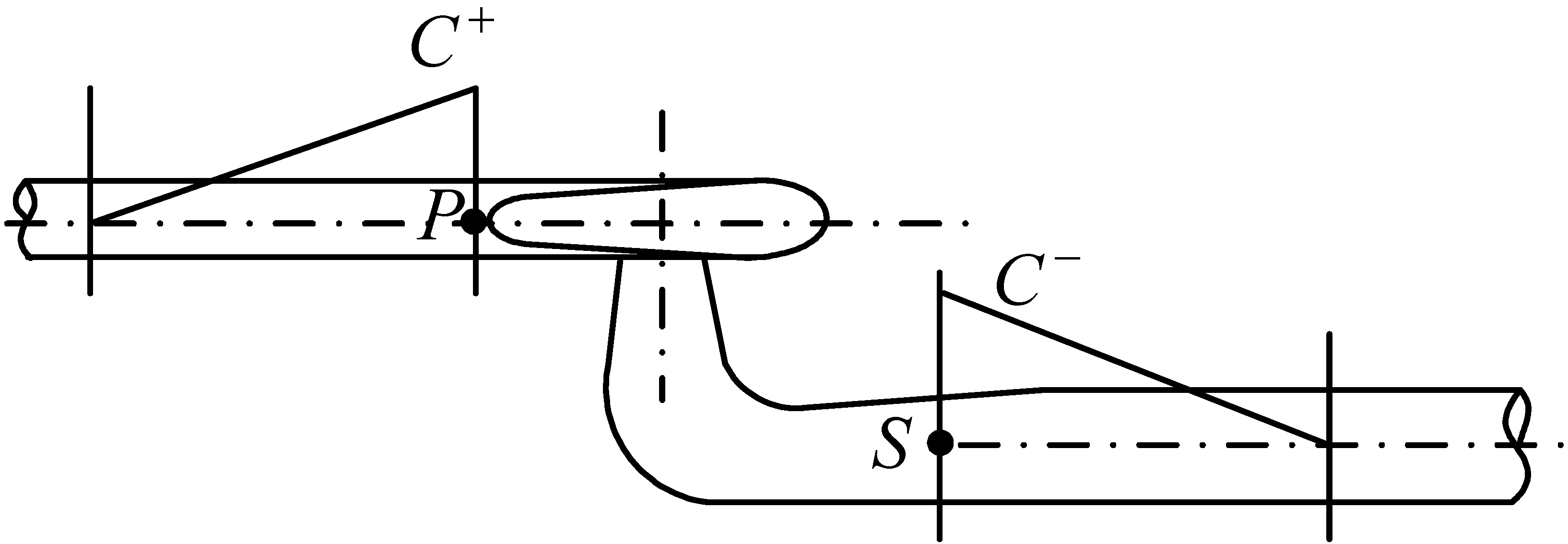
In this paper, the reaction turbine (Francis turbine) is mainly discussed. Table 1 shows the equations of the models and Figure 2 illustrates some of the notation.

Table 1. Equations of the mathematical turbine models.

Description	Equation	Equation number
Continuity equation	$Q_{\text{S}}=Q_{\text{P}}$	(3)
Equations of characteristic method	C+: $Q_{\text{P}}=C_{\text{P}}-B_{\text{P}}{H}_{\text{P}}$	(4)
	C−: $Q_{\text{S}}=C_{\text{M}}+B_{\text{M}}{H}_{\text{S}}$	(5)
Flowing equation of turbine	$Q_{\text{P}}=Q_{11}{D}_1^2\sqrt{\left(H_{\text{P}}-H_{\text{S}}\right)+\Delta H}$	(6)
Equations of unitary parameters	$n_{11}=n{D}_{\text{1}}/\sqrt{\left(H_{\text{P}}-H_{\text{S}}\right)+\mathrm{\Delta }H}$	(7)
	$M_{\text{t}}=M_{11}{D}_1^3\left(H_{\text{P}}-H_{\text{S}}+\mathrm{\Delta }H\right)$	(8)
Characteristic curve equations of turbine	$Q_{11}=f_1\left(n_{11},Y\right)$	(9)
	$M_{11}=f_2\left(n_{11},Y\right)$	(10)

Table 1. Equations of the mathematical turbine models.

Description	Equation	Equation number
Continuity equation	$Q_{\text{S}}=Q_{\text{P}}$	(3)
Equations of characteristic method	C+: $Q_{\text{P}}=C_{\text{P}}-B_{\text{P}}{H}_{\text{P}}$	(4)
	C−: $Q_{\text{S}}=C_{\text{M}}+B_{\text{M}}{H}_{\text{S}}$	(5)
Flowing equation of turbine	$Q_{\text{P}}=Q_{11}{D}_1^2\sqrt{\left(H_{\text{P}}-H_{\text{S}}\right)+\Delta H}$	(6)
Equations of unitary parameters	$n_{11}=n{D}_{\text{1}}/\sqrt{\left(H_{\text{P}}-H_{\text{S}}\right)+\mathrm{\Delta }H}$	(7)
	$M_{\text{t}}=M_{11}{D}_1^3\left(H_{\text{P}}-H_{\text{S}}+\mathrm{\Delta }H\right)$	(8)
Characteristic curve equations of turbine	$Q_{11}=f_1\left(n_{11},Y\right)$	(9)
	$M_{11}=f_2\left(n_{11},Y\right)$	(10)

Figure 2. Illustration of the reaction turbine model.

Figure 2. Illustration of the reaction turbine model.

The coefficients in equations of characteristic method are shown in the Appendix. Functions f₁ and f₂ represent the interpolation of the characteristic curves of the turbine. In this study, for the basic version of TOPSYS, piecewise linear interpolation is applied due to its simplicity and acceptable accuracy for normal cases. A more sophisticated method for the complete characteristic based on space-curved surface [18] is also studied and implemented in advanced versions of TOPSYS.

Equation (11) describes the transform from torque to power output:

$$p_{\text{g}}=M_{\text{t}}\cdot 2\text{π}n/60$$

(11)

2.3. Generator

For generator modeling, the equations are shown in Table 2, and the first-order swing equation is adopted. For the single-machine isolated operation, the equation has the general form, as shown in Equation (12). For the single-machine to infinite bus operation, it is assumed that the rotation speed is constant at the rated value or some other given values, yielding Equation (13). Under off-grid operation, the values of M_g and e_g are 0, and the corresponding Equation (14) can be considered as a special case of Equation (12). The generator frequency, f_g, is transferred from the speed, n.

Table 2. Equations of generator model under different conditions.

Operation condition	Equation	Equation number
Isolated operation (single-machine)	$J\frac{\text{π}}{30}\frac{\text{d}n}{\text{d}t}=M_{\text{t}}-M_{\text{g}}-\frac{30e_{\text{g}}{p}_{\text{r}}}{n_{\text{r}}^2\text{π}}\text{Δ}n$	(12)
Single-machine to infinite bus	$n=n_{\text{c}}(f_{\text{g}}=f_{\text{c}})$	(13)
Off-grid operation	$J\frac{\text{π}}{30}\frac{\text{d}n}{\text{d}t}=M_{\text{t}}$	(14)

Table 2. Equations of generator model under different conditions.

Operation condition	Equation	Equation number
Isolated operation (single-machine)	$J\frac{\text{π}}{30}\frac{\text{d}n}{\text{d}t}=M_{\text{t}}-M_{\text{g}}-\frac{30e_{\text{g}}{p}_{\text{r}}}{n_{\text{r}}^2\text{π}}\text{Δ}n$	(12)
Single-machine to infinite bus	$n=n_{\text{c}}(f_{\text{g}}=f_{\text{c}})$	(13)
Off-grid operation	$J\frac{\text{π}}{30}\frac{\text{d}n}{\text{d}t}=M_{\text{t}}$	(14)

2.4. Governor System

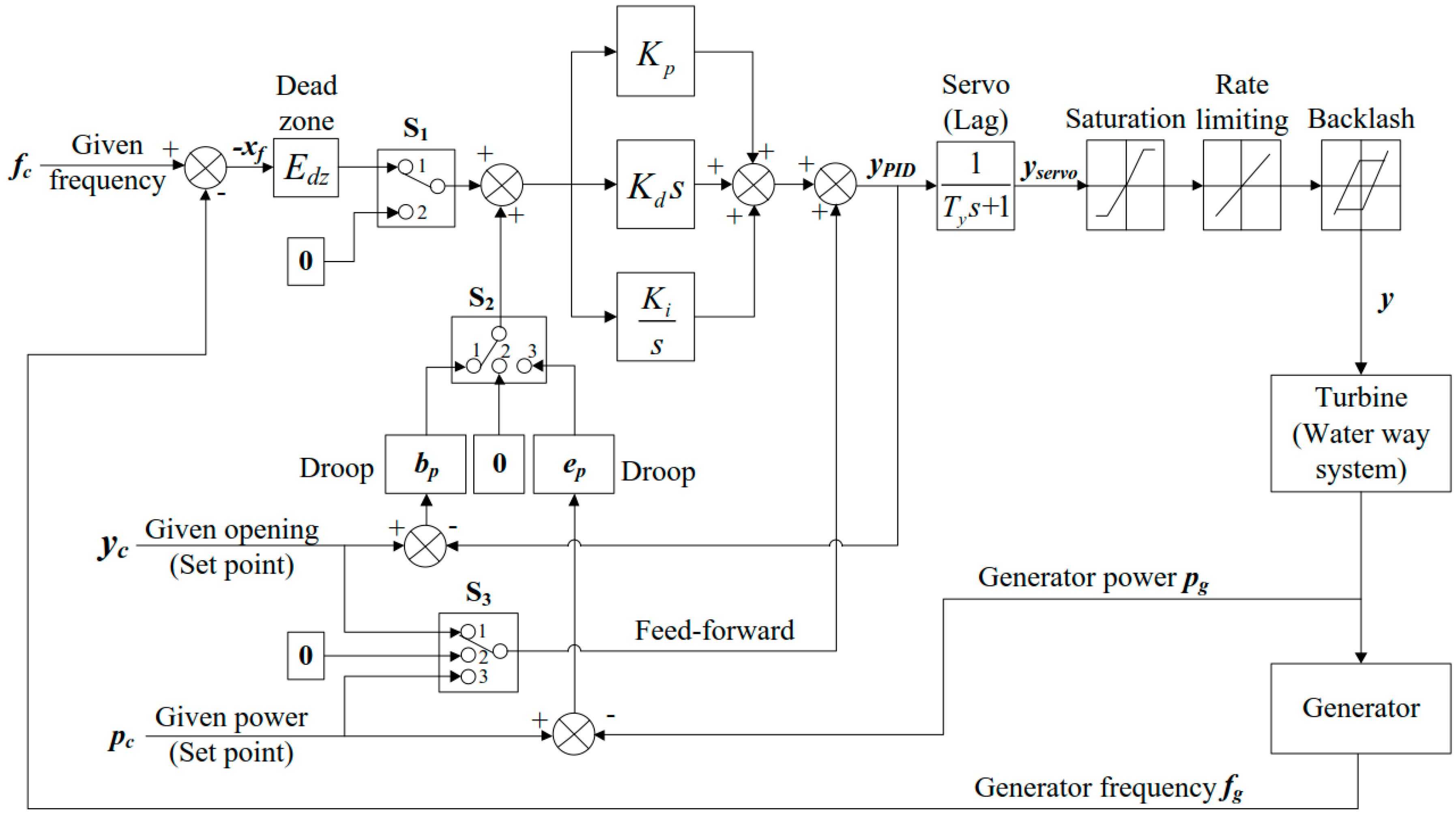
The governor equation has various expressions under different operating conditions and control modes, but the essential objective is the same: to obtain the guide vane opening according to different boundary conditions. Figure 3 demonstrates the complete control block diagram of the proportional-integral-derivative (PID) governor system. Main non-linear factors (dead-zone, saturation, rate limiting, and backlash) are included. All the variables in the governor system are per unit values. The S₁, S₂, and S₃ blocks are selectors between different signals, and the zero input to the selector means no input signal. The number in selectors stands for different statuses, which will be discussed in Section 2.5.

Figure 3. Governor system in TOPSYS.

Figure 3. Governor system in TOPSYS.

2.4.1. Equations for Normal Operation: Load and Frequency Control

Normal operation here stands for isolated and grid-connected operation with load, as shown in Equations (12) and (13), respectively. There are three main control modes: frequency control, opening control, and power control. The main difference between these modes is the input to the control system, i.e., frequency deviation, opening deviation, and power deviation respectively. However, the control signal is the same variable, guide vane opening. This paper establishes a governor model with switchover function of control mode.

(1) Frequency control mode (primary frequency control).

In frequency control mode, as shown in Figure 3, the feedback signal contains not only the frequency value, but also the opening or power, which forms the frequency control under opening feedback and power feedback, as shown in Equations (15) and (16) respectively. They are also two important modes in primary frequency control under grid-connected operation. In isolated operation, if the droop (b_p or e_p) is set to zero, these two modes will be equivalent:

$$b_p{K}_d\frac{d{y_{PID}}^2}{d^{2}t}+(1+b_p{K}_p)\frac{d{y}_{PID}}{dt}+b_p{K}_i(y_{PID}-y_c)=-\left(K_d\frac{d{x_f}^2}{d^{2}t}+K_p\frac{d{x}_f}{dt}+K_i{x}_f\right)$$

(15)

$$e_p{K}_d\frac{d{p_g}^2}{d^{2}t}+e_p{K}_p\frac{d{p}_g}{dt}+e_p{K}_i(p_g-p_c)+\frac{d{y}_{\mathrm{PID}}}{dt}=-\left(K_d\frac{d{x_f}^2}{d^{2}t}+K_p\frac{d{x}_f}{dt}+K_i{x}_f\right)$$

(16)

(2) Opening control mode (secondary frequency control).

In opening control mode, the governor controls the opening according to the given value (y_c). As demonstrated by Figure 3, the opening control is equivalent to the frequency control under opening feedback without frequency deviation input (x_f). Hence, the equation of opening control can be deduced by deleting the frequency (x_f) terms and considering the variable given opening (y_c) and the feed-forward, as shown in Equation (17). Besides, the modeling of the opening control process could be simplified by ignoring the engagement of the PID controller, i.e., setting the opening directly equal to the given value, as shown in Equation (18):

$$b_p{K}_d\frac{d{(y_{\mathrm{PID}}-y_c)}^2}{d^{2}t}+(1+b_p{K}_p)\frac{d(y_{\mathrm{PID}}-y_c)}{dt}+b_p{K}_i(y_{\mathrm{PID}}-y_c)=0$$

(17)

$$y_{\text{PID}}=y_{\text{c}}$$

(18)

(3) Power control mode (secondary frequency control).

In power control mode, the governor controls the opening according to power signals, leading the power output to achieve the given value. As shown by Figure 3, the power control is equivalent to the frequency control under power feedback without frequency deviation input. Hence, the equation of PID power control can be deduced by deleting the frequency (x_f) terms and considering the variable given power (p_c) and feed-forward, as shown in Equation (19). It is worth noting that a simpler controller, without proportional (P) and derivative (D) terms, is applied in many real HPPs, as shown in Equation (20):

$$e_{\text{p}}{K}_{\text{d}}\frac{\text{d}{(p_{\text{g}}-p_{\text{c}})}^2}{{\text{d}}^{2}t}+e_{\text{p}}{K}_{\text{p}}\frac{\text{d}(p_{\text{g}}-p_{\text{c}})}{\text{d}t}+e_{\text{p}}{K}_{\text{i}}(p_{\text{g}}-p_{\text{c}})-\frac{\text{d}{p}_{\text{c}}}{\text{d}t}+\frac{\text{d}{y}_{\text{PID}}}{\text{d}t}=0$$

(19)

$$e_{\text{p}}{K}_{\text{i}}(p_{\text{g}}-p_{\text{c}})-\frac{\text{d}{p}_{\text{c}}}{\text{d}t}+\frac{\text{d}{y}_{\text{PID}}}{\text{d}t}=0$$

(20)

2.4.2. Equations for Start-Up and No-Load Operation

During the start-up process, the hydro power unit is in off-grid operation. Therefore, the generator is represented by Equation (14). There are three start-up modes: open-loop, closed-loop [19], and “open-loop + closed-loop” start-up [20]. Open-loop mode means that the opening control is adopted without the engagement of the PID controller, and Equation (18) is used. In contrast, under the closed-loop mode, the opening is controlled by frequency control, and Equation (15) is applied. However, the given rotation speed (or equivalently generator frequency) is a curve from zero to rated value, instead of a constant rated value. This given curve is obtained usually by testing and tuning. “open-loop + closed-loop” mode is the combination of first two modes: first, the rotation speed increases to a certain set value under open-loop mode; then the controller automatically switches to closed-loop mode to stabilize the speed at the rated value. The set value determining the point of automatic mode switch is usually set to 80% (or larger) of the rated value [20].

The no-load operation mainly refers to the off-grid operation after unit start-up or load rejection, and the generator is modeled by Equation (14). The frequency control, as shown in Equation (15), is applied to stabilize the rotation speed.

2.4.3. Equations for Emergency Stop and Load Rejection

In the testing and analysis of the transient process of an HPP, emergency stops and load rejections [16] are the most dangerous and important conditions, highly concerning the safety of the plant. For both conditions, the resistance moment (M_g) is zero, and the generator is represented by Equation (14). The main differences of modeling for these two conditions are the governor equation and the implementation of closure law of the guide vane emergency stop is governed by Equation (18). The guide vanes are closed by the emergency closing device, and afterwards stay closed. Load rejection, on the other hand, is governed by Equation (15). The process is then under frequency control and the opening increases to no-load opening automatically after the initial closing phase. In the load rejection simulation, the closure speed of guide vane is controlled by the rate limit function.

2.5. Equation Set for Different Operating Conditions

In the governor Equations (15)–(20), only the value of y_PID is solved. For the servo part, the output opening (y_servo) is found by solving:

$$y_{\text{PID}}=T_y\frac{\text{d}{y}_{\text{servo}}}{\text{d}t}+y_{\text{servo}}$$

(21)

Then, the value of final opening (y) is the value after the non-linear functions (dead-zone, saturation, rate limiting, and backlash). The implementation method of non-linear factors in the program can be found in [21].

The selectors (S₁, S₂, and S₃) in the governor system are related to each other. Table 3 shows various status of selectors in different control modes. The status in Figure 3 shows the frequency control under opening feedback, corresponding to Equation (15). Table 4 concludes the equation set, in this study, of hydro power units under different operating conditions.

Table 3. Status of selectors in different control modes.

Control mode	Equation	S1 status	S2 status	S3 status
Frequency control	(15)	1	1	1
	(16)	1	3	3
Opening control	(17)	2	1	1
	(18)	2	2	1
Power control	(19)	2	3	3
	(20)	2	2	3

Table 3. Status of selectors in different control modes.

Control mode	Equation	S1 status	S2 status	S3 status
Frequency control	(15)	1	1	1
	(16)	1	3	3
Opening control	(17)	2	1	1
	(18)	2	2	1
Power control	(19)	2	3	3
	(20)	2	2	3

Table 4. Equation set of the hydro power unit under different operating conditions.

Operating condition		Equation set
		Governor	Generator	Turbine
Normal operation	Frequency control	(15) or (16)	(12) or (13)	(3–10)
	Opening control	(17) or (18)	(12) or (13)
	Power control	(19) or (20)	(12) or (13)
Start-up	Open-loop	(18)	(14)
	Closed-loop	(15)	(14)
No-load operation		(15)	(14)
Emergency stop		(18)	(14)
Load rejection		(15)	(14)

Table 4. Equation set of the hydro power unit under different operating conditions.

Operating condition		Equation set
		Governor	Generator	Turbine
Normal operation	Frequency control	(15) or (16)	(12) or (13)	(3–10)
	Opening control	(17) or (18)	(12) or (13)
	Power control	(19) or (20)	(12) or (13)
Start-up	Open-loop	(18)	(14)
	Closed-loop	(15)	(14)
No-load operation		(15)	(14)
Emergency stop		(18)	(14)
Load rejection		(15)	(14)

3. Model Application: Comparison of Simulation and Measurements

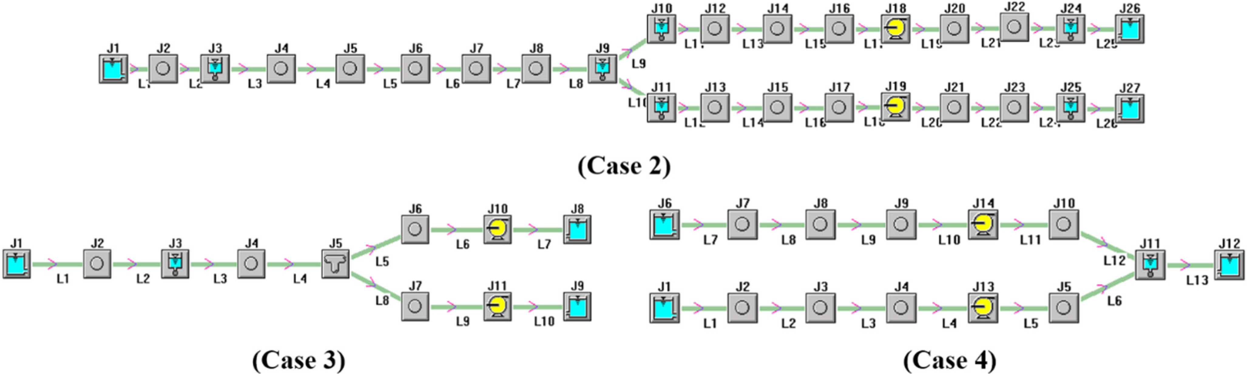
The aim of TOPSYS is to achieve accurate simulation and analysis of different operation cases, e.g., small disturbance, large disturbance, start-up, and no-load operation, etc. This section presents the application of TOPSYS by comparing simulations with on-site measurement results, based on four engineering cases: one Swedish HPP (Case 1 shown in Figure 1) and three Chinese HPPs (Cases 2–4 shown in Figure 4). The details of the cases are shown in

Table A1. Basic information of the engineering cases. Rated values and inertia time constants are for single machines.

Parameter	Case 1	Case 2	Case 3	Case 4
Rated power (MW)	169.2	610.0	51.3	256.5
Rated water head (m)	135.0	288.0	46.0	128.0
Rated discharge (m3/s)	135.0	228.6	122.3	225.0
Rated rotation speed (r/min)	187.5	166.7	136.4	166.7
Inertia time constant Ta (s)	4.98	9.46	9.94	8.75
Surge fluctuation period (s)	390.0	496.0	375	96

in the Appendix. The majority of the measurement data can be directly obtained from the measurement system installed in the HPP.

Figure 4. TOPSYS models of three Chinese HPPs with Francis turbines.

Figure 4. TOPSYS models of three Chinese HPPs with Francis turbines.

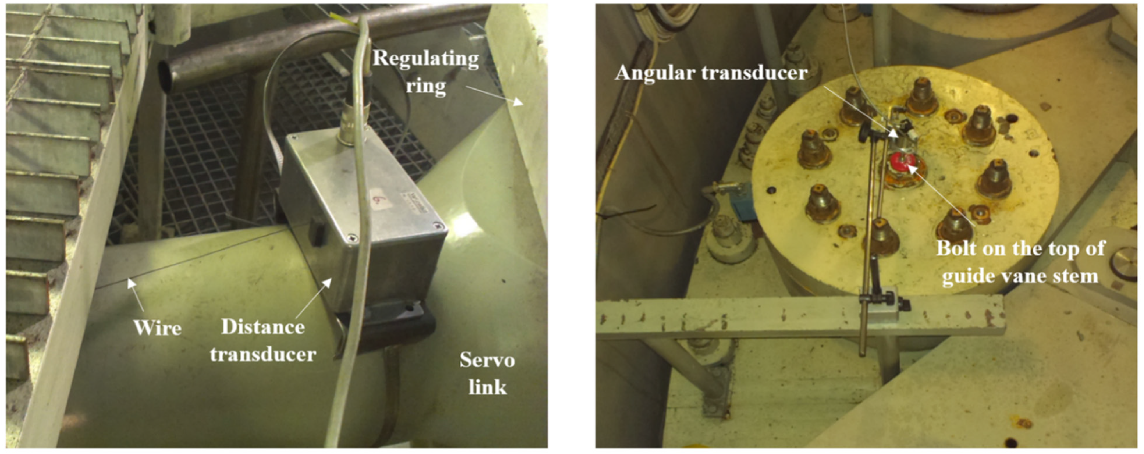
Additional measurements were also conducted, and part of the measurement device is illustrated in Figure 5. All the simulation settings (control mode, governor parameters, etc.) are the same as actual settings and values. All the turbines in these HPP cases are Francis turbines, and other details are found in the Appendix.

Figure 5. Part of measurements for this paper: measuring device for turbine actuator movement. The left figure shows the distance transducer of wire type, which measures position of servo link; the right figure demonstrates the angular transducer which measures guide vane opening.

Figure 5. Part of measurements for this paper: measuring device for turbine actuator movement. The left figure shows the distance transducer of wire type, which measures position of servo link; the right figure demonstrates the angular transducer which measures guide vane opening.

3.1. Small Disturbance: Frequency Control and Load Regulation

3.1.1. Grid-Connected Operation: Primary Frequency Control

For operation under primary frequency control, a fast and stable power response is of great importance. Therefore, an accurate simulation is necessary to test the quality of the power response under different conditions. Figure 6 and Figure 7 show the power response under sinusoidal frequency (Case 1) and frequency step change (Case 2).

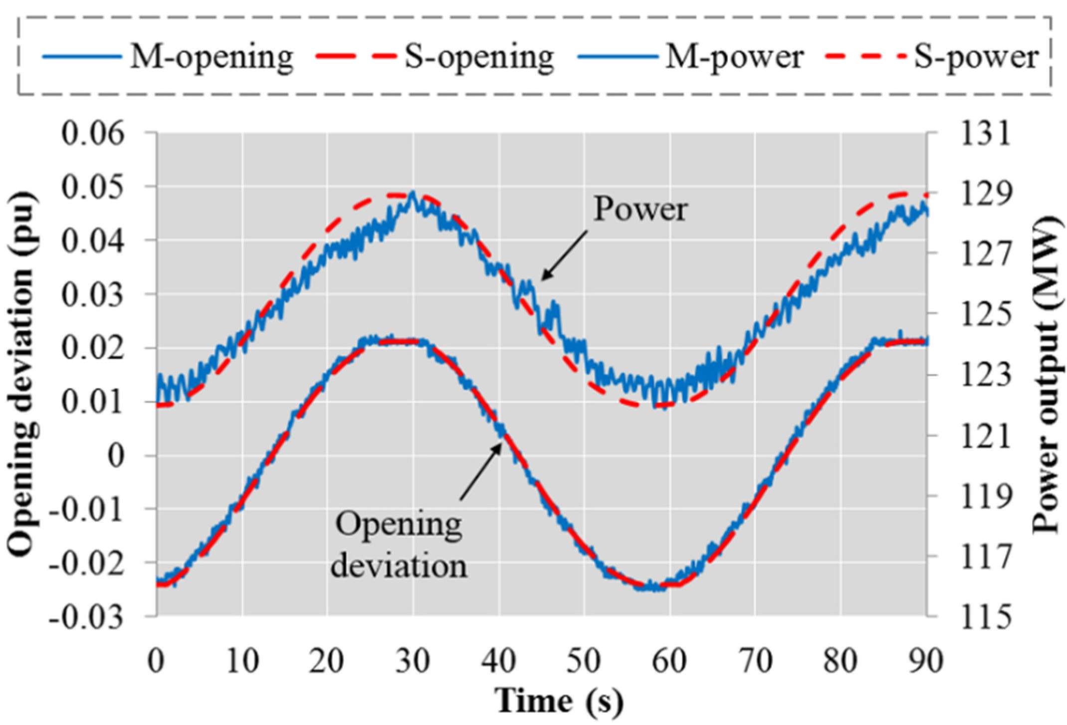
Figure 6. Power output and opening from simulation and measurement under sinusoidal frequency input (Case 1).

Figure 6. Power output and opening from simulation and measurement under sinusoidal frequency input (Case 1).

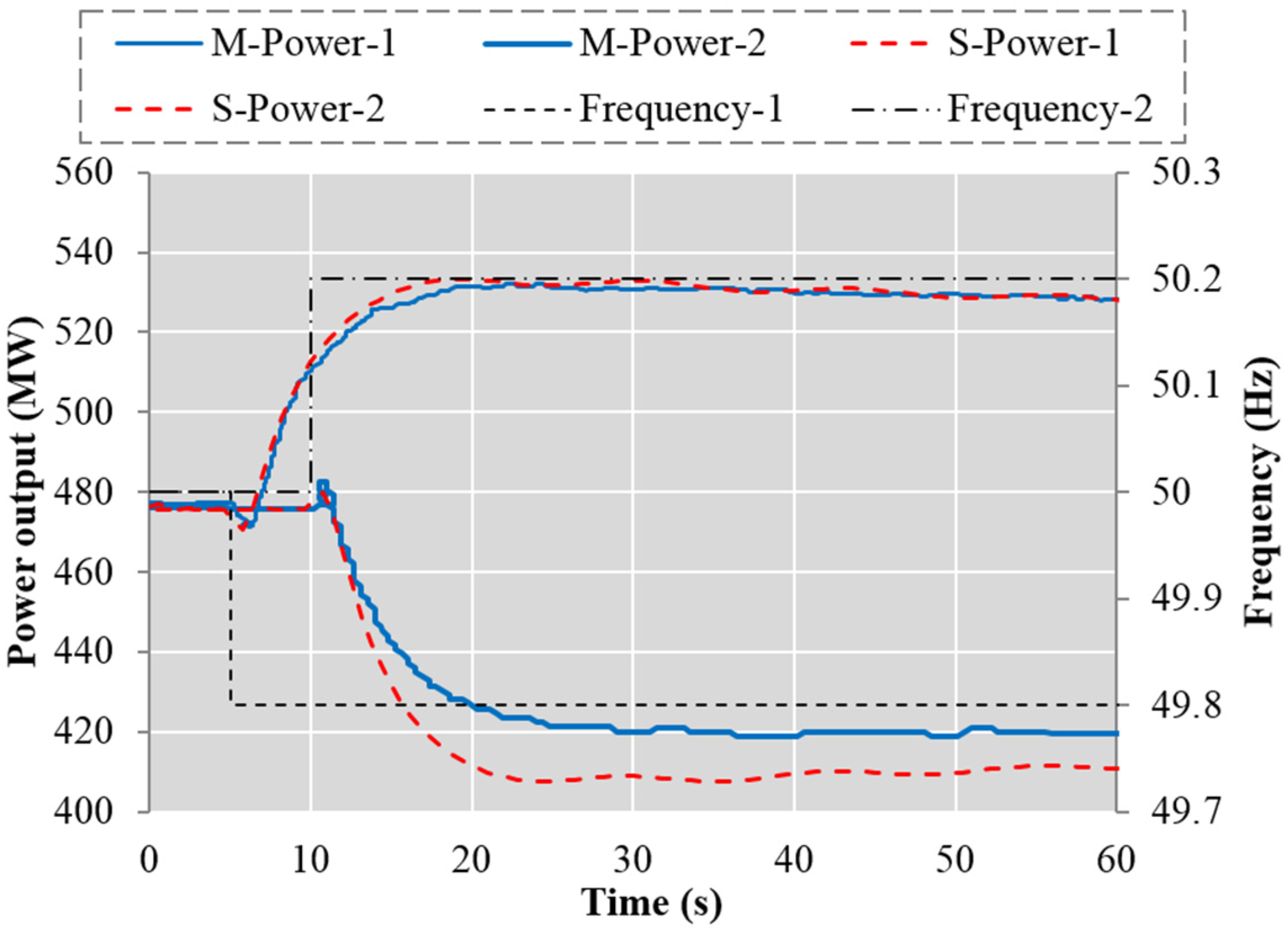
In the figures of this paper, the “M” refers to measurements and the “S” means simulation. Overall, the simulation has a good agreement with measurements. As shown in Figure 6, the effect of backlash is reflected: the opening keeps stable for a short period during the direction change process (e.g., around 28 s). In Figure 7, after the frequency step change, the phenomenon of power reverse regulation caused by water hammer is simulated accurately, as well as the gradual power increase or decrease due to surge (after 20 s in Figure 7). However, the simulation of the power decrease has a lower value than the measurement. This deviation could be ascribed to the characteristic curve, which is normally obtained from the turbine model tests conducted by the manufacturer. To some extent, the on-site measurements inevitably deviate from the simulation which is based on the data from the model tests.

Figure 7. Power from simulation and measurement under step frequency input (Case 2).

Figure 7. Power from simulation and measurement under step frequency input (Case 2).

3.1.2. Isolated Operation

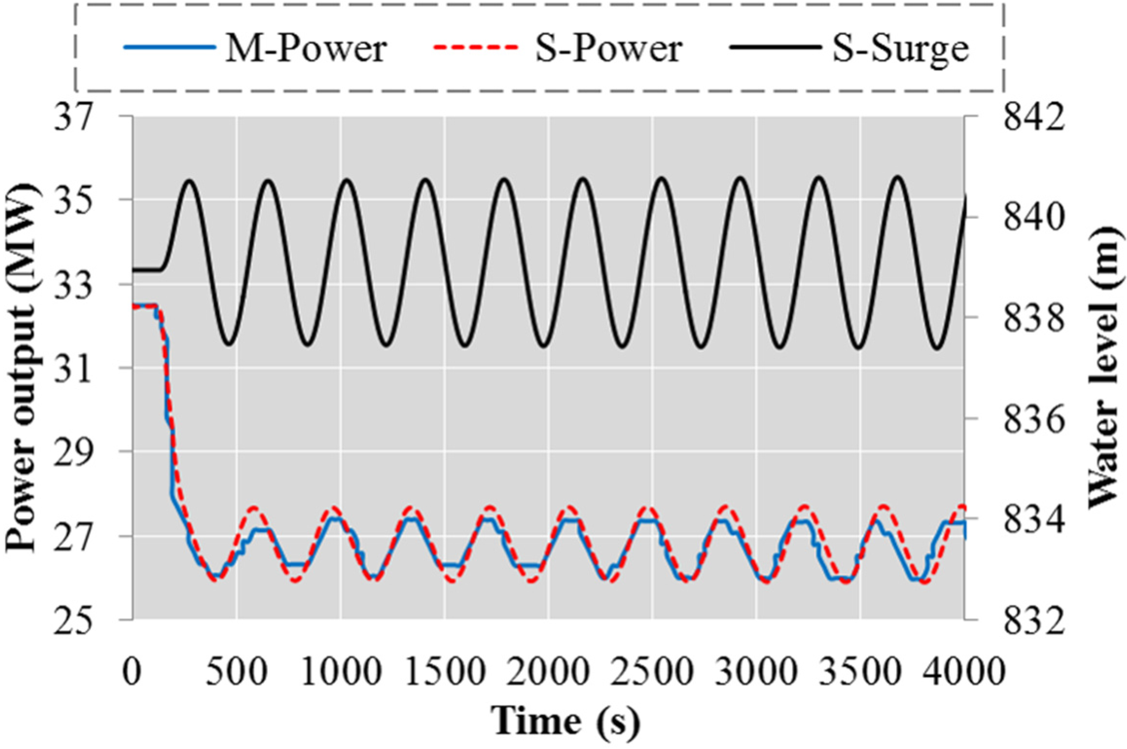
For isolated operation, stability is one of the most crucial aspects. The oscillation after a load step change is examined by simulation and compared with measurements, as shown in Figure 8.

Figure 8. Simulation and measurement of the power oscillation under power control mode (Case 3).

Figure 8. Simulation and measurement of the power oscillation under power control mode (Case 3).

The simulation reflects the real operating condition well: under the power control mode in HPP Case 3, the power oscillates with the surge oscillation under certain governor parameter settings due to a relative small cross section of the surge tank. The simulated period of power oscillations is slightly larger than the measurement value, because of a larger surge period than the actual value. This might be a consequence of small errors in parameters of the waterway system.

3.2. Start-Up and No-Load Operation

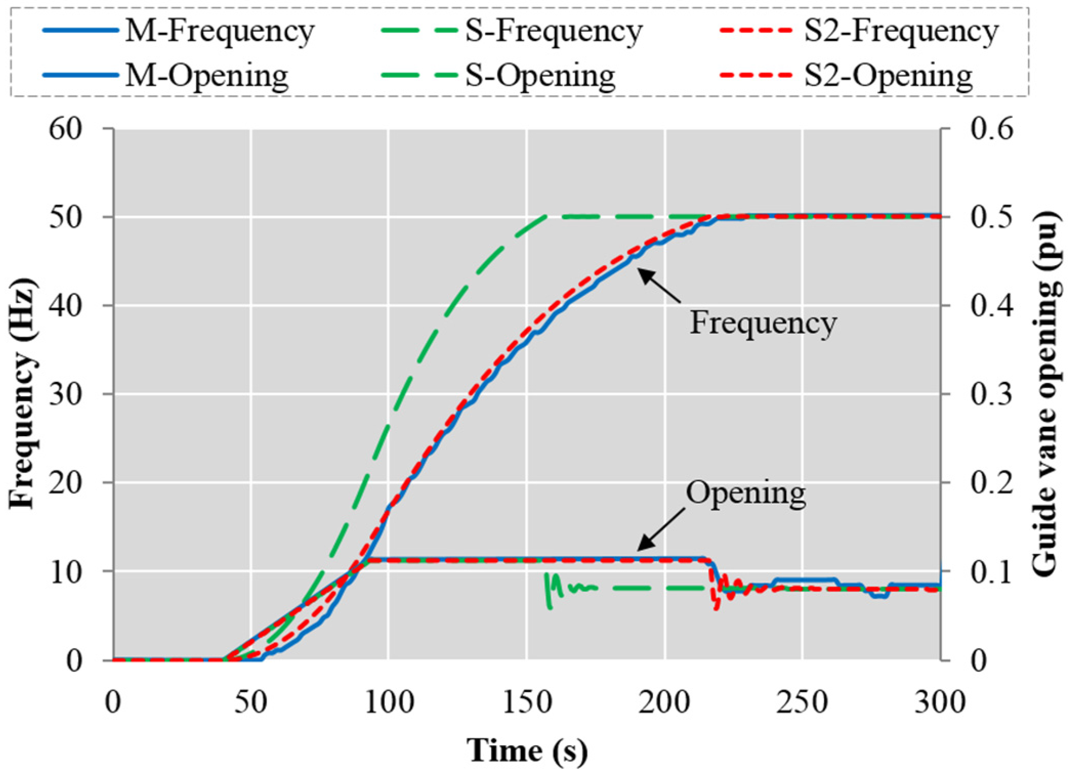
For the start-up process, a rapid and stable increase of the unit speed (generator frequency) is highly important. The start-up process of HPP Case 2 is simulated and compared with measurements, as shown in Figure 9. The switching point from open-loop mode to closed-loop is 100% of the rated speed value. In the simulation with the original characteristic curve of the turbine (S), the simulated frequency increase process is approximately 30% shorter than the measured one, hence the opening from simulation decrease to the no-load opening slightly earlier than the measured opening. Therefore, the curve was modified by decreasing the efficiency. With this revised characteristic curve, the new simulation (S2) fits the measurement well. It demonstrates that the inaccurate simulation mainly hinges on errors in the characteristic curve, which is especially error-prone in the small-opening operation range. Because for the small-opening operation range, the original input data achieved from the characteristic curve is not accurate enough and very sparse, hence it is hard to lead to a good simulation.

Figure 9. Frequency and opening from simulation and measurement during a start-up process (Case 2). The “S” means the simulation with the original characteristic curve of turbine, and the “S2” means the simulation with the modified characteristic curve.

Figure 9. Frequency and opening from simulation and measurement during a start-up process (Case 2). The “S” means the simulation with the original characteristic curve of turbine, and the “S2” means the simulation with the modified characteristic curve.

3.3. Large Disturbance: Load Rejection

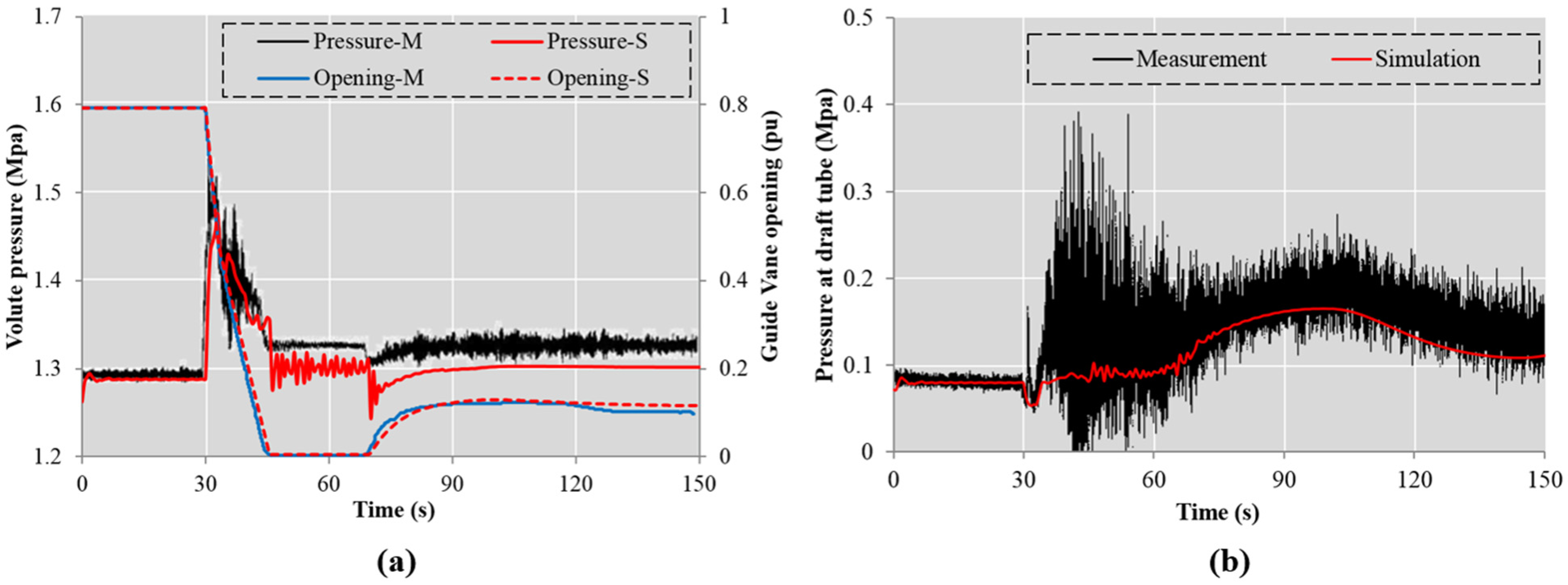
The pressures at the inlet of the volute and in the draft tube are two key indices for the safety of the plant at load rejection. These pressure values are simulated during load rejection, and compared with measurements in HPP Case 4, as demonstrated in Figure 10. The broken-line closure law of the guide vanes is adopted. For the simulated pressure, there is a small static deviation from the measurement after load rejection. It might be due to the water head error caused by the characteristic curve and imprecise parameters of the waterway system.

Figure 10. Simulation and measurement of the (a) guide vane opening and pressure at volute; and (b) pressure at draft tube, during a load rejection process (Case 4).

Figure 10. Simulation and measurement of the (a) guide vane opening and pressure at volute; and (b) pressure at draft tube, during a load rejection process (Case 4).

Moreover, the pulsating pressure at volute and draft tube in the measurement cannot be reproduced by the simulations because of the limitation of the one-dimensional characteristic method. The pressure measurement in the draft tube might also be difficult to compare to modeled values, due the swirl not being modeled in the 1-D modeling approach, making the actual water velocity past the pressure transducer deviate from the mean velocity in an unknown way. Then, as shown in Figure 10a, during the operation period under zero guide vane opening, the simulated pressure oscillates when the measurements show the minimum oscillations. The reason is that during this period, the pressure pulsation is normally large because of the complex unsteady flow; while in the real operation case, the flow rate is larger than the theoretical value, due to the leakage in the turbine actuator. Therefore the measured pressure pulsation becomes smaller than the simulated value.

4. Discussion

The results in Section 3 show that the model can yield trustworthy simulation results for different physical quantities of the unit under various operating conditions. The main error source of the simulation is the characteristic curves of the turbine, from the manufacturer, which directly causes small deviations of power output and affects the rotation speed and pressure values. The reason is that the characteristic curve does not really describe the on-site dynamic process accurately, and the error is especially obvious in the small-opening operation range. Before, start-up simulations were seldom compared with the on-site measurements. The deviation for the start-up process was also found in [5] from the similar results, the difference between the simulated and measured “gate opening” is relatively large. In Section 3.2, a better simulation for start-up process was obtained by changing the overall efficiency of characteristic curve. This simple method is a temporary approach for this stage, it should be replaced by a more advanced and general one to adjust the simulation, as an important future work. What’s more, waterway system parameters might also have errors that impact the simulation.

There are various types of governor systems installed in real HPPs, but most of them are PID (or proportional-integral) controllers and very similar to each other. For example, in some governors, the signal after the droop is only input to the P or PI terms, instead of being input to all of the PID terms. The opening feedback signal before the droop could also be the output after the non-linear mechanical-hydraulic components (saturation, rate limiting and servo). For a concise presentation of the model, only one standard type of PID governor system is described in this paper; while in case studies, the program TOPSYS is flexible and can be modified according to the actual governor conditions.

In general, several function features of the model could be condensed as follows, by comparing with a general MATLAB model, e.g., the hydro turbine model in the Power System Analysis Toolbox (PSAT, an open-source MATLAB toolbox): (1) the model in this paper implements more operation conditions than the PSAT model, which mainly focuses on the small disturbance; (2) as mentioned in Section 1, various hydraulic factors and the characteristic curve are considered in detail, while the PSAT model does not. Therefore, this model could lead to a more sophisticated simulation, especially for the HPP with surge tanks and different units which are sharing the same pipeline; and (3) the TOPSYS is an executable file (.exe) which can operate without installing of MATLAB or other software packages. However, PSAT also has other advantages which are important future works for TOPSYS development, e.g., the comprehensive modelling of power system components and various simulations regarding electrical steady analysis and transient process.

Besides, it is worth mentioning that other advanced versions of TOPSYS were developed or are in development now, to improve the analysis of different components in HPPs and pumped storage plants. These studies focus on following aspects and relates to some important issues in this paper: (1) complete characteristic of pump turbines with space curved surface [18] was researched for a better description of the characteristic curves; (2) 1-D explicit-implicit coupling methods of unsteady flows in pipe networks [22] were studied for a more accurate modeling of complex water way systems; (3) 1-D and 3-D (three-dimensional) coupling approaches for system simulation [23] were developed to overcome limitations of 1-D simulation, enabling the sophisticated modeling of turbines to compute the flow field and pressure in the volute and draft tube.

Furthermore, in terms of hydro power units, this research could also be extended in these points below: (1) a more sophisticated model for electrical components needs to be built to research the interaction between HPPs and power system; (2) modeling and investigation on the dynamic response of HPPs under advanced control methods, instead of typical PID control, are of importance; and (3) other types of turbines, e.g., Kaplan and Pelton, need to be studied.

5. Conclusions

This paper displays a mathematical model of hydro power units, especially a governor system model for different operating conditions, based on the existing basic version of the software TOPSYS, by applying Visual C++. The whole model of the unit consists of ten unknown variables, and ten equations are adopted to describe and analyze the dynamic system. The equation sets for different conditions are presented and discussed in detail. All the essential non-linear factors in the governor system (dead-zone, saturation, rate limiting, and backlash) are also considered.

Based on four engineering cases, the model application is proved reliable for computing different physical quantities of the unit (e.g., guide vane opening, active power, rotation speed, and pressures) by comparing the simulation with on-site measurements of different operating conditions, e.g., start-up, no-load operation, normal operation, and load rejection in different control modes (frequency, opening, and power feedback). Discussion of the error sources is also conducted under each condition.

Finally, the described model is the crucial part of the transient process simulation for the whole power plant. It can be very useful in the design, commissioning, and further study of HPPs, by enabling quick testing to reduce the time for tuning of system parameters and control settings. The model has already been applied effectively in consultant analyses and scientific studies.