Numerical Analysis on the Stability of Hydraulic Fracture Propagation

Abstract

The formation of dense spacing fracture network is crucial to the hydraulic fracturing treatment of unconventional reservoir. However, one difficulty for fracturing treatment is the lack of clear understanding on the nature of fracture complexity created during the treatment. In this paper, fracture propagation is numerically investigated to find the conditions needed for the stable propagation of complex fracture network. Firstly, starting from a parallel fracture system, the stability of fracture propagation is analyzed and a dimensionless number M is obtained. Then, by developing a hydraulic fracturing simulation model based on displacement discontinuity method, the propagation of parallel fractures is simulated and a clear relation between M and the stability of parallel fractures is obtained. Finally, the investigation on parallel fractures is extended to complex fracture networks. The propagation of complex fracture networks is simulated and the results show that the effects of M on complex fracture networks is the same to that of parallel fractures. The clear relation between M and fracture propagation stability is important for the optimization of hydraulic fracturing operation.

1. Introduction

The formation of dense spacing fracture networks is a common occurrence during the hydraulic fracturing treatment of unconventional reservoirs [1,2] and is important to the success of hydraulic fracturing operations. For the design of fracturing operations, one of the difficulties is the lack of clear understanding on the nature of fracture complexity created during fracturing treatment [2]. However, the investigation on the propagation of complex fracture networks is challenging at present. For example, fracture propagation in the field can be observed by methods such as micro seismic mapping and pumping pressure diagnosis, but the details cannot be measured completely by these observation methods. Experiments can be performed in a laboratory [3,4,5], but it is not easy to relate the experiment results to the operation in the field [6]. Comparing with the observation methods and laboratory experiments, numerical modelling is much more flexible. Numerical models can be established according to field conditions and all the details can be exported for analysis. However, the simulation of fracture network propagation is very complex. Proper modelling requires consideration of all the important factors, including natural fractures, rock properties, in-situ stress, fluid properties, injection rate, injection of proppant, etc. Many models in early stages, such as the PK model [7], PKN model [8], KGD mode [9], pseudo-3D models, and planar-3D models [10,11], can only be used in simulating the propagation of fractures with highly idealized geometries. Some traditional methods, such as the finite difference method [12], finite element method [13], extended finite element method [14,15,16], discrete element method [17], have been used in the simulation of fracture network in recent years, but are computationally demanding and are ill-conditioned [17] for the fluid-rock coupling process of hydraulic fracturing. Different from these traditional methods, meshless methods [18,19,20] are free from meshing and with capability to deal with moving boundary conditions. Meshless methods are flexible and accurate in simulating fracture propagation, but have not been in used in simulating the complex fracture network propagation in hydraulic fracturing. Displacement Discontinuity Method (DDM) [21,22,23,24], which is a kind of boundary element method, is more appropriate for the simulation of complex fracture networks and has been used by more and more researchers [2,25,26,27,28,29]. The propagation of complex fracture networks can be simulated within shorter CPU time because the rock matrix is not discretized. Moreover, the fracture aperture can be calculated with higher precision because a volume integral is not needed.

However, even with numerical modelling, the investigation of complex fracture networks is still in its infancy due to the complexity of the propagation process. The propagation of complex fracture networks depends on many factors. Much attention from the hydraulic fracture modeling community has focused on the effects of these influence factors on the propagation process. For example, Nagel, et al. [30] simulated the propagation of a large number of fractures with 3DEC to investigate the effects of injection rate and viscosity on tensile and shear failure. The results show that higher injection rates favor tensile failure while the lower injection rates and lower viscosity favors the creation of shear fracture. Riahi and Damjanac [31] performed a series of comparative studies with UDEC to establish the effects of injection rates, the connectivity and size distribution of natural fractures on a stimulated area. It was found that higher injection rates resulted in smaller stimulated shear area. Fu, Johnson, and Carrigan [17] simulated the fracturing process with dozens of natural fractures to investigate the effects of principal stress orientation and stress anisotropy. It was found that fracture networks propagate along the maximum principle stress direction and the fracture network is more complex when the stress is isotropous. McClure and Horne [32] investigated the conditions required for shear stimulation and showed that stimulations may occur through a mixture of the opening and sliding of preexisting fractures and the propagation of new fractures. Zhang and Jeffrey [26] simulated the fracturing process under two injection types and it was found that equal rate injection is better than equal pressure injection in creating complex fracture network. Zhuang, et al. [33] investigated the feasibility of utilizing hard rock for compressed air energy storage. For rock cavern with fracture, higher fluctuation of pressure and temperatures are found, which is unfavorable for system stability. Rabczuk, et al. [34,35,36,37] proposed a meshless method that is able to treat the nucleation of fractures and complex patterns involving fracture branching and crossing in a simple and effective way. Aside from the works above, the propagation of complex fracture networks has also been investigated by many other researchers [2,25,27,28,33]. To sum up, the effects of many factors on the propagation of complex fracture networks have been investigated. However, most of the results on complex fracture network are descriptive. The descriptive results are helpful in telling us how to achieve complex fracture networks, but is not easy to be used in determining the optimal fracturing parameter.

One of the difficulties for the investigation on the propagation of complex fracture networks is the large number of influence factors. The propagation of complex fracture network depends on so many factors that it is very difficult to quantify the effects of all these factors just by numerical modelling. Fortunately, the effects of these factors are not independent. For example, Guo, et al. [38] investigated the effects of flow rate and fluid viscosity on fracturing process and suggested that the influence of flow rate and viscosity can be expressed as their product and thus there is no need to investigate the effects of viscous coefficient and injection rate individually. That is, the appropriate theoretical analysis is helpful in finding the key factors and in reducing the number of influence factors. Therefore, to get clear relations between the influence factors and the propagation of complex fracture networks, hydraulic fracturing process is theoretically analyzed before numerical modelling in this paper. First, by analyzing the propagation of parallel fracture systems, a dimensionless number that account for the stability of the propagation is obtained. Both fluid properties and rock properties are in consideration during the derivation of the dimensionless number. And then, by simulating the propagation of parallel fractures and complex fracture networks, the effects of the dimensionless number is quantified.

2. The Propagation of Parallel Fracture

2.1. The Propagation Stability

Consider a possible idealized picture of fracture system development in unconventional reservoir [39]. The first set of fractures, roughly orthogonal to the borehole, are formed at the locations of casing perforations. Then, secondary fractures of denser spacing, roughly orthogonal to the primary fractures, are formed. For theoretical purposes, the propagation of complex fracture networks can be idealized to multiple stages of parallel fracture propagation. The formation of dense spacing fracture networks requires the stable propagation of these parallel fractures without localization, i.e., the lengths of each fracture keep equal during propagation [39]. The fracture lengths could keep equal only when the propagation speed of the shorter fractures is no slower than that of the longer fractures, which requires the energy consumption for fracture propagation is less for the shorter fractures. For the two sets of fractures as shown in Figure 1, a₁ and a₂ are the lengths of the two sets of fractures respectively and a₁ < a₂, the length difference $\delta a=\left|a_2-a_1\right|$ will not increase when

$$\frac{\partial F}{\partial a_1}<\frac{\partial F}{\partial a_2}$$

(1)

where F is the energy consumption, i.e., the energy consumption for the propagation of the shorter fractures is less than that of the longer fractures. The analytical expression of F is difficult to be given because it depends on many factors, for example, the fracture length, fracture aperture, viscosity of fluid, and most importantly, interactions between fractures. Therefore, the energy consumption will be analyzed under very ideal conditions in this part. The aim of the analysis is to find how these factors affect the stability of fracture propagation and which is the key factor.

The first kind of energy consumption is the fracture surface energy, which satisfies

$$\frac{\partial F}{\partial a_1}=\frac{\partial F}{\partial a_2}=\mathrm{\Gamma }$$

(2)

where $\mathrm{\Gamma }$ is the fracture energy. Therefore, the fracture surface energy does not contribute to the stability of fracture propagation, which is the same as that of cooling fractures [39].

The second kind of energy consumption is the viscous dissipation of fluid. Assuming the pressure gradient caused by fluid viscosity equals ∂p/∂y, then the pressure drop along the fracture equals a∂p/∂y. Therefore, when a fracture extends a small length δa, the energy input needed is proportional to aδa ∂p/∂y, then

$$\frac{\partial Q}{\partial a_1}\propto a_1\frac{\partial p}{\partial y},\frac{\partial Q}{\partial a_2}\propto a_2\frac{\partial p}{\partial y}$$

(3)

where Q is the viscous dissipation of fluid. It is clear that

$$\frac{\partial Q}{\partial a_1}<\frac{\partial Q}{\partial a_2}$$

(4)

i.e., the viscous dissipation is stronger for the longer fractures and the Equation (1) is satisfied by U. Therefore, fluid viscosity helps to keep the stability.

The third kind of energy is the strain energy of the elastic solid. Different from fracture energy and viscous dissipation, the strain energy is conservative. However, the strain energy could be treated as energy consumption when neglecting the shrink of fracture, which is a reasonable assumption as fluid pressure increases with fluid injection. Moreover, the shrinking of a fracture can be partly suppressed by the pumping of proppant. The analytic expression of the strain energy can be given in the special circumstance when a << s, where a is the fracture length and s is the fracture spacing. The stress interaction between fractures is ignorable when a << s, then fracture aperture w satisfies [40]

$$w\left(r\right)=\frac{4\left(1-{\nu }^2\right)}{E}pa\sqrt{1-\frac{{\left(a-r\right)}^2}{a^2}}$$

(5)

where E is Young’s modulus, ν is Poisson’s ratio, p is the fluid net pressure, r is the distance to the fracture tip. Considering the stress intensity factor, K_I can be calculated by the fracture aperture near fracture tip [41]

$$K_I\approx \frac{E}{4\left(1-{\nu }^2\right)}w\left(r\right)\sqrt{\frac{2\text{π}}{r}}$$

(6)

The fluid pressure can be estimated by Equations (5) and (6),

$$p\approx \frac{K_{IC}}{\sqrt{2\text{π}a}}$$

(7)

i.e., fluid pressure decreases with the propagation of fracture at initial stage, where K_IC is the tensile mode fracture toughness. As the strain energy U is equal to the energy inputted E_input by injecting fluid quasi-statically and ∂E_input/∂V = p, so we have

$$\frac{\partial U}{\partial V}=p$$

(8)

where U is the strain energy, V is fracture volume, which is proportional to a² at initial stage. Considering a₁ < a₂, we have

$$\frac{\partial U}{\partial a_1}>\frac{\partial U}{\partial a_2}$$

(9)

that is, the Criterion (1) is not satisfied by U when a<<s. The analytic expression of U cannot be given when the fractures are much longer. However, due to the opening of the longer fracture, the in situ stress at the tip of the shorter fracture is bigger than the longer one, i.e., higher fluid pressure is needed for the growth of the shorter fracture. Therefore, the energy consumption for the propagation of the shorter fracture is bigger than the longer one. That is, the Equation (9) still exists when the fractures are longer. In conclusion, the propagation is not stable when considering the strain energy.

Figure 1. Two sets of hydraulic fractures starting from the same wellbore.

Figure 1. Two sets of hydraulic fractures starting from the same wellbore.

From the analysis above, it is clear that the propagation stability of parallel fractures depends on two mechanisms, i.e., the viscosity of fluid and the elasticity of rock. Moreover, the effects of the two mechanisms are opposite. The viscosity of fluid helps to keep the stability while the elasticity of solid leads to the instability. Therefore, the propagation stability of hydraulic fractures depends on the competition between these two mechanisms.

2.2. The Dimensionless Number

The competition between the viscosity of fluid and the elasticity of rock can be quantified by defining a dimensionless number Μ, which is the ratio between the fluid pressure caused by viscosity and the initiation pressure of rock. For a system of parallel fractures with fracture spacing equal to s, the fluid pressure caused by viscosity can be quantified by the pressure drop within characteristic length s. As the volumetric flux q of fluid in fracture is given by [26]

$$q=-\frac{w^3}{12\text{μ}}\nabla p$$

(10)

then the drop of fluid pressure $\mathrm{\Delta }p$ equals

$$\mathrm{\Delta }p=\frac{12q\text{μ}s}{w^3}$$

(11)

where μ is fluid dynamic viscosity, $\nabla p$ is the gradient of fluid pressure, w is fracture aperture. For the parallel fracture system, the fracture aperture satisfies

$$w\propto \frac{ps}{E}$$

(12)

where p is the net pressure of fluid, E is the Young’s modulus of rock. As there is only type I failure in the parallel fracture system, a fracture extends when

$$K_I\ge K_{IC}$$

(13)

where K_I is the tensile mode stress intensity factor, K_IC is the fracture toughness. K_I can be calculated by Equation (6), then we have

$$K_I\propto \frac{Ew}{\sqrt{s}}$$

(14)

Considering Equation (13), then

$$w\propto \frac{K_{IC}\sqrt{s}}{E}$$

(15)

Considering Equation (11), then

$$\mathrm{\Delta }p\propto \frac{q\text{μ}{E}^3}{\sqrt{s}{K_{IC}}^3}$$

(16)

Considering Equations (12) and (15), we have

$$p_C\propto \frac{K_{IC}}{\sqrt{s}}$$

(17)

where p_C is the initiation pressure, which is the net fluid pressure needed for fracturing the rock. Then we have

$$\frac{\mathrm{\Delta }p}{p_C}\propto \frac{q\text{μ}{E}^3}{{K_{IC}}^4}$$

(18)

As the net pressure of fluid is proportional to the elastic energy of rock and $\mathrm{\Delta }p$ is caused by the viscosity of fluid, the dimensionless number Μ can be defined as

$${\rm M}\equiv \frac{q\text{μ}{E}^3}{{K_{IC}}^4}$$

(19)

It is clear that M represents the competition between the viscous dissipation of fluid and the strength of rock deformation.

The dimensionless number M is closely related to the stability of the fracture propagation. However, it is difficult to know how the stability varies with M. Moreover, the theoretical analysis above is implemented based on very ideal circumstances. To investigate the propagation stability of fracture under more general circumstances and to get the clear relation between M and the stability, numerical modelling will be implemented in the following sections.

3. Numerical Model

A DDM based model is developed in this paper. As a kind of boundary element method, DDM solves fracture aperture with very high precision because the theoretical solution of elastic mechanics is directly used [40]. Therefore, the competition between fluid viscosity and solid elasticity can be accurately evaluated.

The following assumptions are used in the model:

(1)

The domain of rock matrix is infinite and the rock matrix is homogeneous, isotropous, linear elastic [40].

(2)

The rock matrix is impermeable [6,26,42].

(3)

The fluid is Newtonian [6,26,42].

(4)

The flow in fracture system is single phase and laminar [6,26,42].

The elastic equilibrium equations for a system of N fracture elements are [26]:

$$\begin{array}{l}{\text{σ}}_n\left(x\right)-{\text{σ}}_1\left(x\right)={\displaystyle \sum _{r=1}^N{\displaystyle {\int }_0^{l_r}\left[G_{11}\left(x,s\right)w\left(s\right)+G_{12}\left(x,s\right)\nu \left(s\right)\right]K\left(x,s\right)ds}}\\ {\tau }_s\left(x\right)-{\text{τ}}_1\left(x\right)={\displaystyle \sum _{r=1}^N{\displaystyle {\int }_0^{l_r}\left[G_{21}\left(x,s\right)w\left(s\right)+G_{22}\left(x,s\right)\nu \left(s\right)\right]K\left(x,s\right)ds}}\end{array}$$

(20)

where x = (x, y) is the coordinate, w is the normal displacement discontinuity, v is the shear displacement discontinuity, l_r is the length of fracture r, σ_n is the normal stress and τ_s is the shear stress, obeying Coulomb’s frictional law characterized by the coefficient of friction λ

$$\left|{\text{τ}}_s\right|\le {\text{λσ}}_n$$

(21)

that can act in parts of fractures that are in contact, and vanishes along the separated parts. Along the opened fracture portions, we have σ_n = p_f. In addition, σ₁ and τ₁ are the normal and shear stresses along the fracture direction respectively caused by far-field stress. G_ij are the hyper singular Green’s functions, which are proportional to the plane strain Young’s modulus [26]. K is the three dimensional correction coefficient proposed by Olson [43]. Using the parameters given by Wu and Olson [44], K can be written as

$$K\left(x_1,x_2\right)=1-\frac{d^3}{{\left[d^2-{\left(h/2\right)}^2\right]}^{3/2}}$$

(22)

where h is layer thickness perpendicular to the simulation plain, d is the distance between points x₁ and x₂.

The fluid flow in fracture system follows the Equation (10) and the global mass balance requires

$$\frac{\partial }{\partial t}\left(\frac{\text{δ}{v}_f}{\text{δ}L}\right)+\nabla q=0$$

(23)

where v_f is fluid volume, which is no bigger than fracture volume. L is fracture segment length, $\nabla q$ is the gradient of flow rate along fracture.

The fracture growth is based on the maximum hoop stress criterion, with the maximum mixed-mode intensity factor reaching a critical value [26,45]

$$\frac{1}{2}\cos \frac{{\text{θ}}_{\text{0}}}{\text{2}}\left[K_I\left(1+\cos {\text{θ}}_0\right)-3K_{II}\sin {\text{θ}}_0\right]=K_{IC}$$

(24)

where K_I and K_II are stress intensity factors, K_IC is tensile mode fracture toughness, θ is the fracture propagation direction relative to the current fracture orientation and satisfies [26,45]

$$K_I\sin \text{θ}+K_{II}\left(3\cos \text{θ}-1\right)=0$$

(25)

The interaction between hydraulic and natural fractures is also simulated based on the above criterion. When a hydraulic fracture encounters a natural fracture, it will across the natural fracture when the tensile stress is strong enough. Therefore, a virtual fracture element is added at another side of the natural fracture to check the stress condition. The stress intensity factor of the virtual fracture is calculated with the in situ stress at the tip of the virtual fracture and the fluid pressure at the crossing point. The hydraulic fracture will across the natural fracture when the Equations (24) and (25) are satisfied. This method for dealing with fracture interaction has clear physical background and is easily implemented under the framework of DDM.

For validation, we refer for comparison to the model of Wu and Olson [28] for the fracture configurations of a single horizontal wellbore with two initial fractures (Figure 2a) and two horizontal wellbores with one fractures each (Figure 2b). These are the most classic configurations and have been simulated in many works [2,27,28,30,44,46]. The correct simulation of these configurations requires the precisely solving of the stress field and fluid pressure, and the correct calculating of the stress intensity factor. These two configurations are simulated with the parameters listed in Table 1, which is the same to that of Wu and Olson [28]. The results are shown in Figure 3. For the initial configuration as shown in Figure 2a, the two fractures propagate away from each other. For the initial configuration as shown in Figure 2b, the two fractures grow toward each other. In summary, our model compares favorably with previous models.

Figure 2. Two initiation fractures in (a) a horizontal wellbore and (b) two horizontal wellbores. Blue lines represent horizontal wellbores, and red lines represent initial fractures.

Figure 2. Two initiation fractures in (a) a horizontal wellbore and (b) two horizontal wellbores. Blue lines represent horizontal wellbores, and red lines represent initial fractures.

Table 1. Input parameters (After Wu and Olson [28]).

Parameter	Value
q	8.8 × 10−4 m3/s/m
μ	1.0 cP
E	3.0 × 1010 Pa
Poisson’s Ratio	0.35
h	120 m
KIC	1.0 × 106 Pa.m0.5
Far-field stress	σx = σy = 47 MPa

Table 1. Input parameters (After Wu and Olson [28]).

Parameter	Value
q	8.8 × 10−4 m3/s/m
μ	1.0 cP
E	3.0 × 1010 Pa
Poisson’s Ratio	0.35
h	120 m
KIC	1.0 × 106 Pa.m0.5
Far-field stress	σx = σy = 47 MPa

Figure 3. Comparison of propagation paths for initiation fractures in (a) a horizontal wellbore and (b) two horizontal wellbores. The line width represents the fracture aperture.

Figure 3. Comparison of propagation paths for initiation fractures in (a) a horizontal wellbore and (b) two horizontal wellbores. The line width represents the fracture aperture.

4. Numerical Analysis

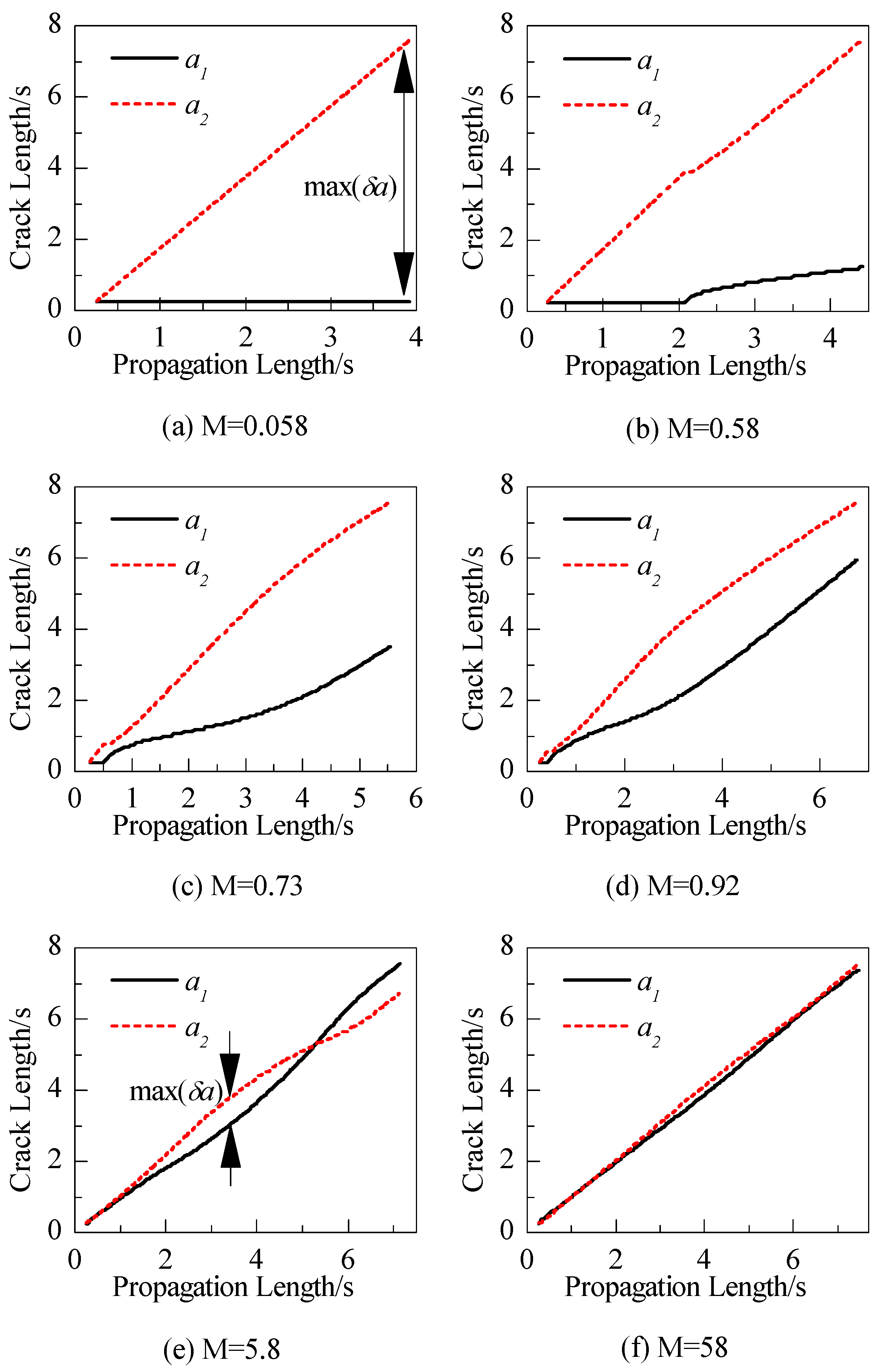
4.1. Parallel Fracture

The propagation of the parallel fracture system as shown in Figure 1 is first simulated. The aim of the simulation is to investigate the conditions needed for the controlling of length difference during the propagation. There are infinite number of fractures in Figure 1. However, the infinite number of fractures can be divided into two periodically appeared sets. Therefore, with periodical boundary condition at the left and right side, the infinite number of fractures in Figure 1 can be simulated by only two fractures as shown in Figure 4. The periodical boundary condition is implemented by calculating the induced stress of a fracture as the fracture appears periodically at the left and right sides.

Figure 4. The simulation setting.

Figure 4. The simulation setting.

Fluid is injected into the wellbore with the constant rate q, which is also the sum of the injection rate into the two fractures. The allocation of flow rate depends on the pressure profile along the wellbore. Therefore, the injection rates for the two fracture may be different and may vary during the simulation. However, as the conductance of the wellbore is much bigger than the fractures, the pressure along the wellbore is approximately uniform and the inlet pressures of the two fractures are approximately equal.

The in situ stress is set to be isotropic. The layer thickness h in Equation (22) is set to be infinite and three dimensional effect is ignorable. A small initial length difference is assigned to the system because small disturbance always exists in actual case. The initial lengths of the fractures are a_1,0 = 0.25 s, a_2,0 = 0.275 s, where s is the fracture spacing. The propagation is simulated under the parameters listed in Table 2. The variations of the lengths of the two fracture sets, a₁ and a₂, are outputted for analysis. The simulation is ended when a₁ > 7.3 s or a₂ > 7.3 s.

The propagations of the parallel fractures under different values of M are shown in Figure 5. The propagation length is defined as the average length of the two fractures. When Μ = 0.058, one fracture propagates while the propagation of another fracture is totally suppressed. When Μ = 0.58, the shorter fracture begins to propagate when the length of another equals to 4s approximately. When Μ = 0.73 and Μ = 0.92, the initially shorter fracture begins to propagate almost at the same time with the longer fracture and the length difference increases with propagation length. When Μ = 5.8 and Μ = 58, the two fractures propagate simultaneously, and the length difference is smaller than the results when M is smaller. The propagation is leaded by the two fractures alternately as the shorter fracture could always catch up the longer one. Therefore, the lengths of the two fractures will keep equal approximately during the propagation process. In conclusion, the stability of fracture propagation increases with M.

Table 2. Input parameters.

Parameter	Value
q	In range [1.0 × 10−4, 1.0 × 10−1] m3/s/m
μ	0.1 cP
M	In range [0.058, 58]
E	1.8 × 1010 Pa
Poisson’s Ratio	0.2
h	Infinite
KIC	1.0 × 106 Pa.m0.5
Far-field stress	σx = σy = 5.0 × 107 Pa

Table 2. Input parameters.

Parameter	Value
q	In range [1.0 × 10−4, 1.0 × 10−1] m3/s/m
μ	0.1 cP
M	In range [0.058, 58]
E	1.8 × 1010 Pa
Poisson’s Ratio	0.2
h	Infinite
KIC	1.0 × 106 Pa.m0.5
Far-field stress	σx = σy = 5.0 × 107 Pa

Figure 5. The paths of fracture length under different values of M. (a) M = 0.058, (b) M = 0.58, (c) M = 0.73, (d) M = 0.92, (e) M = 5.8, (f) M = 58.

Figure 5. The paths of fracture length under different values of M. (a) M = 0.058, (b) M = 0.58, (c) M = 0.73, (d) M = 0.92, (e) M = 5.8, (f) M = 58.

Figure 6 shows the variation of max(δa) with M, where max(δa) is the maximum fracture length difference during the simulation, as illustrated in Figure 5a,e. When M < 0.2, max(δa) = 7.3 s, i.e., there is no propagation for the initially shorter fracture. It is clear that max(δa) decreases with Μ when M > 0.2. Moreover, the decrease is not uniform. When M∈[0.2,1.0], the decrease of max(δa) is very steep. By contrast, when M > 1, the decrease of max(δa) is slow. That is, the stability of the propagation increases rapidly with M when M∈[0.2,1.0] while the increase of the stability is very limited when M > 1.0. Therefore, we should try our best to increase the value of M to improve the propagation stability when M < 1.0 during the hydraulic fracturing operation.

Figure 6. The variation of length difference with M.

Figure 6. The variation of length difference with M.

4.2. Complex Fracture Network

The investigation on parallel fractures is extended to complex fracture network in this part. The propagation processes of complex fracture network under the same value of M as the points (a)–(d) shown in Figure 6 are simulated.

The natural fracture network is created by a discrete fracture network model [31] with the parameters listed in Table 3. The fracture length follows a power law distribution [31], i.e., n(l)$\propto$l^−α, where n is the occurrence of a fracture with length l, α is a site specific value [31]. Two sets of fractures are in consideration. The angles between the fractures and the positive direction of x axis equal to π/3 and 2π/3 respectively. P21 is used to measure the fracture density [31] and P21 = 6.0 m⁻¹ in Figure 7. The poorly connected natural fracture network is used so that the fracturing process is dominated by the propagation of hydraulic fracture, which is similar to the parallel fracture system. However, because fracture energy has no effect on the propagation stability, the results are similar to that of a well-connected natural fracture network [39].

Fluid is injected with constant rate from the center of the simulation region. The value of M cannot be calculated directly by Equation (19) because q in Equation (19) refers to the flow rate in single fracture. Given the injection rate q_inj, q is calculated by q = q_injs/L, where s is the average spacing between natural fractures and L is the width of the simulation region. The rock and fluid properties are equal to the simulation of parallel fractures in Section 4.1. The in situ stress anisotropy equals to 0.5 MPa with the direction of maximum principle stress shown in Figure 7. The three dimensional effect is considered and the layer thickness h in Equation (22) is set to be 0.5 m. The simulation is finished when any hydraulic fracture reaches the boundary of the simulation region.

Figure 7. The final fracture configurations under different values of M. Fracture width is represented by curve width and fluid net pressure is represented by color. (a) M = 0.18, (b) M = 0.58, (c) M = 1.8, (d) M = 5.8.

Figure 7. The final fracture configurations under different values of M. Fracture width is represented by curve width and fluid net pressure is represented by color. (a) M = 0.18, (b) M = 0.58, (c) M = 1.8, (d) M = 5.8.

Figure 7 shows the final configurations of the complex fracture network under different values of M. When M = 0.18, as in Figure 7a, a dominated fracture grows from center along the maximum principle stress direction. Meanwhile, the growths of all other fractures are suppressed. The fluid pressure is nearly uniform at most parts of the hydraulic fractures. This implies the fluid viscosity is very weak during the fracturing treatment. Only one fracture propagates with fluid injection, which is similar to that of the parallel fracture system when M is very small. When M = 0.58, as in Figure 7b, more fractures propagate with fluid injection because fluid viscosity is stronger. When M = 1.0 and M = 5.8, as shown in Figure 7c,d, a large number of fractures grow from the injection point simultaneously along different directions and an elliptic shaped fracturing zone is formed. The stimulated area is bigger than that of M = 0.18. The fluid pressure decreases from the injection point to the boundary of the simulation region, which implies the fluid viscosity is much stronger than that of M = 0.18.

The behavior of complex fracture networks shows a remarkable similarity with that of parallel fracture system:

(1)

The complexity of fracture network increases with M while max(δa) decreases with M.

(2)

The increment of the fracture network complexity is very significant when M increases from 0.58 to 1.8. Be similarly, the decrease of max(δa) is very significant when M increases from 0.58 to 1.8.

(3)

The variations of both max(δa) and fracture network complexity are not significant when M increases from 1.8 to 5.8.

These results indicate that the stability of parallel fracture system is equivalent to that of complex fracture network. Therefore, the quantitative results obtained from a parallel fracture system are applicable to complex fracture network.

Table 3. Input parameters.

Parameter	Value
Model Width and Height	4.0 m
P21	6.0 m−1
α	3
Fracture Angle	π/3 and 2π/3
Maximum Fracture Length	0.3 m
Minimum Fracture Length	0.1 m
Layer thickness h	0.5 m
Far-field stress	σmax = 5.0 × 107 Pa
Far-field Stress Anisotropy	0.5 MPa
Maximum Principle Stress Angle	5π/6

Table 3. Input parameters.

Parameter	Value
Model Width and Height	4.0 m
P21	6.0 m−1
α	3
Fracture Angle	π/3 and 2π/3
Maximum Fracture Length	0.3 m
Minimum Fracture Length	0.1 m
Layer thickness h	0.5 m
Far-field stress	σmax = 5.0 × 107 Pa
Far-field Stress Anisotropy	0.5 MPa
Maximum Principle Stress Angle	5π/6

5. Discussion and Conclusions

In this work, the stability of hydraulic fracture propagation in unconventional reservoir is analyzed. A dimensionless number M is deduced to account for the stability. It must be noted that the analysis is based on very ideal assumptions, for example, the parallel fracture system, the constant pressure gradient caused by viscosity. The real fracturing process is too complex to be investigated just by theoretical analysis. Therefore, numerical simulation is implemented to find the clear relation between M and the propagation stability.

The dimensionless number M is one of the most important factors that influence the propagation of the fracture network, but not the only one. There are many other factors which have great effects on hydraulic fracturing. For example, as discussed by Bazant, et al. [39], the pumping of proppant helps to prevent the instability by preventing the close of fractures. The in situ stress is also important, the fractures tends to propagate along the maximum principle stress direction. Therefore, the length difference of fractures will be bigger and thus the propagation tend to be instable when the anisotropy of in situ stress is stronger. The brittleness of the rock is important, but the effects of brittleness have been considerate in the definition of M. Considering the Equation (19), the brittleness index B related to hydraulic fracturing could be defined as

$$B=\frac{E^3}{K_{IC}^4}$$

(26)

then the dimensionless number M can be expressed as M = qμB. From the definition of B above, it is clear that the brittleness index B is not just the simple ratio of rock elastic and rock strength. By contrast, the effects of rock brittleness on the fluid-rock coupling process of hydraulic fracturing are closely related to the brittleness index defined as Equation (26). Therefore, we suggest the Equation (26) can be used in quantifying the brittleness of rock on fracturing process other than the existed brittleness indexes, such as the brittleness indexes related to the rock strength, stress-strain curve, loading and unloading test, hardness and mineralogical composition, etc., which were not proposed for the hydraulic fracturing process.

The investigation on the stability of hydraulic fractures shows that:

(1)

The competition between fluid viscosity and solid elasticity, which can be quantified by the dimensionless number M, is one of the controlling factors of the stability of hydraulic fracture propagation.

(2)

The stability of the parallel fracture propagation increases rapidly with M when M∈[0.2,1.0] and increases slowly with M when M > 1.0.

(3)

The propagation of the parallel hydraulic fracture is stable and the two sets of fractures extend alternately when M > 1.0.

(4)

The behavior of complex fracture networks is the same to that of parallel fractures under the same value of M.

(5)

For formations with poorly connected natural fracture network, a complex fracture network can be formed when M > 1.0 while only a single dominated fracture propagates when M < 0.2.

References

1. Maxwell, S.; Urbancic, T.; Steinsberger, N.; Zinno, R. Microseismic Imaging of Hydraulic Fracture Complexity in the Barnett Shale. In Proceedings of the SPE Annual Technical Conference and Exhibition, San Antonio, TX, USA, 9 September–2 October 2002.
2. Weng, X. Modeling of complex hydraulic fractures in naturally fractured formation. J. Unconv. Oil Gas Resour. 2015, 9, 114–135. [Google Scholar] [CrossRef]
3. Meng, Q.; Zhang, S.; Guo, X.; Chen, X.; Zhang, Y. A primary investigation on propagation mechanism for hydraulic fracture in glutenite formation. J. Oil Gas Technol. 2010, 32, 119–123. [Google Scholar]
4. Bunger, A.P.; Gordeliy, E.; Detournay, E. Comparison between laboratory experiments and coupled simulations of saucer-shaped hydraulic fractures in homogeneous brittle-elastic solids. J. Mech. Phys. Solids 2013, 61, 1636–1654. [Google Scholar] [CrossRef]
5. Huang, H.; Zhang, F.; Callahan, P.; Ayoub, J.A. Fluid injection experiments in 2d porous media. SPE J. 2012, 17, 903–911. [Google Scholar] [CrossRef]
6. McClure, M.; Horne, R. Characterizing Hydraulic Fracturing with a Tendency-for-Shear-Stimulation Test. SPE Reserv. Eval. Eng. 2014, 17, 233–243. [Google Scholar] [CrossRef]
7. Perkins, T.; Kern, L. Widths of hydraulic fractures. J. Petrol. Technol. 1961, 13, 937–949. [Google Scholar] [CrossRef]
8. Nordgren, R. Propagation of a vertical hydraulic fracture. Soc. Pet. Eng. J. 1972, 12, 306–314. [Google Scholar] [CrossRef]
9. Geertsma, J.; de Klerk, F. Rapid method of predicting width and extent of hydraulically induced fractures. J. Pet. Technol. (United States) 1969, 2, 1571–1581. [Google Scholar] [CrossRef]
10. Lee, J. Three-dimensional modeling of hydraulic fractures in layered media: Part I—Finite element formulations. J. Energy Resour. Technol. 1990, 112. [Google Scholar] [CrossRef]
11. Siebrits, E.; Peirce, A.P. An efficient multilayer planar 3d fracture growth algorithm using a fixed mesh approach. Int. J. Numer. Methods Eng. 2002, 53, 691–717. [Google Scholar] [CrossRef]
12. Nagel, N.B.; Sanchez-Nagel, M. Stress Shadowing and Microseismic Events: A Numerical Evaluation. In Proceedings of the SPE Annual Technical Conference and Exhibition, Denver, CO, USA, 30 October–2 November 2011.
13. Rahman, M.M.; Rahman, S.S. Studies of hydraulic fracture-propagation behavior in presence of natural fractures: Fully coupled fractured-reservoir modeling in poroelastic environments. Int. J. Geomech. 2013, 13, 809–826. [Google Scholar] [CrossRef]
14. Liu, F.S.; Borja, R.I. Extended finite element framework for fault rupture dynamics including bulk plasticity. Int. J. Numer. Anal. Methods Geomech. 2013, 37, 3087–3111. [Google Scholar] [CrossRef]
15. Mohammadnejad, T.; Khoei, A.R. An extended finite element method for fluid flow in partially saturated porous media with weak discontinuities; the convergence analysis of local enrichment strategies. Comput. Mech. 2013, 51, 327–345. [Google Scholar] [CrossRef]
16. Gordeliy, E.; Peirce, A. Coupling schemes for modeling hydraulic fracture propagation using the XFEM. Comput. Methods Appl. Mech. Eng. 2013, 253, 305–322. [Google Scholar] [CrossRef]
17. Fu, P.C.; Johnson, S.M.; Carrigan, C.R. An explicitly coupled hydro-geomechanical model for simulating hydraulic fracturing in arbitrary discrete fracture networks. Int. J. Numer. Anal. Methods Geomech. 2013, 37, 2278–2300. [Google Scholar] [CrossRef]
18. Rabczuk, T.; Gracie, R.; Song, J.H.; Belytschko, T. Immersed particle method for fluid–structure interaction. Int. J. Numer. Anal. Methods Geomech. 2010, 81, 48–71. [Google Scholar] [CrossRef]
19. Zhuang, X.; Augarde, C.; Mathisen, K. Fracture modeling using meshless methods and level sets in 3D: Framework and modeling. Int. J. Numer. Anal. Methods Geomech. 2012, 92, 969–998. [Google Scholar] [CrossRef]
20. Zhuang, X.; Cai, Y.; Augarde, C. A meshless sub-region radial point interpolation method for accurate calculation of crack tip fields. Theor. Appl. Fract. Mech. 2014, 69, 118–125. [Google Scholar] [CrossRef] [Green Version]
21. Li, H.; Liu, C.L.; Mizuta, Y.; Kayupov, M.A. Crack edge element of three-dimensional displacement discontinuity method with boundary division into triangular leaf elements. Commun. Numer. Methods Eng. 2001, 17, 365–378. [Google Scholar] [CrossRef]
22. Yan, X.Q.; Liu, B.L. Fatigue growth modeling of cracks emanating from a circular hole in infinite plate. Meccanica 2012, 47, 221–233. [Google Scholar] [CrossRef]
23. Birgisson, B.; Wang, J.L.; Roque, R.; Sangpetngam, B. Numerical implementation of a strain energy-based fracture model for hma materials. Road Mater. Pavement 2007, 8, 7–45. [Google Scholar] [CrossRef]
24. Dong, C.Y.; Lo, S.H.; Cheung, Y.K. Numerical analysis of the inclusion-crack interactions using an integral equation. Comput. Mech. 2003, 30, 119–130. [Google Scholar] [CrossRef]
25. Olson, J.E. Multi-Fracture Propagation Modeling: Applications to Hydraulic Fracturing in Shales and Tight Gas Sands. In Proceedings of the 42nd U.S. Rock Mechanics Symposium (USRMS), San Francisco, CA, USA, 29 June–2 July 2008.
26. Zhang, X.; Jeffrey, R. Development of fracture networks through hydraulic fracture growth in naturally fractured reservoirs. In Proceedings of the ISRM International Conference for Effective and Sustainable Hydraulic Fracturing, Brisbane, Australia, 20–22 May 2013.
27. Kresse, O.; Weng, X.W.; Gu, H.R.; Wu, R.T. Numerical modeling of hydraulic fractures interaction in complex naturally fractured formations. Rock Mech. Rock Eng. 2013, 46, 555–568. [Google Scholar] [CrossRef]
28. Wu, K.; Olson, J.E. Simultaneous Multifracture Treatments: Fully Coupled Fluid Flow and Fracture Mechanics for Horizontal Wells. SPE J. 2015, 20, 337–346. [Google Scholar] [CrossRef]
29. McClure, M.; Horne, R.N. Discrete Fracture Network Modeling of Hydraulic Stimulation: Coupling Flow and Geomechanics; SpringerBriefs in Earth Sciences; Springer International Publishing: New York, NY, USA, 2013. [Google Scholar]
30. Nagel, N.B.; Gil, I.; Sanchez-nagel, M.; Damjanac, B. Simulating Hydraulic Fracturing in Real Fractured Rocks—Overcoming the Limits of Pseudo3d Models. In Proceedings of the SPE Hydraulic Fracturing Technology Conference, The Woodlands, TX, USA, 24–26 January 2011.
31. Riahi, A.; Damjanac, B. Numerical study of interaction between hydraulic fracture and discrete fracture network. In Proceedings of the ISRM International Conference for Effective and Sustainable Hydraulic Fracturing, Brisbane, Australia, 20–22 May 2013.
32. McClure, M.W.; Horne, R.N. Conditions required for shear stimulation in egs. In Proceedings of the 2013 European Geothermal Congress, Pisa, Italy, 3–7 June 2013.
33. Zhuang, X.; Huang, R.; Liang, C.; Rabczuk, T. A coupled thermo-hydro-mechanical model of jointed hard rock for compressed air energy storage. Math. Probl. Eng. 2014, 2014. [Google Scholar] [CrossRef]
34. Rabczuk, T.; Belytschko, T. Cracking particles: A simplified meshfree method for arbitrary evolving cracks. Int. J. Numer. Methods Eng. 2004, 61, 2316–2343. [Google Scholar] [CrossRef]
35. Rabczuk, T.; Belytschko, T. A three-dimensional large deformation meshfree method for arbitrary evolving cracks. Comput. Methods Appl. Mech. Eng. 2007, 196, 2777–2799. [Google Scholar] [CrossRef]
36. Bordas, S.; Rabczuk, T.; Zi, G. Three-dimensional crack initiation, propagation, branching and junction in non-linear materials by an extended meshfree method without asymptotic enrichment. Eng. Fract. Mech. 2008, 75, 943–960. [Google Scholar] [CrossRef]
37. Rabczuk, T.; Bordas, S.; Zi, G. A three-dimensional meshfree method for continuous multiple-crack initiation, propagation and junction in statics and dynamics. Comput. Mech. 2007, 40, 473–495. [Google Scholar] [CrossRef]
38. Guo, T.; Zhang, S.; Qu, Z.; Zhou, T.; Xiao, Y.; Gao, J. Experimental study of hydraulic fracturing for shale by stimulated reservoir volume. Fuel 2014, 128, 373–380. [Google Scholar] [CrossRef]
39. Bazant, Z.P.; Salviato, M.; Chau, V.T.; Viswanathan, H.; Zubelewicz, A. Why fracking works. J. Appl. Mech. 2014, 81, 101010. [Google Scholar] [CrossRef]
40. Crouch, S.L.; Starfield, A.M. Boundary Element Methods in Solid Mechanics. J. Appl. Mech. 1983, 50, 704. [Google Scholar] [CrossRef]
41. De, X.; Qin, Q.; Changan, L. Numerical Method and Engineering Application of Fracture Mechanics (Chinese Version); Science Press: Beijing, China, 2009. [Google Scholar]
42. Weng, X.; Kresse, O.; Cohen, C.; Wu, R.; Gu, H. Modeling of hydraulic-fracture-network propagation in a naturally fractured formation. Spe Product. Oper. 2011, 26, 368–380. [Google Scholar] [CrossRef]
43. Olson, J.E. Predicting fracture swarms—The influence of subcritical crackgrowth and the crack-tip process zone on joint spacing in rock. In The Initiation, Propagation, and Arrest of Joints and Other Fractures; Geological Society of London Special Publication: London, UK, 2004; Volume 231, pp. 73–88. [Google Scholar]
44. Wu, K.; Olson, J.E. Investigation of the impact of fracture spacing and fluid properties for interfering simultaneously or sequentially generated hydraulic fractures. Spe Product. Oper. 2013, 28, 427–436. [Google Scholar] [CrossRef]
45. Erdogan, F.; Sih, G.C. On the crack extension in plates under plane loading and transverse shear. J. Fluids Eng. 1963, 85, 519–525. [Google Scholar] [CrossRef]
46. Kresse, O.; Cohen, C.; Weng, X.; Wu, R.; Gu, H. Numerical Modeling of Hydraulic Fracturing in Naturally Fractured Formations. In Proceedings of the American Rock Mechanics Association 45th US Rock Mechanics/Geomechanics Symposium, San Francisco, CA, USA, 26–29 June 2011.