Optimal Energy Reduction Schedules for Ice Storage Air-Conditioning Systems

Abstract

This paper proposes a hybrid algorithm to solve the optimal energy dispatch of an ice storage air-conditioning system. Based on a real air-conditioning system, the data, including the return temperature of chilled water, the supply temperature of chilled water, the return temperature of ice storage water, and the supply temperature of ice storage water, are measured. The least-squares regression (LSR) is used to obtain the input-output (I/O) curve for the cooling load and power consumption of chillers and ice storage tank. The objective is to minimize overall cost in a daily schedule while satisfying all constraints, including cooling loading under the time-of-use (TOU) rate. Based on the Radial Basis Function Network (RBFN) and Ant Colony Optimization, an Ant-Based Radial Basis Function Network (ARBFN) is constructed in the searching process. Simulation results indicate that reasonable solutions provide a practical and flexible framework allowing the economic dispatch of ice storage air-conditioning systems, and offering greater energy efficiency in dispatching chillers.

1. Introduction

Taiwan is located in a subtropical region where summers are hot and dry. As a result, people rely heavily on air-conditioning systems to cool buildings. The demand for electricity in Taiwan is continuously growing at an average of 3.2% per year, while air-conditioning systems are responsible for more than 30% of overall energy consumption, and up to 40% during peak periods [1]. The system peak load has also increased by an annual rate of 10% due to a rapid increase in the number of air-conditioning systems [1]. In order to shift the system peak load, ice storage technology has begun to be used as a demand-side management strategy for reducing energy consumption.

Most heating, ventilation and air conditioning (HVAC) systems use a multi-chiller system as their central component. Chiller systems account for the largest share, roughly 60%, of air-conditioning system power consumption [2]. The electrical energy consumption in chiller plants increases significantly if the chillers are improperly managed. Thus, the use of computer-based optimization approaches in multi-chiller systems has attracted a good deal of research attention. The optimization approach often leads to substantial savings in energy consumption. Reported techniques for optimal chiller loading include simulated annealing [3], genetic algorithm [4,5], branch and bound method [6], Hopfield neural network [7], differential evolution algorithm [8], cuckoo search approach [9], firefly algorithm approach [10], and dynamic programming [11]. These approaches can be very accurate given sufficient information for optimal chiller loading; however, no approach has suggested a combination of energy storage systems in order to shift the peak load. Since the cooling load is a significant portion of peak energy consumption, an ice storage system (ISS) was used as part of the proposed peak reduction technology. An ISS is charged by operating chillers at off-peak periods, and discharged by melting ice during the peak period in order to meet the building cooling demands. This can permanently shift the energy use of the system from peak periods to off-peak periods, thereby reducing peak electricity demand. ISS will play an important role in managing the electrical energy of air-conditioners in the future [12,13].

Several studies have been carried out on the effectiveness of energy storage systems. [14] proposed a novel technique to solve dynamic chiller loading in a district cooling system with thermal energy storage. Two objective functions, minimizing total energy consumption and minimizing total cost over a 24 h time horizon, were simultaneously solved. [15,16] presented a simulation environment that can evaluate the benefits of simultaneously using building thermal capacitance and ice storage systems to reduce operating costs. The results of a series of parametric equations were also analyzed in order to investigate the factors that affect the effectiveness of such a system while maintaining adequate occupant comfort conditions within the building. [17] used ice storage systems to shift the peak cooling demand to off-peak periods in office buildings. A demand response quick assessment tool was used to model and simulate large and medium-sized office buildings. Economic and environmental benefits of utilizing ice thermal storage systems are discussed in [18]. [19,20] described the impact of using chilled water storage systems on the performance of air cooled chillers in Kuwait, while estimating the electrical energy consumption and peak electrical load of air-conditioning systems. The performance of district cooling plants with ice storage are evaluated to prove their economic feasibility under different tariff structures in [21]. Several other studies have discussed the optimal design and control of cooling systems with ice storage [22,23,24]. Results indicated that these researches can be effectively applied to obtain optimal schedules for ice storage air-conditioning systems. The objective in optimal chiller loading is to find an optimal schedule for dispatching the chillers, so that the operating cost of the whole scheduling period can be minimized while satisfying the numerous operating constraints. The complexities are compounded when an ISS is added to the system, and the problem becomes a dynamic optimization problem. This can be a difficult decision-making process because of the complex constraints that must be considered in all of the commitment’s schedules. Efficient tools are thus needed to solve the problem of determining the best dispatching system.

This paper proposes a hybrid method for the economical operation of air-conditioning systems by considering the ISS and operational cost to supply the whole decision space for the dispatcher. Based on a real air-conditioning system, the data, including the return temperature of chilled water, the supply temperature of chilled water, the return temperature of ice storage water, and the supply temperature of ice storage water are measured. The least-squares regression [25] is used to obtain the input-output (I/O) curve for the cooling load and power consumption of chillers. This paper also considers the connection with a utility company regarding the time-of-use (TOU) rate [26]. The objective is to minimize the overall cost in a daily schedule while satisfying all constraints including cooling loading. Combining Ant Colony Optimization (ACO) [27] and a Radial Basis Function Network (RBFN) [28], an Ant-Based Radial Basis Function Network (ARBFN) is proposed to improve searching ability. Actual cases and a daily schedule case were used to verify the effectiveness of the proposed method. Simulation results provided a novel tool for the economic dispatch of ice storage air-conditioning systems, while providing greater dispatch energy efficiency.

2. Problem Formulation

In this paper, the actual controllable parameters of chillers and ice storage tanks in the air-conditioning system are used to demonstrate the association between the power capacity of the chillers and the cooling capacity of the system. The cooling output of the ice storage tank is timed for freezing and melting ice. Figure 1 shows the diagram of an ice storage air-conditioning system with chillers, ice storage tank, pump, and other auxiliary equipment. In this study, the system has six ice chillers and one ice storage tank. It is necessary to assess the economical and operational benefits offered by the chiller dispatch under TOU. Models for chiller capacity cooling load, the charge/discharge process of the ice storage tank, and the power consumption of chillers, are all required.

Figure 1. Diagram of an ice storage air-conditioning system.

Figure 1. Diagram of an ice storage air-conditioning system.

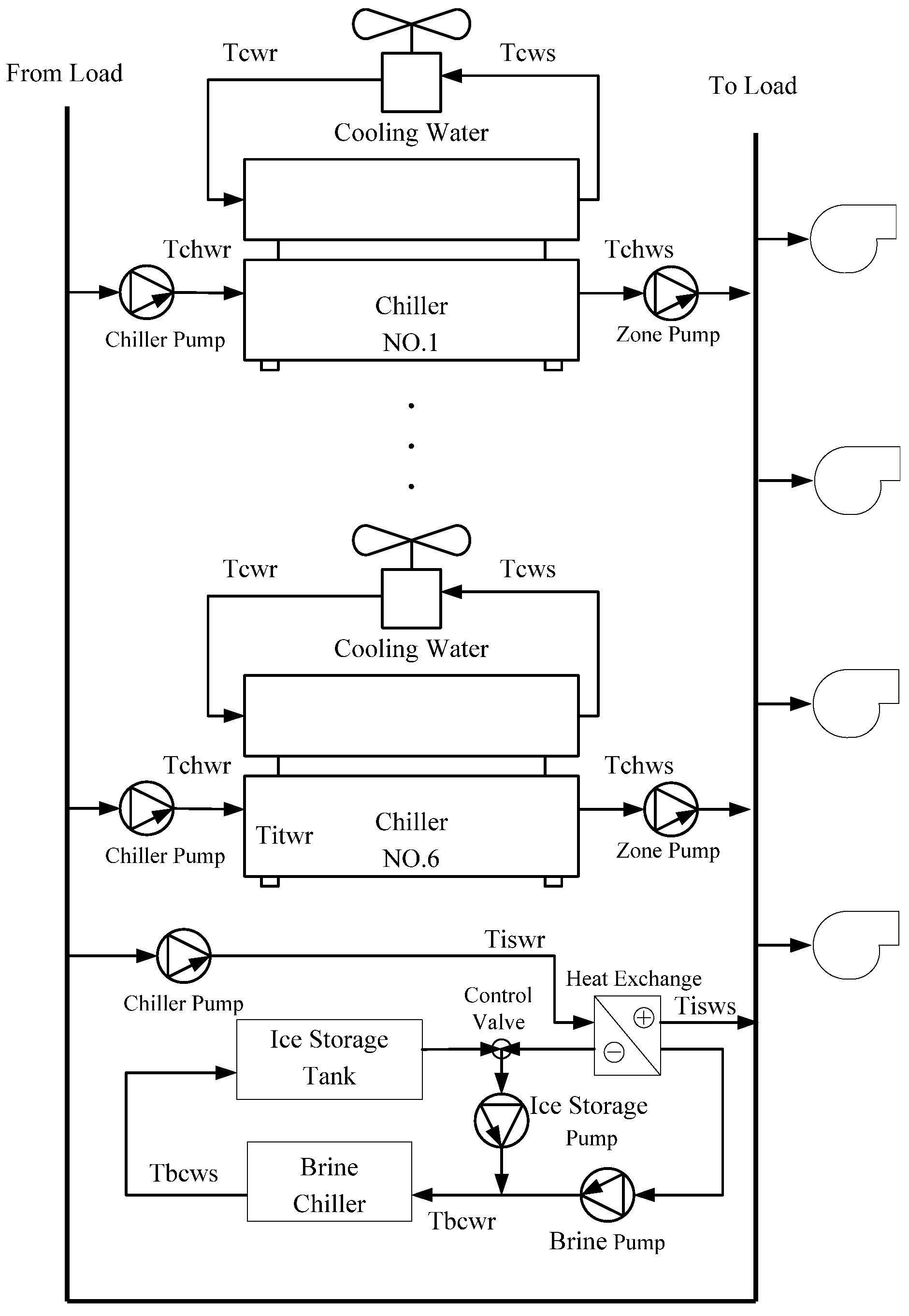
2.1. The Cooling Load Capacity of Chillers

The cooling load capacity for chillers is generally calculated based on the return water temperature, supply water temperature, and the flow rate of chilled water. Therefore, the calculation of the cooling load capacity for the chillers is as in Equation (1):

$$Q_{chiller}=LP{M}_{chiller}\times \text{Δ}{T}_{chw}\times {\rho }_w\times C_{p,chiller}$$

(1)

• $Q_{chiller}$: the cooling load of chillers (kJ/hr);
• $LP{M}_{chiller}$: the flow rate of chilled water (liter/hr);
• ${\rho }_w$: the density of chilled water (1 kg/L);
• $C_{p,chiller}$: the specific heat of water at average temperature (4.186kJ/kg-°C).
• $\text{Δ}{T}_{chw}$ is the temperature difference of chilled water (°C), which is defined as Equation (2):

  $$\text{Δ}{T}_{chw}=T_{chwrt}-T_{chwst}$$

  (2)
• $T_{chwrt}$: the return temperature of chilled water (°C);
• $T_{chwst}$: the supply temperature of chilled water (°C).

2.2. The Cooling Load Capacity of the Ice Storage Tank

The cooling load capacity of the ice storage tank is calculated based on the return water temperature, supply water temperature, and the flow rate of chilled water. Therefore, the calculation of the cooling load capacity is represented as in Equation (3):

$$Q_{ice}=\text{Δ}{T}_{isw}\times LP{M}_{ice}\times C_{p,ice}$$

(3)

$$\text{Δ}{T}_{isw}=T_{iswr}-T_{isws}$$

(4)

• $\text{Δ}{T}_{isw}$: the temperature difference of ice storage brine (°C);
• $C_{p,ice}$: the specific heat of ice storage brine at average temperature (3.6 kJ/kg-°C);
• $T_{iswr}$: the return temperature of ice storage brine (°C);
• $T_{isws}$: the supply temperature of ice storage brine (°C);
• $LP{M}_{ice}$: the flow rate of ice storage brine (L/h);
• $Q_{ice}$: cooling load capacity of the ice storage tank (kJ/h).

2.3. Power Consumption of Cooling Towers and Pumps

The power consumption of the cooling tower ($P_{tower}$) is calculated from the fan motor. The power consumption of cooling tower is regarded as proportional to the cooling tower capacity ($t_{wrld}$). It can be computed as in Equations (5) and (6) [29]:

$$t_{wrld,i}=P_{chiller,i}+Q_{chille,i}\times (3.517kW/ton)$$

(5)

$$P_{tower,i}=0.025\times t_{wrld,i}$$

(6)

The consumption power of pump ($P_{pump}$)is calculated with the total chilled water-mass flow rate($G_p$), head loss($\text{Δ}H$), and pump efficiency(${\eta }_p$) as in Equation (7) [29]:

$$P_{\text{pump}}=\frac{G_p\times \text{Δ}H}{3960\times {\eta }_p}$$

(7)

2.4. Power Consumption of Chillers and Ice Storage Tanks

The power consumption of chillers is a convex function of the cooling load capacity as shown in Equation (8):

$$P_{chiller,i}=a_i+b_i{Q}_{chiller,i}+c_i{Q}_{chiller,i}^2+d_i{Q}_{chiller,i}^3$$

(8)

where $a_i$, $b_i$, $c_i$, and $d_i$ are the regression coefficients of the function of cooling load capacity and power consumption.

The power consumption of the ice storage tank is also a convex function of the cooling load capacity as shown in Equation (9):

$$P_{ice,i}=a_{ice,i}+b_{ice,i}{Q}_{ice,i}+c_{ice,i}{Q}_{ice,i}^2+d_{ice,i}{Q}_{ice,i}^3$$

(9)

where $a_{ice,i}$, $b_{ice,i}$, $c_{ice,i}$, and $d_{ice,i}$ are regression coefficients of the function of $P_{ice,i}$.

2.5. Objective Function and Constraints

The main purpose of this paper is to derive the best single-day schedule planning for ice storage air-conditioning systems so that the total cooling load of the chillers and ice storage tank can meet the required cooling needs of the target space. The total electricity cost is also minimized as in Equation (10):

$$Min\text{. }Cost={\displaystyle \sum _{t=1}^H\left[\begin{array}{l}\left({\displaystyle \sum _{i=1}^L{P}_{chiller,i}(t)}{U}_i(t)+{\displaystyle \sum _{i=1}^N{P}_{tower,i}(t)}+P_{pump}(t)\right)\times EC(t)\\ +{\displaystyle \sum _{i=1}^M{P}_{ice,i}(t)}\times U_i(t)\times EC(t)\end{array}\right]}$$

(10)

• $P_{chiller,i}(t)$: the power consumption of the i-th chiller at time t;
• $P_{tower,i}(t)$: the power consumption of the i-th cooling tower at time t;
• $P_{pump}(t)$: the power consumption of pump at time t;
• $U_i(t)$: the i-th unit on/off at time t, 1 is on and 0 is off;
• $EC(t)$: the TOU rates as shown in Figure 2 [26];
• $P_{ice}(t)$: power consumption of the ice storage at time t (kW);
• $H$: the scheduling time;
• $L$: the total number of chillers;
• $M$: the total number of ice storage tanks.

Figure 2. The TOU rate for a summer day and a non-summer day.

Figure 2. The TOU rate for a summer day and a non-summer day.

The constraints include both the system constraints and the unit’s constraints:

(a) load balance:

$$\left({\displaystyle \sum _{i=1}^L{Q}_{chiller,i}(t)}{U}_i(t)+{\displaystyle \sum _{i=1}^M{Q}_{ice,i}(t)U_i(t)}\right)\ge CL(t)$$

(11)

(b) the limitation for the temperature difference of chilled water:

$$\text{Δ}{T}_{chw,\min }^i\le \text{Δ}{T}_{chw}^i(t)\le \text{Δ}{T}_{chw,amx}^i$$

(12)

(c) the limitation for the temperature difference of the ice storage tank:

$$\text{Δ}{T}_{isw,\min }^i\le \text{Δ}{T}_{isw}^i(t)\le \text{Δ}{T}_{isw,amx}^i$$

(13)

where $Q_{chiller,i}(t)$ is the cooling load of the i-th chiller at time t (kJ/hr), $Q_{ice}(t)$ is the cooling load of the i-th ice storage at time t (kJ/hr) and $CL(t)$ is the total system cooling load at time t (kJ/hr). $\text{Δ}{T}_{chw}^i(t)$ is the temperature difference of the i-th chilled water at t-th time. $\text{Δ}{T}_{chw,\max }^i$ and $\text{Δ}{T}_{chw,\min }^i$ are the maximum and minimum generation limits of the temperature difference of the i-th chilled water. $\text{Δ}{T}_{isw}^i(t)$ is the temperature difference of the i-th ice storage tank at time t. $\text{Δ}{T}_{isw,\max }^i$ and $\text{Δ}{T}_{isw,\min }^i$ are the maximum and minimum generation limits of the temperature difference of the i-th ice storage tank.

3. The Proposed Methodology

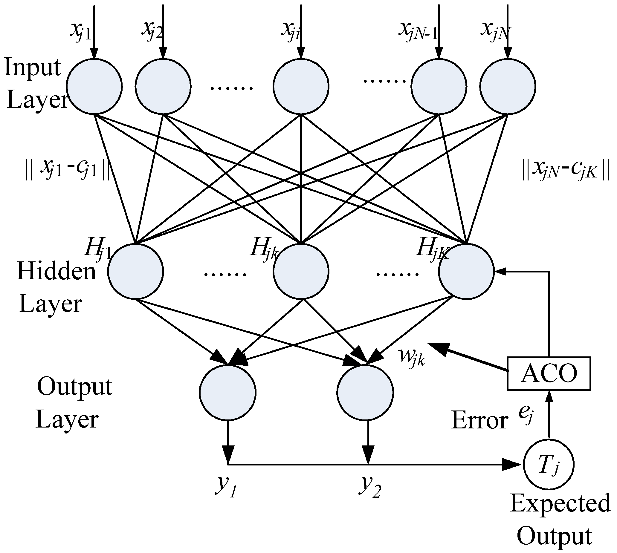
ARBFN consists of the input, hidden, and output layers. The unknown j-th input vector X_j=[x_j1, x_j2, …, x_ji, …, x_jN], i = 1, 2,…, N, j = 1, 2,…, M, is connected to the input layer. The number of output nodes y_j, j = 1, 2,…, M, is equal to the number of training input-output data pairs, that is to say, input nodes (a matrix) and output nodes (a vector) are paired. The j-th hidden nodes vector H_j=[H_j1, H_j2, …, H_jk, …, H_jK], k = 1, 2, …, K, j = 1, 2, …, M. The weights w_jk connect the k-th hidden node with the j-th output node. The ARBFN structure is shown in Figure 3, and the “ACO” process is performed in the adjusting error stage.

Figure 3. The ARBFN Structure j-th forecast.

Figure 3. The ARBFN Structure j-th forecast.

3.1. Input Layer

In this paper, x_i is the i-th variable of the expected output. For each training data pair, set input matrix X = [x_ji] _M×N, j=1, 2, …, M, i = 1, 2, …, N.

3.2. Hidden Layer

In the hidden layer, C_j=[c_j1, …, c_jk, …, c_jK] is called the j-th center of EACO. ║x_ji −c_jk║ is the Euclidean distance between the i-th node of the input layer and the k-th node of the hidden layer. The Euclidean distance is determined by Equation (14):

$$||x_{ji}-c_{jk}||=\sqrt{{\displaystyle \sum _{i=1}^N{(x_{ji}-c_{jk})}^2}}$$

(14)

The k-th hidden layer output is defined as Equation (15):

$$H_{jk}={\phi }_{jk}(\sqrt{{\displaystyle \sum _{i=1}^N{(x_{ji}-c_{jk})}^2}})$$

(15)

In Equation (16), the function φ(•) is a Gaussian distribution function and σ is a smoothing parameter:

$$\phi (x)=e^{-x^2/{\sigma }^2}$$

(16)

3.3. Output Layer

In the output layer, let w_jk be the weight between hidden node H_jk and output node y_j, and the j-th output of the output layer is given as Equation (17):

$$y_j={\displaystyle \sum _{k=1}^K{w}_{jk}{H}_{jk}}$$

(17)

In order to adjust the three parameters, which are weights w_jk, the center of C and the smoothing parameters σ_jk of function φ(•), ACO is adopted. The ACO process is:

1)

Calculate Euclidean distance ║x_ji ﹣c_jk║;

2)

Calculate hidden layer output H_jk by Equation (15);

3)

Calculate output layer output by Equation (17);

4)

Calculate the error between simulation output y_j and its expected value T_j by error function. In this paper, the fitness function is set to an error function which is defined as Equation (18):

$$\begin{array}{l}{e}_j(n)={\left[T_j-y_j(n)\right]}^2\\ ={\left[T_j-{\displaystyle \sum _{k=1}^K{w}_{jk}(n)exp\left(-\frac{{\Vert X_j(n)-C_{jk}(n)\Vert }^2}{{\sigma }_{jk}^2(n)}\right)}\right]}^2\end{array}$$

(18)

where e_j(n) and y_j(n) is the j-th error and the j-th simulation output of the n-th epoch, respectively. The related parameters are updated by Equations (19)–(21):

$$w_{jk}(n+1)=w_{jk(n)}-{\mu }_{jw}\frac{\partial }{\partial w_{jk}}{e}_j(n)$$

(19)

$$c_{jk}(n+1)=c_{jk(n)}-{\mu }_{jc}\frac{\partial }{\partial c_{jk}}{e}_j(n)$$

(20)

$${\sigma }_{jk}(n+1)={\sigma }_{jk(n)}-{\mu }_{j\sigma }\frac{\partial }{\partial {\sigma }_{jk}}{e}_j(n)$$

(21)

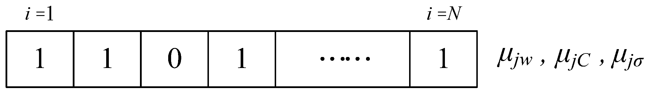
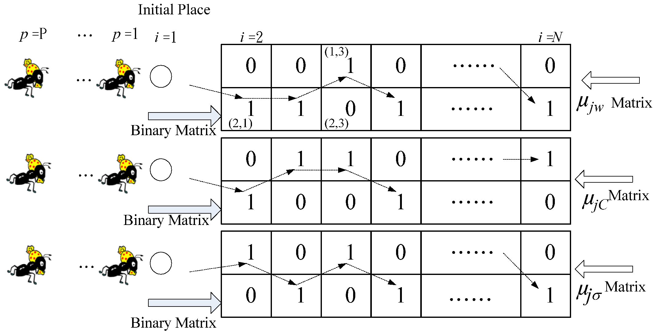
3.4. Ant Colony Optimization (ACO) Process

The ACO optimization method is used to optimize three learning rate parameters ${\mu }_{iw}$, ${\mu }_{ic}$, and ${\mu }_{i\sigma }$. These optimal parameters refine the accuracy in a dynamic environment and can yield a minimum forecast error based on the testing data. The ACO process as applied to the learning rate parameters is as follows:

Step 1: Set $P$ ants, pheromone intensity ${\tau }_{ij}$, and consciousness constant ${\eta }_{ij}$ for each learning rate parameter.

Step 2: In the learning process of ARBFN, the ants deposit their own pheromones along the path, and exploration denotes the process of selecting a path by probability. The initial solution is obtained by assigning a binary digit for the learning rate parameters as shown in Figure 4. To avoid an ant repeatedly visiting the same place, each ant $p$ has its own path at time $i$ to memorize where the ant has gone. ${\tau }_{ij}$ and ${\eta }_{ij}$ are used to control the ant’s direction of movement to another place.

Figure 4. A binary digit for the learning rate parameters.

Figure 4. A binary digit for the learning rate parameters.

In this paper, an ant matrix is designed to represent an ant’s paths ($tab{u}^p(i)$). In order to deposit two statuses along the path, an ant’s path matrix ($tab{u}^p(i)$) is defined as in Figure 5. The process of the learning rate parameters operates as ants travel selecting paths, and evaluated by the fitness values of all ants until a specified training accuracy is attained. A sample is used to describe the basic concept of the ant matrix, shown in Figure 5. If an ant of parameter ${\mu }_{jw}$ is located at array (2,1) after the fitness value is calculated, the binary digit is set to 1 because the fitness value at array (2,1) is best along this stage. The binary digit of array (1,1) will then be set to 0. When the ant passes array (1,3), the binary digit of array (2,3) will be set to 0. Simultaneously, the ants of parameters ${\mu }_{jc}$ and ${\mu }_{j\sigma }$ will conduct their paths. A new path matrix is generated when the ants have completely explored the path.

Figure 5. The basic concept of the ant matrix.

Figure 5. The basic concept of the ant matrix.

Step 3: Calculate the probability of the ants’ path.

The state transition rule of the ant path matrix used by ACO is given by Equation (22), which gives the probability of ant $p$ being at array $(i,j)$:

$$P_{ij}^p(t)=\{\begin{array}{c}\frac{\alpha \cdot {\tau }_{ij}^p(t)+(1-\alpha )\cdot {\eta }_{ij}^p}{{\displaystyle \sum _{l\notin {\text{tabu}}^p}\text{(}\alpha \cdot {\tau }_{il}^p(t)+(1-\alpha )\cdot {\eta }_{ij}^p}},j\notin {\text{tabu}}^p\\ 0,otherwise\end{array}$$

(22)

where $0<\alpha <\text{1}$ is a pheromone decay parameter, ${\tau }_{ij}^p(t)$ is the pheromone intensity at time $t$ and ${\eta }_{ij}^p(t)$ is the pheromone consciousness at time t.

Step 4: Generate the new binary matrix and calculate the learning for ${\mu }_{jw}(t+1)$, ${\mu }_{jc}(t+1)$, and ${\mu }_{j\sigma }(t+1)$.

Step 5: Calculate the output error of the fitness function.

Step 6: Update the pheromone intensity:

$${\tau }_{ij}^p(t+1)=\rho {\tau }_{ij}^p(t)+\Delta {\tau }_{ij}^p$$

(23)

where $\rho$ is the pheromone intensity constant ($0\le \rho \le 1$), and $\Delta {\tau }_{ij}^p$ is the deviation of pheromone intensity as shown in Equation (24):

$$\text{Δ}{\tau }_{ij}^p=\{\begin{array}{c}Q/e_{ij}^p,thepath(i,j)forp-thant\\ 0,other\end{array}$$

(24)

where Q is the pheromone release rate ($0\le Q\le 1$), and $e_{ij}^p$ is the error of path (i,j) for the p-th ant.

Step 7: Stopping Rule.

A fitness function error of 0.00001 is set as the stopping criterion. If the convergent condition is not met, Steps 2 to 6 will be repeated.

3.5. Implementation of ARBFN

Power consumption fluctuations may be the result of temperature ($Temp$), Partial Load Regulation ($PLR$), $LP{M}_{chiller}$, $LP{M}_{ice}$, the percent of ice stored tank($ICE$), or the temperature difference in an ice storage air-conditioning system. ARBFN is capable of coping with complicated interactions among these factors. These factors can, thus, be taken into account as inputs to the ARBFN.

The operating data for chillers and ice storage tanks are collected and divided into input variables and output variables. In this study, three ARBFNs are trained in the 24 h schedule. ARBFN training is conducted to minimize the fitting error for a sample training set. The output layer contains two output variables: power consumption and cooling load. The hidden layer contains K hidden nodes. The variables of the input layer depend on the types of units. Three training nets are proposed in this study.

(1) Chiller nets:

$$input=\left[Temp,T_{chwrt},LP{M}_{chiller},PLR,\hspace{0.17em}\text{Δ}{T}_{chw}\right]$$

(25)

$$output=\left[P_{chiller},Q_{chiller}\right]$$

(26)

(2) Ice storage tank in charging process:

$$input=\left[Temp,\hspace{0.17em}\text{Δ}{T}_{bcw},\hspace{0.17em}\text{Δ}{T}_{bccw},LP{M}_{ice},ICE\right]$$

(27)

$$output=\left[P_{ice},Q_{ice}\right]$$

(28)

where $\text{Δ}{T}_{bcw}$ is temperature difference of brine for ice-storage tank (°C), $\text{Δ}{T}_{bccw}$ is temperature difference of brine for the cooling pump (°C). The sample data from the ice storage air-conditioning system in Chang-Cung Memorial Hospital were collected and constructed in EXCEL Workspace. The data analysis and data storage can be easily manipulated with this database. The ARBFN consists of the input, hidden and output layers. The learning rates ${\mu }_w,{\mu }_c,{\mu }_{\sigma }$ were adjusted by ACO as shown in Figure 3. The ACO technique finds the optimal solution using a population of ants. The population size is set to $P=20$ and the dimension is set to $d=3$. The ant generations are ${\mu }_i^d=[{\mu }_w,{\mu }_c,{\mu }_{\sigma }]$, where ${\mu }_w$, ${\mu }_c$, and ${\mu }_{\sigma }$ are the ARBFN learning rates.

4. Case Study

The proposed algorithm was tested in a real ice storage air-conditioning system, which include six chillers and one ice storage tank. The cooling capability of the chillers have two sets of 550RT chillers (NO1 and NO2) and four sets of 1000RT chillers (NO3–NO6). The cooling capability of the ice storage tank has 8000RT (NO7). The cooling capability for each RT is 13910 KJ/hr. The real ice storage air-conditioning system is currently operated in a ON/OFF status depend on day or night. The electricity cost for the chillers and ice storage tank was calculated based on the announced summer and non-summer prices from the Taiwan Power Company (TPC) as shown in Figure 2. By using the measurement data, the LSR was used to get the I/O operation curves of the chillers and the ice storage tank. Table 1 shows the coefficients of the I/O operation curve for the chillers and the ice storage tank. The rated limits for the ice storage air-conditioning system are given in Table 2.

Table 1. The coefficients of the I/O operation curve for chillers and ice storage tank.

Unit	a	b	c	d
$P_{chiller,1}$	65.7772	0.1961	1.3707E-08	1.249E-09
$P_{chiller,2}$	128.7969	0.0449	1.139E-04	−2.628E-08
$P_{chiller,3}$	68.2033	0.1418	4.13921E-05	−7.599E-09
$P_{chiller,4}$	107.7250	0.1181	1.87115E-05	−1.467E-09
$P_{chiller,5}$	623.2087	−0.4555	0.000228205	−2.660E-08
$P_{chiller,6}$	101.5365	0.0851	6.87455E-05	−1.141E-08
Charging Process Pice	2204.5246	−24.3534	9.252E-02	−1.022E-04
Discharging Process Pice	−21.7173	0.2206	5.533E-05	−1.591E-08

Table 1. The coefficients of the I/O operation curve for chillers and ice storage tank.

Unit	a	b	c	d
$P_{chiller,1}$	65.7772	0.1961	1.3707E-08	1.249E-09
$P_{chiller,2}$	128.7969	0.0449	1.139E-04	−2.628E-08
$P_{chiller,3}$	68.2033	0.1418	4.13921E-05	−7.599E-09
$P_{chiller,4}$	107.7250	0.1181	1.87115E-05	−1.467E-09
$P_{chiller,5}$	623.2087	−0.4555	0.000228205	−2.660E-08
$P_{chiller,6}$	101.5365	0.0851	6.87455E-05	−1.141E-08
Charging Process Pice	2204.5246	−24.3534	9.252E-02	−1.022E-04
Discharging Process Pice	−21.7173	0.2206	5.533E-05	−1.591E-08

Table 2. The operational parameter limits.

Chiller NO1	Max.	Min.	Chiller NO2	Max.	Min.
PLR(%)	100	50	PLR(%)	100	50
$\text{Δ}{T}_{chw}$	5	2.5	$\text{Δ}{T}_{chw}$	5	2.5
$\text{Δ}{T}_{cw}$	5	3	$\text{Δ}{T}_{cw}$	5	3
Chiller NO3	Max.	Min.	Chiller NO4	Max.	Min.
PLR(%)	100	50	PLR(%)	100	50
$\text{Δ}{T}_{chw}$	5	2.5	$\text{Δ}{T}_{chw}$	5	2.5
$\text{Δ}{T}_{cw}$	5	2	$\text{Δ}{T}_{cw}$	5	3.5
Chiller NO5	Max.	Min.	Chiller NO6	Max.	Min.
PLR(%)	100	50	PLR(%)	100	50
$\text{Δ}{T}_{chw}$	5	2.5	$\text{Δ}{T}_{chw}$	5	2.5
$\text{Δ}{T}_{cw}$	5	3.5	$\text{Δ}{T}_{cw}$	5	2
Charge Process	Max.	Min.	Discharge Process	Max.	Min.
$\text{Δ}{T}_{bcw}$	3.9	1.9	$\text{Δ}{T}_{isw}$	11	5.6
$\text{Δ}{T}_{bccw}$	4.2	2.6	Control Valve(LPM)	5109.1	3627

Table 2. The operational parameter limits.

Chiller NO1	Max.	Min.	Chiller NO2	Max.	Min.
PLR(%)	100	50	PLR(%)	100	50
$\text{Δ}{T}_{chw}$	5	2.5	$\text{Δ}{T}_{chw}$	5	2.5
$\text{Δ}{T}_{cw}$	5	3	$\text{Δ}{T}_{cw}$	5	3
Chiller NO3	Max.	Min.	Chiller NO4	Max.	Min.
PLR(%)	100	50	PLR(%)	100	50
$\text{Δ}{T}_{chw}$	5	2.5	$\text{Δ}{T}_{chw}$	5	2.5
$\text{Δ}{T}_{cw}$	5	2	$\text{Δ}{T}_{cw}$	5	3.5
Chiller NO5	Max.	Min.	Chiller NO6	Max.	Min.
PLR(%)	100	50	PLR(%)	100	50
$\text{Δ}{T}_{chw}$	5	2.5	$\text{Δ}{T}_{chw}$	5	2.5
$\text{Δ}{T}_{cw}$	5	3.5	$\text{Δ}{T}_{cw}$	5	2
Charge Process	Max.	Min.	Discharge Process	Max.	Min.
$\text{Δ}{T}_{bcw}$	3.9	1.9	$\text{Δ}{T}_{isw}$	11	5.6
$\text{Δ}{T}_{bccw}$	4.2	2.6	Control Valve(LPM)	5109.1	3627

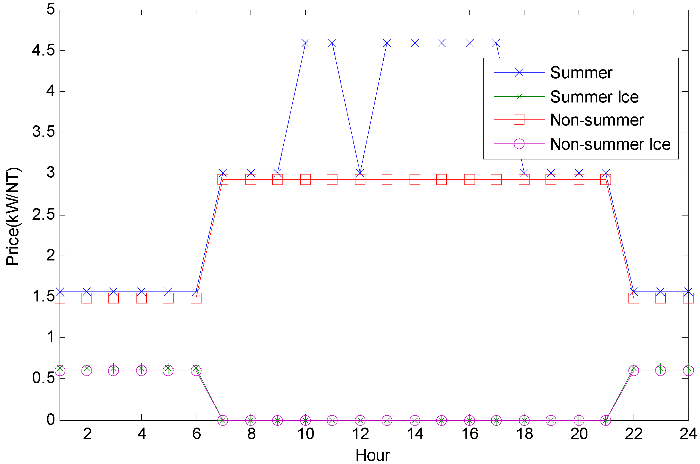
4.1. Results at Different TOU Intervals

ARBFN was used to test the functions of six sets of chillers and the ice storage tank, and the condition parameters on 17 July 2013 (summer day) and 21 October 2013 (non-summer day) were simulated. The hourly required cooling capacity, outside air temperature and $T_{chwrt}$ of the ice storage system were collected from 22:00 of the previous days, 16 July 2013 and 20 October 2013, until 21:00 of the following days, 17 July 2013 and 21 October 2013.

Table 3 shows the energy dispatch results of ice storage air-conditioning systems during a total scheduling of 24 h periods on the summer day. From Table 3, during off-peak hours when the cooling load is smaller, the ice maker stores the required cooling energy in the storage tank. During the peak hours, the storage tank provides the required cooling load. Furthermore, although the power consumption during peak hours is lower, the cost will be greater. It can also be shown that the TOU rate will influence the overall economy of the ice storage air-conditioning system.

Table 3. Energy dispatch results on summer day (17 July 2013).

Hour	Chiller						ICE (%)	Power (kW)	Cost (NT$)
	NO1	NO2	NO3	NO4	NO5	NO6
22	1	1	1	0	1	1	7.10	3152.97	4620.07
23	1	1	0	1	1	1	14.64	3144.25	4593.52
24	0	0	1	1	1	1	22.78	3037.77	4409.24
1	0	1	1	1	1	1	31.42	3013.29	4353.75
2	1	1	1	0	1	1	40.64	3087.55	4452.04
3	1	1	1	1	1	0	49.18	3062.86	4424.93
4	0	1	1	1	1	0	58.17	2760.67	3948.25
5	0	1	0	1	1	1	65.85	2667.75	3836.68
6	0	1	1	0	1	1	73.39	2583.26	3716.21
7	0	0	1	1	1	0	65.87	1758.33	5292.58
8	0	0	1	1	1	1	60.12	2532.70	7623.44
9	0	0	0	1	1	1	51.25	2203.22	6631.69
10	0	0	1	1	1	1	44.73	2507.66	11510.18
11	1	1	1	0	1	1	37.33	2625.41	12050.61
12	1	0	1	1	1	0	27.98	2379.28	7161.63
13	0	1	1	1	1	1	20.87	2702.69	12405.37
14	1	0	1	1	1	0	11.50	2445.28	11223.84
15	1	0	1	1	1	1	1.94	2589.96	11887.91
16	1	0	1	1	1	1	0.00	2792.89	12819.35
17	1	0	1	1	1	1	0.00	3143.81	14430.08
18	0	1	1	1	1	1	0.00	3163.51	9522.18
19	0	1	1	1	1	1	0.00	3027.51	9112.82
20	1	1	1	1	0	1	0.00	2878.31	8663.70
21	0	0	1	1	1	1	0.00	2655.52	7993.12
Total								65916.46	186683.17

Table 3. Energy dispatch results on summer day (17 July 2013).

Hour	Chiller						ICE (%)	Power (kW)	Cost (NT$)
	NO1	NO2	NO3	NO4	NO5	NO6
22	1	1	1	0	1	1	7.10	3152.97	4620.07
23	1	1	0	1	1	1	14.64	3144.25	4593.52
24	0	0	1	1	1	1	22.78	3037.77	4409.24
1	0	1	1	1	1	1	31.42	3013.29	4353.75
2	1	1	1	0	1	1	40.64	3087.55	4452.04
3	1	1	1	1	1	0	49.18	3062.86	4424.93
4	0	1	1	1	1	0	58.17	2760.67	3948.25
5	0	1	0	1	1	1	65.85	2667.75	3836.68
6	0	1	1	0	1	1	73.39	2583.26	3716.21
7	0	0	1	1	1	0	65.87	1758.33	5292.58
8	0	0	1	1	1	1	60.12	2532.70	7623.44
9	0	0	0	1	1	1	51.25	2203.22	6631.69
10	0	0	1	1	1	1	44.73	2507.66	11510.18
11	1	1	1	0	1	1	37.33	2625.41	12050.61
12	1	0	1	1	1	0	27.98	2379.28	7161.63
13	0	1	1	1	1	1	20.87	2702.69	12405.37
14	1	0	1	1	1	0	11.50	2445.28	11223.84
15	1	0	1	1	1	1	1.94	2589.96	11887.91
16	1	0	1	1	1	1	0.00	2792.89	12819.35
17	1	0	1	1	1	1	0.00	3143.81	14430.08
18	0	1	1	1	1	1	0.00	3163.51	9522.18
19	0	1	1	1	1	1	0.00	3027.51	9112.82
20	1	1	1	1	0	1	0.00	2878.31	8663.70
21	0	0	1	1	1	1	0.00	2655.52	7993.12
Total								65916.46	186683.17

Figure 6 shows the cooling capability provided by each chiller and the ice storage tank on a summer day. From Figure 6, the ice storage tank supplies the required cooling load during peak periods. All chillers are appropriately dispatched to achieve minimal cost.

Figure 6. Cooling capability provided by each chiller and the ice storage tank on a summer day (17 July 2013).

Figure 6. Cooling capability provided by each chiller and the ice storage tank on a summer day (17 July 2013).

Table 4 shows the energy dispatch results of ice storage air-conditioning systems during a total scheduling of 24 h periods on a non-summer day. Similarly, although the power consumption is lower during peak periods, the cost is still greater. This shows that the TOU rate plays an important role in this study.

Table 4. Energy planning for ice storage air conditioning on non-summer day (21 October 2013).

Hour	Chiller						ICE (%)	Power (kW)	Cost (NT$)
	NO1	NO2	NO3	NO4	NO5	NO6
22	0	1	0	1	1	1	7.69	1885.10	2466.67
23	1	1	1	1	0	1	16.96	2139.77	2810.98
24	0	1	1	1	1	1	25.43	2098.53	2766.18
1	0	1	0	1	1	1	34.68	2103.68	2758.08
2	1	0	0	1	0	1	43.67	2042.69	2674.30
3	1	0	1	1	0	1	52.65	2057.44	2699.09
4	1	1	0	1	1	1	59.48	1995.04	2652.43
5	1	1	0	1	0	1	68.17	2015.33	2650.33
6	1	0	1	1	1	0	75.66	1895.39	2499.20
7	1	0	0	0	0	1	68.49	958.99	2809.83
8	0	0	1	0	1	1	63.45	1543.89	4523.59
9	0	1	1	1	0	1	56.55	1551.37	4545.51
10	0	0	1	1	1	0	51.93	1679.36	4920.53
11	0	0	1	1	1	0	44.31	1432.15	4196.20
12	0	1	1	1	1	0	38.00	1717.87	5033.35
13	0	0	0	1	1	1	32.19	1645.15	4820.30
14	0	1	1	0	1	0	24.92	1541.14	4515.53
15	0	0	1	1	1	0	19.39	1496.22	4383.93
16	0	0	1	1	1	0	14.88	1416.48	4150.27
17	1	0	1	0	0	1	10.52	1363.52	3995.11
18	0	0	1	1	0	0	7.12	1236.36	3622.52
19	0	0	1	1	1	0	5.66	1273.19	3730.45
20	0	0	1	0	0	1	1.96	926.44	2714.47
21	0	0	0	1	1	0	0.00	944.50	2767.38
Total								38959.58	84706.24

Table 4. Energy planning for ice storage air conditioning on non-summer day (21 October 2013).

Hour	Chiller						ICE (%)	Power (kW)	Cost (NT$)
	NO1	NO2	NO3	NO4	NO5	NO6
22	0	1	0	1	1	1	7.69	1885.10	2466.67
23	1	1	1	1	0	1	16.96	2139.77	2810.98
24	0	1	1	1	1	1	25.43	2098.53	2766.18
1	0	1	0	1	1	1	34.68	2103.68	2758.08
2	1	0	0	1	0	1	43.67	2042.69	2674.30
3	1	0	1	1	0	1	52.65	2057.44	2699.09
4	1	1	0	1	1	1	59.48	1995.04	2652.43
5	1	1	0	1	0	1	68.17	2015.33	2650.33
6	1	0	1	1	1	0	75.66	1895.39	2499.20
7	1	0	0	0	0	1	68.49	958.99	2809.83
8	0	0	1	0	1	1	63.45	1543.89	4523.59
9	0	1	1	1	0	1	56.55	1551.37	4545.51
10	0	0	1	1	1	0	51.93	1679.36	4920.53
11	0	0	1	1	1	0	44.31	1432.15	4196.20
12	0	1	1	1	1	0	38.00	1717.87	5033.35
13	0	0	0	1	1	1	32.19	1645.15	4820.30
14	0	1	1	0	1	0	24.92	1541.14	4515.53
15	0	0	1	1	1	0	19.39	1496.22	4383.93
16	0	0	1	1	1	0	14.88	1416.48	4150.27
17	1	0	1	0	0	1	10.52	1363.52	3995.11
18	0	0	1	1	0	0	7.12	1236.36	3622.52
19	0	0	1	1	1	0	5.66	1273.19	3730.45
20	0	0	1	0	0	1	1.96	926.44	2714.47
21	0	0	0	1	1	0	0.00	944.50	2767.38
Total								38959.58	84706.24

Figure 7 shows the cooling capability provided by each chiller and the ice storage tank on a non-summer day. From Figure 7, the ice storage tank also supplies the required cooling load during peak periods. All chillers are also appropriately dispatched to achieve minimal cost.

Figure 7. Cooling capability provided by each chiller and the ice storage tank on 21 October 2013.

Figure 7. Cooling capability provided by each chiller and the ice storage tank on 21 October 2013.

4.2. Energy Reduction Analysis

Table 5 shows the actual power consumption measured for an ice storage air-conditioning system and the actual energy consumption analysis of ARBFN and LSR. In Table 5, the “actual” data, which is the power consumption of a daily schedule, are the actual measurements of the ice storage air-conditioning system. The estimations of the ARBFN and LSR were compared as shown in Table 5. The power consumption reduction error of ARBFN on summer day is 1.34% and on non-summer day is 0.68%, while the errors of LSR are 6.68% and 5.74%, respectively. Therefore, the accuracy of the ARBFN models can be verified. If LSR is chosen for scheduling assessment of the ice-storage air-conditioning system, larger errors on costs tend to occur.

Table 5. The energy reduction analysis of ARBFN and LSR.

		Actual	ARBFN	Difference	Reduction (%)	LSR	Difference *	Reduction (%)
Summer day	Power consumption (KW)	68,481.8	67,562.4	1232	1.34	73,054.8	30,548	6.68
	Total cost (NT$)	194,726	192,310	2996	1.24	181,517	89,557	6.78
Non-summer day	Power Consumption (KW)	41,456.9	41,739.9	192	0.68	39,079.1	13,648	5.74
	Total cost (NT$)	91,457	92,249	689	0.87	98,605	51,823	7.25

* Difference = Actual – ARBFN × $Reduction(\%)=\frac{\left|Actual-ARBFN\right|}{Actual}\times 100\%$.

Table 5. The energy reduction analysis of ARBFN and LSR.

		Actual	ARBFN	Difference	Reduction (%)	LSR	Difference *	Reduction (%)
Summer day	Power consumption (KW)	68,481.8	67,562.4	1232	1.34	73,054.8	30,548	6.68
	Total cost (NT$)	194,726	192,310	2996	1.24	181,517	89,557	6.78
Non-summer day	Power Consumption (KW)	41,456.9	41,739.9	192	0.68	39,079.1	13,648	5.74
	Total cost (NT$)	91,457	92,249	689	0.87	98,605	51,823	7.25

* Difference = Actual – ARBFN × $Reduction(\%)=\frac{\left|Actual-ARBFN\right|}{Actual}\times 100\%$.

4.3. Convergence Test

Table 6 shows the comparisons of ARBFN, GA with RBFN (GA-RBFN), and EP with RBFN (EP-RBFN) in a daily schedule. An IBM PC with a P-IV 2.0 GHz CPU and 512 MB SDRAM was used for this test. The improvement of the ARBFN over other algorithms is clear. The average execution times for ARBFN, GA-RBFN, and EP-RBFN were only 5.67 s, 4.81 s, and 3.54 s, respectively. Although the executed performance of ARBFN was subtle, it did show the capacity of ARBFN to explore a more likely global optimum. From Table 6, it is clear that the operating plans of the chillers and ice storage tank save 2565.33 (kW) of electricity consumption and 5626.83 (NT$) in electricity costs in summer. On non-summer day, the savings on power consumption are 2780.32 (kW) and 7542.8 (NT$). The electricity savings on a summer day and on a non-summer day are 2.89% and 8.25%, respectively. It can be shown that the proposed algorithm can also yield a better plan for ice storage and melting procedures.

Table 6. Comparison of ARBFN, GA with RBFN, and EP with RBFN.

Algorithms	Summer Day		Non-Summer Day
	Power consumption (KW)	Total Cost (NT$)	Power Consumption (KW)	Total Cost (NT$)
ARBFN	65,916.46	186,683.17	38,959.58	84,706.24
GA-RBFN	66,148.61	187,309.84	39,287.41	85,371.62
EP-RBFN	66,431.83	188,131.15	39,514.37	85,984.38

Table 6. Comparison of ARBFN, GA with RBFN, and EP with RBFN.

Algorithms	Summer Day		Non-Summer Day
	Power consumption (KW)	Total Cost (NT$)	Power Consumption (KW)	Total Cost (NT$)
ARBFN	65,916.46	186,683.17	38,959.58	84,706.24
GA-RBFN	66,148.61	187,309.84	39,287.41	85,371.62
EP-RBFN	66,431.83	188,131.15	39,514.37	85,984.38

5. Conclusions

This paper proposed ARBFN to solve the ice storage air-conditioning system dispatch problem so as to reduce buildings’ electricity expenses. The data, including the operational data of chillers, the ice-storage tank charging process, and ice-storage tank discharging process in the field, were calculated, and the data clusters were embedded in an Excel database. Based on the TOU and all technical constraints, the dispatch model of the ice storage air-conditioning system was formulated by considering the charging/discharging scheduling of ice storage systems. A real case was used to verify the effectiveness of the proposed method. Simulation results provide a practical and flexible framework for operators to perform the economic dispatch of the ice storage air-conditioning system. This can also provide greater energy efficiency in dispatching chillers, thus reducing a user’s electricity bill. It is expected that the results are more in line with the energy-saving planning of the ice storage air-conditioning system.

References

1. Bureau of Energy. Energy and Industrial Technology White Paper; Ministry of Economic Affairs: Taipei, Taiwan, 2014.
2. Ashok, S.; Banerjee, R. An Optimization Model for Industrial Management. IEEE Trans. Power Syst. 2011, 16, 879–884. [Google Scholar] [CrossRef]
3. Chang, Y.C.; Chen, W.H.; Lee, C.Y.; Huang, C.N. Simulated annealing based optimal chiller loading for saving energy. Energy Convers. Manag. 2006, 47, 2044–2058. [Google Scholar] [CrossRef]
4. Chang, Y.C.; Lin, J.K.; Chuang, M.H. Optimal chiller loading by genetic algorithm for reducing energy consumption. Energy Build. 2005, 37, 147–155. [Google Scholar] [CrossRef]
5. Chang, Y.C. Genetic algorithm based optimal chiller loading for energy conservation. Appl. Therm. Eng. 2005, 25, 2800–2815. [Google Scholar] [CrossRef]
6. Chang, Y.C.; Chang, F.A.; Lin, C.H. Optimal chiller sequencing by branch and bound method for saving energy. Energy Convers. Manag. 2005, 46, 2158–2172. [Google Scholar] [CrossRef]
7. Chang, Y.C.; Chen, W.H. Optimal chilled water temperature calculation of multiple chiller systems using Hopfield neural network for saving energy. Energy 2009, 34, 448–456. [Google Scholar] [CrossRef]
8. Lee, W.S.; Chen, Y.T.; Kuo, Y. Optimal chiller loading by differential evolution algorithm for reducing energy consumption. Energy Build. 2011, 43, 599–604. [Google Scholar] [CrossRef]
9. Coelho, S.L.D.; Klein, C.E.; Sabat, S.L.; Mariani, V.C. Optimal chiller loading for energy conservation using a new differential cuckoo search approach. Energy 2014, 75, 237–243. [Google Scholar] [CrossRef]
10. Coelho, S.L.D.; Mariani, V.C. Improved firefly algorithm approach applied to chiller loading for energy conservation. Energy Build. 2013, 59, 273–278. [Google Scholar] [CrossRef]
11. Chang, Y.C. An Outstanding Method for Saving Energy-Optimal Chiller Operation. IEEE Trans. Energy Convers. 2006, 21, 527–532. [Google Scholar] [CrossRef]
12. Luo, X.; Wang, J.; Dooner, M.; Clarke, J. Overview of current development in electrical energy storage technologies and the application potential in power system operation. Appl. Energy 2015, 137, 511–536. [Google Scholar] [CrossRef]
13. Shirazi, A.; Najafi, B.; Aminyavari, M.; Rinaldi, F.; Taylor, R.A. Thermal-economic-environmental analysis and multi-objective optimization of an ice thermal energy storage system for gas turbine cycle inlet air cooling. Energy 2014, 69, 212–226. [Google Scholar] [CrossRef]
14. Powell, K.M.; Cole, W.J.; Ekarika, U.F.; Edgar, T.F. Optimal chiller loading in a district cooling system with thermal energy storage. Energy 2013, 50, 445–453. [Google Scholar] [CrossRef]
15. Hajiah, A.; Krarti, M. Optimal Control of Building Storage Systems using both Ice Storage and Thermal Mass—Part I: Simulation Environment. Energy Convers. Manag. 2012, 64, 499–508. [Google Scholar] [CrossRef]
16. Hajiah, A.; Krarti, M. Optimal Control of Building Storage Systems using both Ice Storage and Thermal Mass—Part II: Parametic Analysis. Energy Convers. Manag. 2012, 64, 509–515. [Google Scholar] [CrossRef]
17. Sehar, F.; Rahman, S.; Pipattanasomporn, M. Impacts of ice storage on electrical energy consumptions in office buildings. Energy Build. 2012, 51, 255–262. [Google Scholar] [CrossRef]
18. Campoccia, A.; Dusonchet, L.; Telaretti, E.; Zizzo, G. Economic Impact of Ice Thermal Energy Storage Systems in Residential Buildings in Presence of Double-Tariffs Contracts for Electricity. In Proceedings of the 6th International Conference on the European Energy Market, Leuven, The Netherlands, 27–29 May 2009; pp. 1–5.
19. Sebzali, M.J.; Rubini, P.A. The impact of using chilled water storage systems on the performance of air cooled chillers in Kuwait. Energy Build. 2007, 39, 975–984. [Google Scholar] [CrossRef]
20. Sebzali, M.J.; Rubini, P.A. Analysis of ice cool thermal storage for a clinic building in Kuwait. Energy Convers. Manag. 2006, 47, 3417–3434. [Google Scholar] [CrossRef]
21. Chan, A.L.S.; Chow, T.T.; Fong, S.K.F.; Lin, J.Z. Performance evaluation of district cooling plant with ice storage. Energy 2006, 31, 2750–2762. [Google Scholar] [CrossRef]
22. Lee, W.S.; Chen, Y.T.; Wu, T.H. Optimization for ice-storage air-conditioning system using swarm algorithm. Appl. Energy 2009, 86, 1589–1595. [Google Scholar] [CrossRef]
23. Sanaye, S.; Shirazi, A. Thermo-economic optimization of an ice thermal energy storage system for air-conditioning applications. Energy Build. 2013, 60, 100–109. [Google Scholar] [CrossRef]
24. Vetterli, J.; Benz, M. Cost-optimal design of an ice-storage cooling system using mixed-integer linear programming techniques under various electricity tariff schemes. Energy Build. 2012, 49, 226–234. [Google Scholar] [CrossRef]
25. McCuen, R.H. Statistical Methods for Engineers; Prentice-Hall, Inc.: Englewood Cliffs, NJ, USA, 1985. [Google Scholar]
26. TPC. Time-of-Use Rate for Cogenerator Plants; The Electricity Rate Structure for Taipower Company: Taipei, Taiwan, 2014. [Google Scholar]
27. Dorigo, M.; Gambardella, L.M. Ant colony system: a cooperative learning approach to the traveling salesman problem. IEEE Trans. Evolut. Comput. 1997, 11, 53–66. [Google Scholar] [CrossRef]
28. Lin, W.M.; Yan, C.D.; Lin, C.H.; Tsay, M.T. A Fault Classification Method by RBF Neural Network with OLS Learning Procedure. IEEE Trans. Power Deliv. 2001, 16, 473–477. [Google Scholar] [CrossRef]
29. King, D.J.; Potter, R.A. Description of a steady-state cooling plant model developed for use in evaluating optimal control of ice thermal energy storage systems. ASHRAE Trans. 1998, 104, 42. [Google Scholar]