
A Two-Stage Algorithm to Estimate the Fundamental Frequency of Asynchronously Sampled Signals in Power Systems


Abstract
:1. Introduction
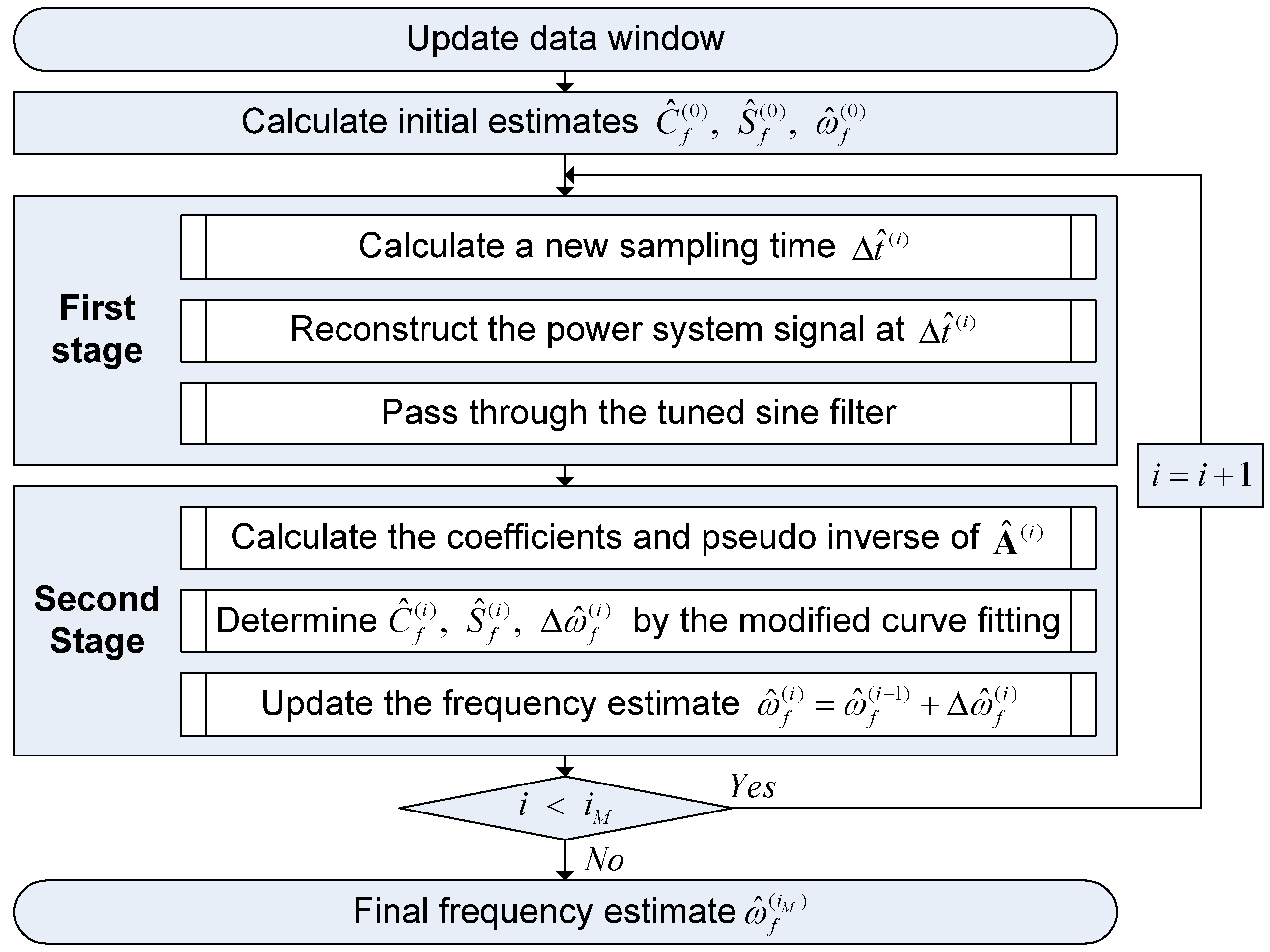
2. Two-Stage Algorithm for Estimating a Fundamental Frequency
2.1. Tuned Sine Filtering Followed by Time-Domain Interpolation
2.2. Modified Curve Fitting with an Unknown Frequency
2.3. Frequency Estimation Procedure

3. Performance Evaluation
3.1. Computer Simulations
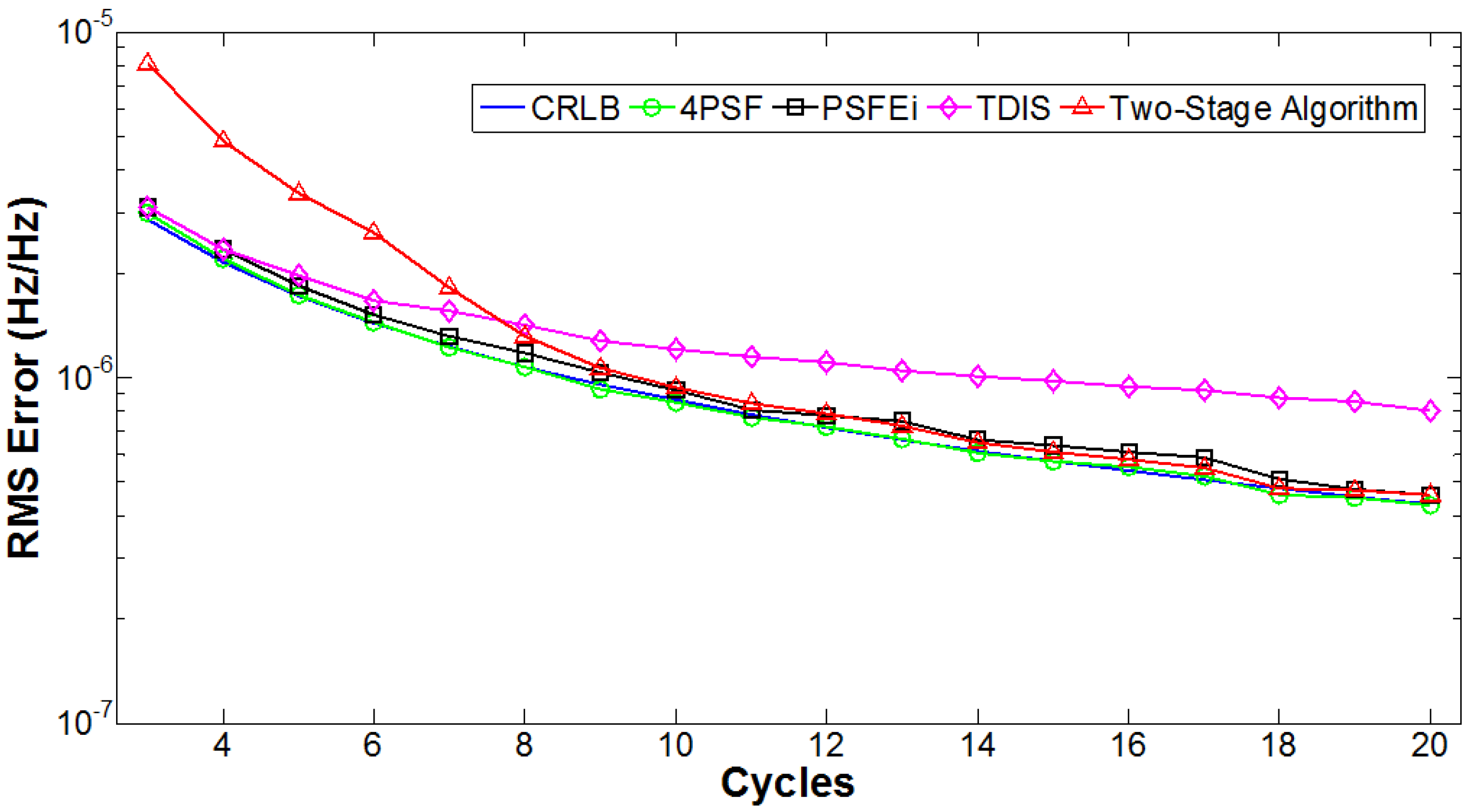
3.1.1. Number of Cycles in the Data Window

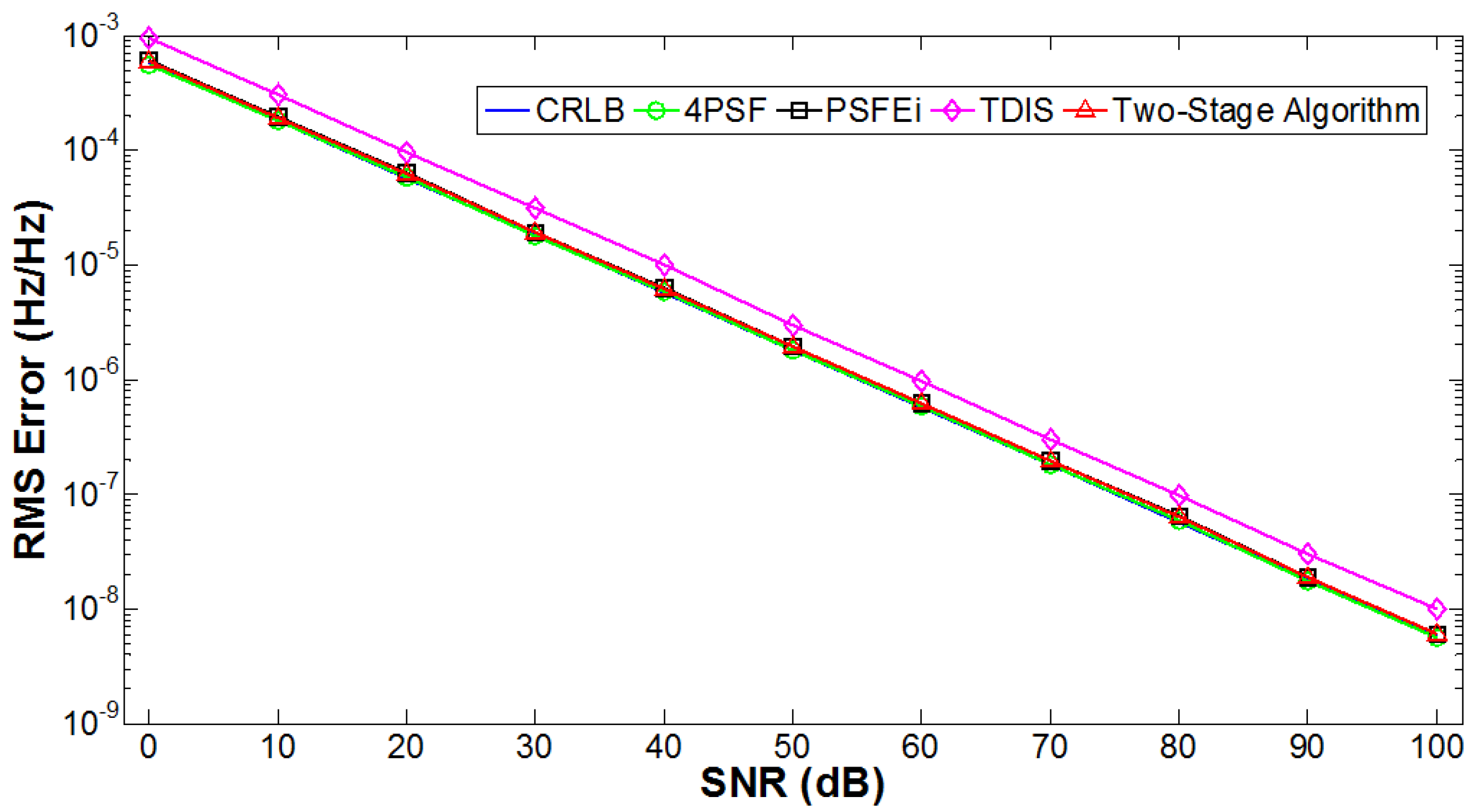
3.1.2. Noise Level

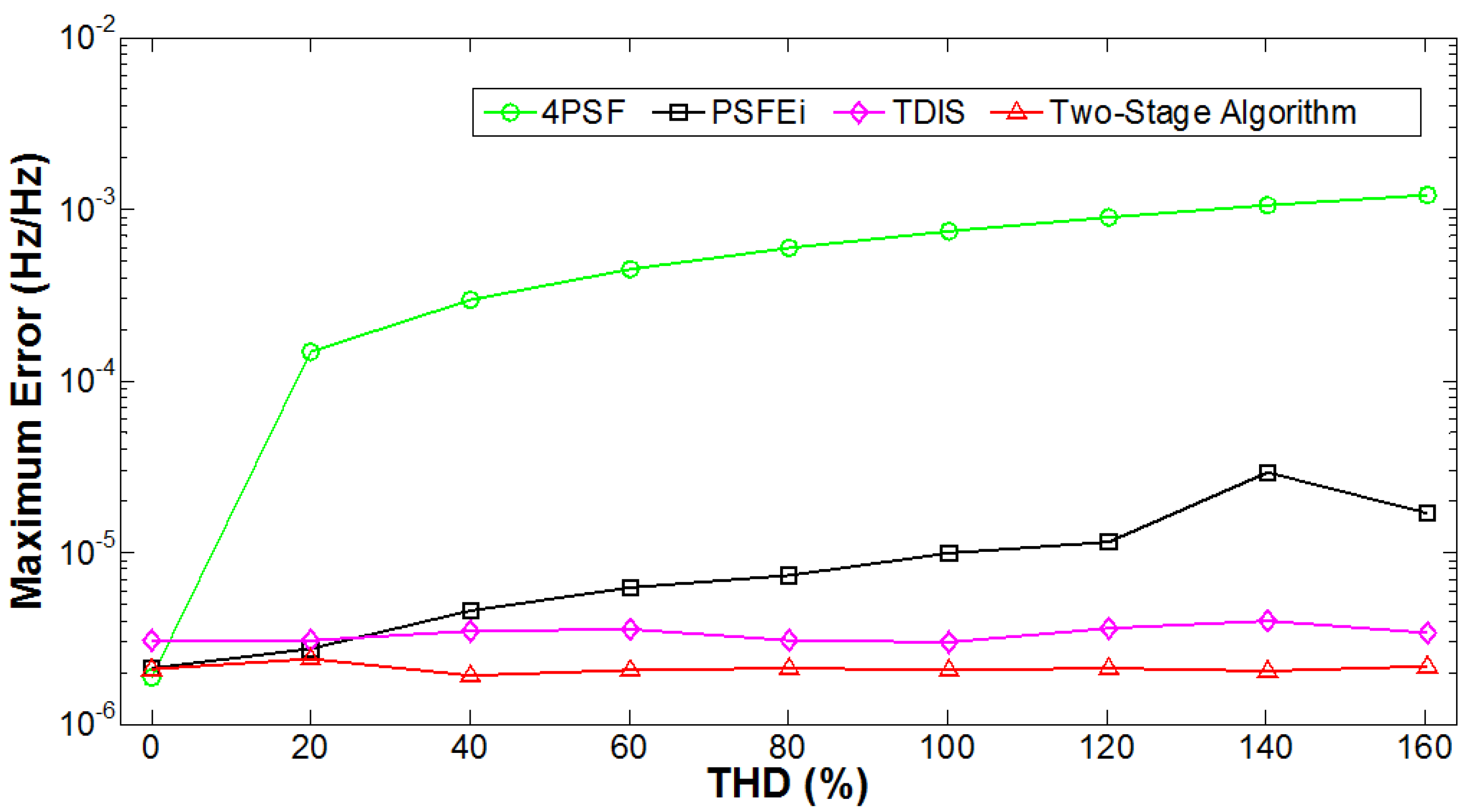
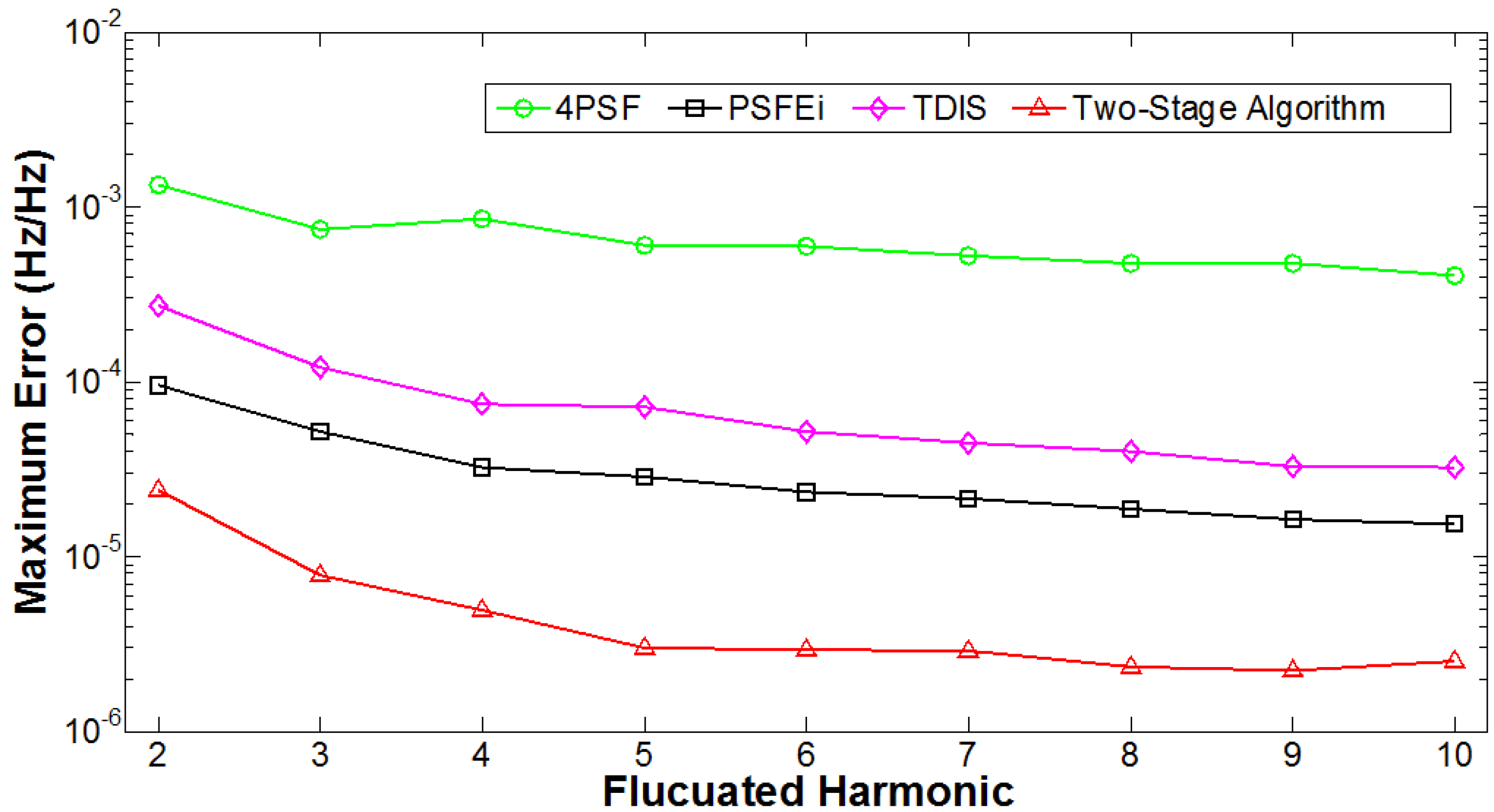
3.1.3. Harmonics

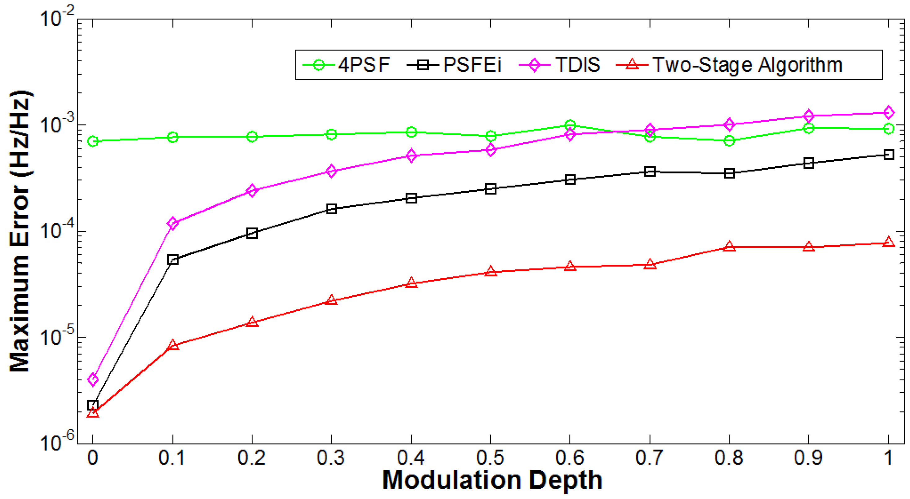
3.1.4. Fluctuating Harmonic Component


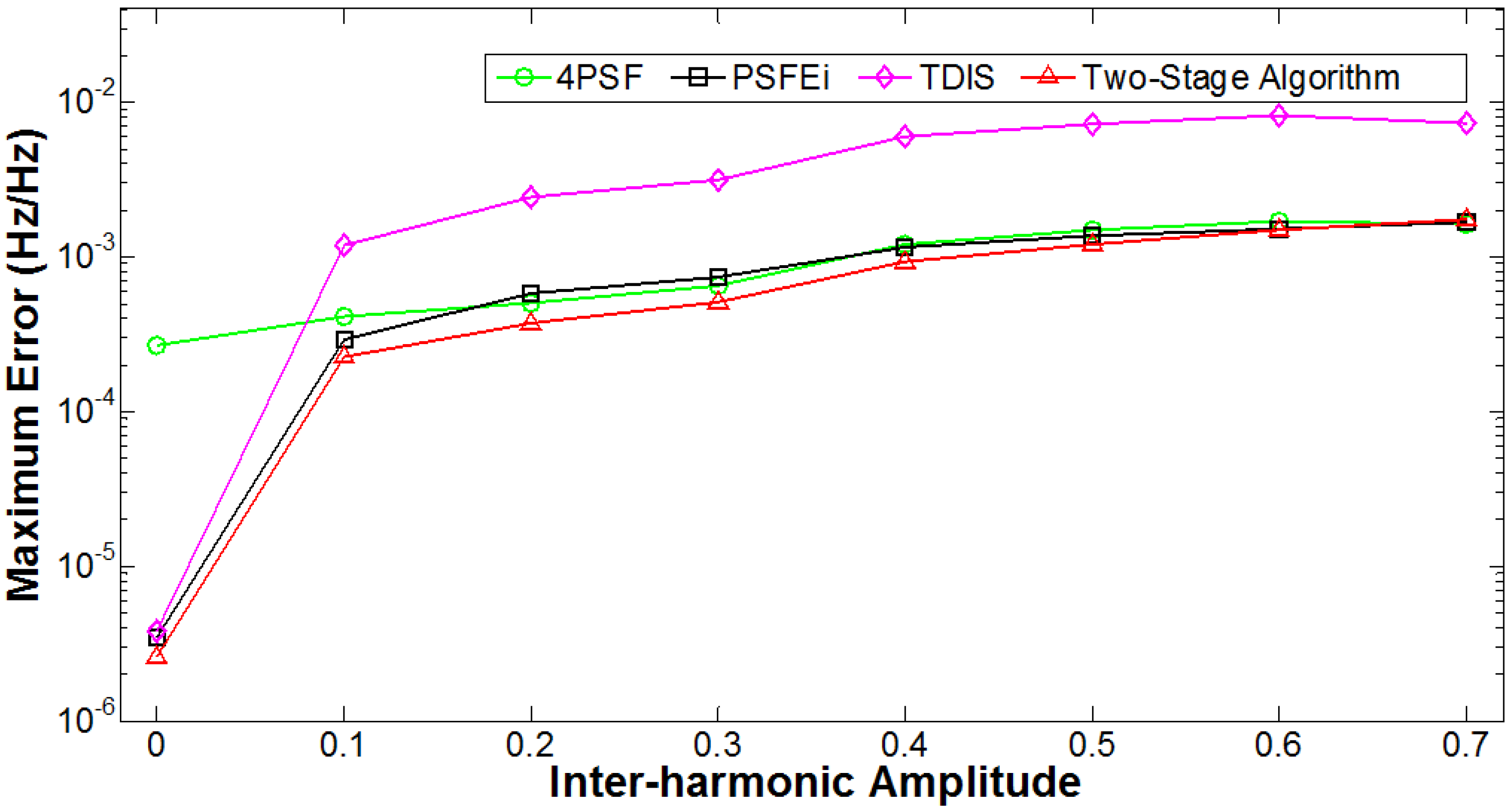
3.1.5. Fluctuating Inter-Harmonic Component

3.1.6. Computational Burden

| Algorithm | Figure number | ||||||
|---|---|---|---|---|---|---|---|
| 2 | 3 | 4 | 5 | 6 | 7 | ||
| 4PSF | 8.3337 | 8.2824 | 8.1042 | 8.3044 | 8.2134 | 8.5206 | |
| PSFEi | 12.388 | 11.279 | 10.444 | 11.102 | 10.710 | 11.762 | |
| TDIS | 463.98 | 465.78 | 459.23 | 466.76 | 462.63 | 481.13 | |
| Two-stage | 254.12 | 348.07 | 331.07 | 341.41 | 339.56 | 355.14 | |
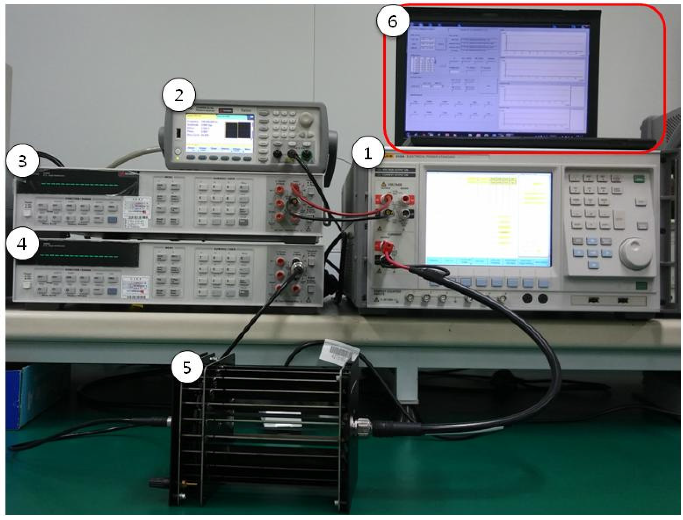
3.2. Hardware Implementation

| No. | Device Name |
|---|---|
| 1 | Electrical power quality calibrator (Fluke 6105A) |
| 2 | Waveform generator (Agilent 33500B) |
| 3,4 | Digitizing multi-meter (Agilent 3458A) |
| 5 | Current shunt (Fluke A40B) |
| 6 | Host computer |
| Voltage | H1 = 110 V, θ1 = 0 | H1 = 220V, θ1 = 0 | |||||||
|---|---|---|---|---|---|---|---|---|---|
| Harmonic | H3 = 10% | H3 = 10% | H49 = 10% | H49 = 10% | H3 = 10% | H3 = 10% | H49 = 10% | H49 = 10% | |
| θ3 = 0 | θ3 = π | θ49 = 0 | θ49 = π | θ3 = 0 | θ3 = π | θ49 = 0 | θ49 = π | ||
| 4PSF | 6.6318 | 12.492 | 9.9227 | 9.6065 | 8.7664 | 11.733 | 9.5059 | 9.7659 | |
| PSFEi | 9.4811 | 9.9378 | 9.9649 | 9.6864 | 9.6831 | 9.4355 | 9.8214 | 9.9948 | |
| TDIS | 11.623 | 8.4567 | 9.3250 | 9.1283 | 10.472 | 9.7417 | 9.0150 | 9.0917 | |
| Two-stage | 9.5266 | 9.8951 | 9.9366 | 9.6903 | 9.5992 | 9.5416 | 9.7377 | 9.9564 | |
4. Conclusions
Acknowledgments
Author Contributions
Conflicts of Interest
References
- Grandke, T. Interpolation algorithms for discrete Fourier transforms of weighted signals. IEEE Trans. Instrum. Meas. 1983, 32, 350–355. [Google Scholar] [CrossRef]
- Andria, G.; Savino, M.; Trotta, A. Windows and interpolation algorithms to improve electrical measurement accuracy. IEEE Trans. Instrum. Meas. 1989, 38, 856–863. [Google Scholar] [CrossRef]
- Xi, J.; Chicharo, J.F. A new algorithm for improving the accuracy of periodic signal analysis. IEEE Trans. Instrum. Meas. 1996, 45, 827–831. [Google Scholar]
- Zhang, F.; Geng, Z.; Yuan, W. The algorithm of interpolating windowed FFT for harmonic analysis of electric power system. IEEE Trans. Power Del. 2001, 16, 160–164. [Google Scholar] [CrossRef]
- Radil, T.; Ramos, P.M.; Serra, A.C. New spectrum leakage correction algorithm for frequency estimation of power system signals. IEEE Trans. Instrum. Meas. 2009, 58, 1670–1679. [Google Scholar] [CrossRef]
- Begovic, M.M.; Djuric, P.M.; Dunlap, S.; Phadke, A.G. Frequency tracking in power network in the presence of harmonics. IEEE Trans. Power Del. 1993, 8, 480–486. [Google Scholar] [CrossRef]
- Moore, P.J.; Carranza, R.D.; Johns, A.T. A new numeric technique for high-speed evaluation of power system frequency. IEE Proc. Gen. Transm. Distrib. 1994, 141, 529–536. [Google Scholar] [CrossRef]
- Akke, M. Frequency estimation by demodulation of two complex signals. IEEE Trans. Power Del. 1997, 12, 157–163. [Google Scholar] [CrossRef]
- Sidhu, T.S. Accurate measurement of power system frequency using a digital signal processing technique. IEEE Trans. Instrum. Meas. 1999, 48, 75–81. [Google Scholar] [CrossRef]
- Yang, J.Z.; Liu, C.W. A precise calculation of power system frequency. IEEE Trans. Power Del. 2001, 16, 361–366. [Google Scholar] [CrossRef]
- Nam, S.R.; Lee, D.G.; Kang, S.H.; Ahn, S.J.; Choi, J.H. Power system frequency Estimation in Power Systems Using Complex Prony Analysis. Int. J. Electr. Eng. Tech. 2011, 6, 154–160. [Google Scholar] [CrossRef]
- Ren, J.; Kezunovic, M. A Hybrid method for power system frequency estimation. IEEE Trans. Power Del. 2012, 27, 1252–1259. [Google Scholar] [CrossRef]
- Yamada, T. High-accuracy estimations of frequency, amplitude, and phase with a modified DFT for asynchronous sampling. IEEE Trans. Instrum. Meas. 2013, 48, 1428–1435. [Google Scholar] [CrossRef]
- Nam, S.R.; Kang, S.H.; Kang, S.H. Real-time estimation of power system frequency using a three-level discrete fourier transform method. Energies 2015, 8, 79–93. [Google Scholar] [CrossRef]
- Pintelon, R.; Schoukens, J. An improved sine-wave fitting procedure for characterizing data acquisition channels. IEEE Trans. Instrum. Meas. 1996, 45, 588–593. [Google Scholar] [CrossRef]
- Handel, P. Properties of the IEEE-STD-1057 Four-Parameter Sine Wave Fit Algorithm. IEEE Trans. Instrum. Meas. 2000, 49, 1189–1193. [Google Scholar] [CrossRef]
- Ramos, P.M.; da Silva, M.F.; Martins, R.C.; Cruz Serra, A.M. Simulation and experimental results of multi-harmonic least squares fitting algorithms applied to periodic signals. IEEE Trans. Instrum. Meas. 2006, 55, 646–651. [Google Scholar] [CrossRef]
- Ramos, P.M.; Cruz Serra, A.M. Least squares multi-harmonic fitting: Convergence improvements. IEEE Trans. Instrum. Meas. 2007, 56, 1412–1418. [Google Scholar] [CrossRef]
- Giarnetti, S.; Leccese, F.; Caciotta, M. Non recursive multi-harmonic least squares fitting for grid frequency estimation. Measurement 2015, 66, 229–237. [Google Scholar] [CrossRef]
- Zhu, L.M.; Ding, H.; Zhu, X.Y. Extraction of periodic signal without external reference by time-domain average scanning. IEEE Trans. Ind. Electron. 2008, 55, 918–927. [Google Scholar] [CrossRef]
- Clarkson, P.; Wright, P. Evaluation of an asynchronous sampling correction technique suitable for power quality measurements. In Proceedings of the IMEKO World Congress Fundamental and Applied Metrology, Lisbon, Portugal, 6–11 September 2009; pp. 907–912.
- Zhou, F.; Huang, Z.; Zhao, C.; Wei, X.; Chen, D. Time-domain quasi-synchronous sampling algorithm for harmonic analysis based on Newton’s interpolation. IEEE Trans. Instrum. Meas. 2011, 60, 2804–2812. [Google Scholar] [CrossRef]
- Wang, K.; Teng, Z.; Wen, H.; Tang, Q. Fast Measurement of Dielectric Loss Angle with Time-Domain Quasi-Synchronous Algorithm. IEEE Trans. Instrum. Meas. 2015, 64, 935–942. [Google Scholar] [CrossRef]
- Lapuh, R.; Clarkson, P.; Pogliano, U.; Hallstrom, J.K.; Wright, P.S. Comparison of asynchronous sampling correction algorithms for frequency estimation of signals of poor power quality. IEEE Trans. Instrum. Meas. 2011, 60, 2235–2241. [Google Scholar] [CrossRef]
- Ristic, B.; Boashash, B. Comments on “The Cramer-Rao lower bounds for signals with constant amplitude and polynomial phase”. IEEE Trans. Signal. Process. 1998, 46, 1708–1709. [Google Scholar] [CrossRef]
- Lapuh, R. Phase Estimation of Asynchronously Sampled Signal Using Interpolated Three-Parameter Sinewave Fit Technique. In Proceedings of the Instrumentation and Measurement Technology Conference, Austin, TX, USA, 3–6 May 2010; pp. 82–86.
- Lapuh, R. Phase Sensitive Frequency Estimation Algorithm for Asynchronously Sampled Harmonically Distorted Signals. In Proceedings of the Instrumentation and Measurement Technology Conference, Binjiang, China, 10–12 May 2011; pp. 1–4.
- Negusse, S.; Handel, P.; Zetterberg, P. IEEE-STD-1057 Three Parameter Sine Wave Fit for SNR Estimation: Performance Analysis and Alternative Estimators. IEEE Trans. Instrum. Meas. 2014, 63, 1514–1523. [Google Scholar] [CrossRef]
- Press, W.H.; Teukolsky, S.A.; Vetterling, W.T.; Flannery, B.P. Numerical Recipes in C: The Art of Scientific Computing; Cambridge University Press: Cambridge, UK, 1992. [Google Scholar]
- Souders, M.; Blair, J.; Boyer, W. IEEE Std. 1057-2007. In IEEE Standard for Digitizing Waveform Recorders; Institute of Electrical and Electronics Engineers (IEEE): New York, NY, USA, 2008. [Google Scholar]
- Agrez, D. Dynamics of Frequency Estimation in the Frequency Domain. IEEE Trans. Instrum. Meas. 2007, 56, 2111–2118. [Google Scholar] [CrossRef]
© 2015 by the authors; licensee MDPI, Basel, Switzerland. This article is an open access article distributed under the terms and conditions of the Creative Commons Attribution license (http://creativecommons.org/licenses/by/4.0/).
Share and Cite
Moon, J.-H.; Kang, S.-H.; Ryu, D.-H.; Chang, J.-L.; Nam, S.-R. A Two-Stage Algorithm to Estimate the Fundamental Frequency of Asynchronously Sampled Signals in Power Systems. Energies 2015, 8, 9282-9295. https://doi.org/10.3390/en8099282
Moon J-H, Kang S-H, Ryu D-H, Chang J-L, Nam S-R. A Two-Stage Algorithm to Estimate the Fundamental Frequency of Asynchronously Sampled Signals in Power Systems. Energies. 2015; 8(9):9282-9295. https://doi.org/10.3390/en8099282
Chicago/Turabian StyleMoon, Joon-Hyuck, Sang-Hee Kang, Dong-Hun Ryu, Jae-Lim Chang, and Soon-Ryul Nam. 2015. "A Two-Stage Algorithm to Estimate the Fundamental Frequency of Asynchronously Sampled Signals in Power Systems" Energies 8, no. 9: 9282-9295. https://doi.org/10.3390/en8099282