Optimal Siting and Sizing of Distributed Generators in Distribution Systems Considering Cost of Operation Risk

Abstract

With the penetration of distributed generators (DGs), operation planning studies are essential in maintaining and operating a reliable and secure power system. Appropriate siting and sizing of DGs could lead to many positive effects forthe distribution system concerned, such as the reduced total costs associated with DGs, reduced network losses, and improved voltage profiles and enhanced power-supply reliability. In this paper, expected load interruption cost is used as the assessment of operation risk in distribution systems, which is assessed by the point estimate method (PEM). In light with the costs of system operation planning, a novel mathematical model of chance constrained programming (CCP) framework for optimal siting and sizing of DGs in distribution systems is proposed considering the uncertainties of DGs. And then, a hybrid genetic algorithm (HGA), which combines the GA with traditional optimization methods, is employed to solve the proposed CCP model. Finally,the feasibility and effectiveness of the proposed CCP model are verified by the modified IEEE 30-bus system, and the test results have demonstrated that this proposed CCP model is more reasonable to determine the siting and sizing of DGs compared with traditional CCP model.

1. Introduction

With the continuous exhaustion of fossil energy, the gradual increase in the global temperature and the limitation of available transmission corridors, rapid development of distributed generators (DGs) has been vigorously developing around the world [1]. The subsequent growth of DGs has enabled distribution systems to actively respond to the dynamics of the main grid [2].

Although the use of DGs is helpful at many aspects, the extensive penetration of DGs could lead to some security and economic risks to active distribution networks. Specifically, the intermittency and variability of renewable-type DGs impose challenges when planning active distribution networks [3,4,5]. Inappropriate sitingand sizing of DGs could lead to many negative effects on the distribution systems concerned, such as the relay system configurations, voltage profiles, and network losses [6]. Therefore, it is becoming increasingly important of siting and sizing the DGs in active distribution networks planning.

There are various uncertainty handling methods developed for dealing with the uncertainties caused by the randomness of DGs’output [7]. These methods can be categorized into three main categories [8]: information gap decision theory (IGDT), robust restoration method and fuzzy modeling. However, the mathematical models that are obtained are mixed-integer nonlinear programming ones with multiple included variables and constraints. Chance constrained programming in [9] is powerful and robust in cases of severe uncertainty.

Many research papers on the subject of the optimal siting and sizing of DGs have become available in the past decade [10,11,12,13,14,15,16,17,18,19,20]. However, most of them are based on how to establish the objective function to obtain the maximum economic benefits. For example, in [10], an optimal distributed generation allocation on an existing MV distribution network based on genetic algorithm considering the uncertainties of DGs’ numbers, locations and capacities was proposed; in [11,12], locations and discrete capacities of DGs are determined in the view of minimizing the distribution network losses; References [13,14] determined the locations and capacities of DGs in case of minimum network losses based on an improved Hereford ranch algorithm and a combination of genetic algorithm and simulated annealing respectively. These papers only considered the network losses with the penetration of DGs, which is not adequate in determining the locations and capacities of DGs. In [15], an optimal investment planning for distributed generation in a competitive electricity market was proposed. In [16,17], a multi-objective evolutionary algorithm for the sizing and siting of distributed generation was proposed. In these papers, many costs including investment cost and network loss cost are considered but chance constraints of the established system operation planning are not considered. Also, in these papersthe only DGs considered arediesel generators and micro-turbines.

In recent years, [18] presented an chance constrained programming (CCP) framework of optimal siting and sizing of DGs with the minimization of the DGs’ investment cost, operating cost, maintenance cost, network loss cost, as well as the capacity adequacy cost. The authors of [19,20] determined the optimal location for placing the distributed generators based on loss sensitivity factor and also proposed a successive sizing based algorithm for determining their optimal sizes. In these papers, chance constraints are considered, but none of the papers mentioned above considered the costs of operation risk caused by DGs.

Many other research papers have showed that the presentation of DGs could increase the operation risk in distribution systems such as load curtailment. In [21], a hierarchical method was presented to evaluate the risk of active distribution networks considering the influence of different kinds of DGs. In [22], a novel operation risk assessment method based on credibility theory was used to assess the power system operations. Reference [23] presented a risk assessment approach to analyze power system security for operation planning under high penetration of wind power generation. These papers aimed at calculating the risk assessment of active distribution networks, which can be evaluated by expected energy not supplied (EENS) [24,25,26]. In [27,28], the unit interruption cost (UIC) is estimated, which can be used to assess the operation risk cost of distribution systems when combined with EENS.

In this paper, expected load interruption cost (ELIC) is used as the assessment of operation risk in distribution systems, which is assessed by point estimate method (PEM). In light of the costs of system operation planning, a novel chance constrained programming (CCP) framework mathematical model for optimal siting and sizing of DGs in distribution systems is proposed considering the uncertainties of DGs. Then, a hybrid genetic algorithm (HGA), which combines the genetic algorithm (GA) with traditional optimization methods, is employed to solve the proposed CCP model. This HGA overcome the drawbacks of both GA and traditional optimization methods.

Finally, the feasibility and effectiveness of the proposed CCP model are verified by the modified IEEE 30-bus system, and the test results have demonstrated that this proposed CCP model is more reasonable to determine the siting and sizing of DGs compared with traditional CCP model. Simulation results also demonstrate that the appropriate siting and sizing of DGs could lead to many positive effects on the distribution system concerned, such as the reduced total costs associated with DGs, reduced network losses, and improved voltage profiles and enhanced power-supply reliability.

2. Output Power of Distributed Generators

The dynamic output power of DGs is intricate with great volatilities and randomness, which mainly depends on the local weather condition. In distribution system, whether the load can be supplied is much related with the output power of DGs when malfunction appears, so the output power of DGs should be calculated for distributed system assessment. In this paper, wind generating units and photovoltaic generation units are considered as DGs, but it should be mentioned that the proposed optimization method in this paper could accommodate other DGs as well.

2.1. Output-Power of Wind Generating Units

The output-power of wind generating units is mainly related with the stochastic wind speed of the surroundings where wind generating units locate. In the past decades, large amounts of researches have demonstrated that the stochastic wind speed in most regions approximately follows the Weibull distribution [18,29,30], and this conclusion is employed in this paper. In general, probability density function of the stochastic wind speed can be depictedin Equation (1):

$$f_v(v)=\frac{k}{c}(\frac{v}{c})\text{exp}[-{(\frac{v}{c})}^k]$$

(1)

where k and c are, respectively, the shape index and the scale index of the Weibull distribution, which can be calculated by Maximum Likelihood Estimate and the historical data of wind speed.

In light with the known probability distribution function of the wind speed, the output power of wind generating units can be fitted as follows [31]:

$$P_{\omega }=\{\begin{array}{c}0,\\ P_N(a_1{v}^3+a_2{v}^2+a_{3}v+a_4),\\ P_N,\\ 0,\end{array}\begin{array}{c}v<v_{in}\\ v_{in}\le v<v_N\\ v_N\le v<v_{out}\\ v\ge v_{out}\end{array}$$

(2)

where, a₁, a₂, a₃ and a₄ are the fitting coefficients. P_ω and P_N are the active output power and the rated outputpower of wind generating units respectively, and v, v_N, v_in and v_out are the wind speed at the hub height of the wind unit, the rated wind speed, the cut-in wind speed, and the cut-out wind speed respectively.

2.2. Output-Power of Photovoltaic Generating Units

Many factors, such as illumination intensity I_PV, array area of photovoltaic cell A, and photoelectric conversion efficiency η, can affect the output-power of photovoltaic generating units P_PV. But, the illumination intensity is usually considered the dominant factor of affecting the output power of a solar generating source. In a certain period of time, one hour or several hours, the illumination intensity I_PV follows the Beta distribution, and its probability density function can be expressed as follows:

$$f(I)=\frac{\Gamma (\mathsf{\alpha }+\mathsf{\beta })}{\Gamma (\mathsf{\alpha })\Gamma (\mathsf{\beta })}\cdot {\left(\frac{I_{PV}}{I_{PV}^{\max }}\right)}^{\mathsf{\alpha }-1}\cdot {\left(1-\frac{I_{PV}}{I_{PV}^{\max }}\right)}^{\mathsf{\beta }-1}$$

(3)

Where α and β are the shape indexes of the Betadistribution. $I_{PV}^{\max }$ is the maximum value of I_PV, Γ is the gamma function.

Based on the known probability distribution function of the illumination intensity, the probability density function of the output-power of photovoltaic generating units can be calculated as follows [32]:

$$f(P_{PV})=\frac{\Gamma (\mathsf{\alpha }+\mathsf{\beta })}{A\cdot \mathsf{\eta }\cdot \Gamma (\mathsf{\alpha })\Gamma (\mathsf{\beta })}\cdot {\left(\frac{P_{PV}}{P_{PV}^{\max }}\right)}^{\mathsf{\alpha }-1}\cdot {\left(1-\frac{P_{PV}}{P_{PV}^{\max }}\right)}^{\mathsf{\beta }-1}$$

(4)

where, $P_{PV}^{\max }$ is the maximum value of P_PV. P_PV is the output of photovoltaic generating units, which can bedescribed as P_PV = A·η·I_PV. As can be shown in Equation (4), the output-power of photovoltaic generating units P_PV follows the beta distribution B(α, β).

3. Cost of Risk Assessment

3.1. Cost of System Operation Risk Level

The classic definition of power system reliability is related to the existence of sufficient facilities within the system so that it is capable of supplying electric power to its customers with an acceptable assurance of continuity and quality. The reliability performance of a distribution system can be measured at each customer connection point and for the whole system or any group of customers. In [26], SAIFI (system average interruption frequency index), SAIDI (system average interruption duration index) and EENS are used as reliability assessment indexes in active distribution network. In [21], four risk indices, including EENS, PLC (probability of load curtailment), EFLC (expected frequency of load curtailment) and SI (severity index), are adopted to evaluate the system operation risk level. It should be noted that EENS (expected energy not supplied, MWh/year) is one of the most important parameters to reflect the risk level of transmission system. In this paper, the assessment of system operation risk level is measured by the amount of expected load interruption cost (ELIC), which is the product of the unit interruption cost (UIC) in $/kWh and the expected energy not supplied (EENS).

$$\text{ELIC}=\text{UIC}\times \text{EENS}$$

(5)

The UIC can be estimated by a method based on the revenue lost to a utility due to power outages [27]. The index of EENS (expected energy not supplied, MWh/year) is calculated by Equation (6):

$$\text{EENS}={\displaystyle \sum _{i=1}^{N_L}({\displaystyle \sum _{s\in Q_i}{p}_T(s)}\cdot C_0(s))}\cdot T_i$$

(6)

where, N_L is total number of load levels; T_i is the durationof load level i; Q_i is system state set for load leveli; p_T(s) is occurrence probability of system state s; C₀(s) is total load curtailment in system state s.

3.2. Costs of System OperationPlanning

The costs of system operation planning can consists of many aspects, such as the investment cost, operating cost, maintenance cost, network loss cost, and capacity adequacy cost. Capacity adequacy cost can be reflected by ELIC to some degree, and operating cost for a renewable DG is zero. Furthermore, the installed DGs in a distribution systems will bring a benefit to distribution systems, which is to generate electricity replacing conventional fossil energy. As a result, the generation cost replaced by DGs should be considered in the costs of system operation planning.

Therefore, investment cost C^I, maintenance cost C^M, network loss cost C^L, and the generation cost C^DG replaced by DGs are used for the costs of system operation planning, which can be depicted as Equation (7):

$$C_{DG}=C^I+C^M+C^L-C^{DG}$$

(7)

In [33,34,35], many methods have been used to calculate the indexes of investment cost, maintenance cost, and network loss cost. In this paper, network loss cost C^L can be depicted as Equation (8), the investment cost C^I can be depicted as Equation (9), the maintenance cost C^M can be depicted as Equation (10), the generation cost C^DG replaced by DGs can be depicted as Equation (11):

$$C^L={\displaystyle \sum _{j=1}^L{C}_e{\mathsf{\tau }}_{j\max }{R}_j\frac{P_j}{{(U_N{\mathsf{\lambda }}_j)}^2}}$$

(8)

In Equation (8), C_e is the unit electricity saleprice ($·kW⁻¹), τ_jmax is the maximum hours of load loss in branch j, and R_j is the resistance of branch j. P_j is the active power that flows through branch j, U_N is the rated voltage of line j, and λ_j is the load power factor of branch j:

$$C^I={\displaystyle \sum _{i=1}^N{\displaystyle \sum _{m=1}^2{a}_{i}E\cdot P_{i-\max }\cdot C_{OMi}^m\cdot \frac{r{(1+r)}^{n_{DG}}}{{(1+r)}^{n_{DG}}-1}}}$$

(9)

In Equation (9), $C_{OMi}^m$ represents the per-unit capacity investment cost of the DG m at node i, and N is the number of candidate node. a_i = f(x₁, x₂, x₃) is the weighting coefficients of investment cost, which relates to environmental factor x₁, displacement factor x₂, transportation and labor cost factor x₃. r is the discount rate, and n_DG is the lifetime of DGs. P_i-max is the upper limits of DGs capacities in candidate node i, and E is candidate DG capacity in candidate node i, which will be introduced in Section 4.2:

$$C^M={\displaystyle \sum _{i=1}^N{\displaystyle \sum _{m=1}^2{T}_{\max }\cdot C_{OPi}^m\cdot E\cdot P_{i-\max }}}$$

(10)

In Equation (10), T_max is the maximum hours of DGs generation, N is the number of DGs, and $C_{OPi}^m$ represents the per-unit capacity maintenance cost of the DG m at node i:

$$C^{DG}={\displaystyle \sum _{i=1}^N{\displaystyle \sum _{m=1}^{2}E\cdot P_{i-\max }\cdot {\mathsf{\eta }}_i\cdot T_{eq}\cdot C_{en}^m}}$$

(11)

In Equation (11), T_eq is the equivalent generation hours of DGs generation, and $C_{en}^m$ is the unit on-grid electricity price of DG m. η_i is the efficiency of DG m in node i.

4. Mathematical Model

4.1. Methodological Framework

The developed mathematical model of the CCP-based optimal siting and sizing of DGs in this paper can be formulated as:

$$\begin{array}{ll}\min & f(E,X)\\ s.t.& P_r\left\{g_j(E,X)\le 0\right\}\ge \mathsf{\lambda }(j=1,2,\cdots ,N_L)\\ & \begin{array}{c}G=0\end{array}\\ & H_{\min }\le H\le H_{\max }\end{array}$$

(12)

where, f(E, X) is the objective function, g_i(E, X) are chance constraints, G = 0 represents the equality constraints, and H_min ≤ H ≤ H_max is the inequality constraints. E is the decision-making vector; X is a set of stochastic variables with known probability. λ is the given confidence levels; N_L is the number of feeders in the distribution system; H_min/H_max is the set of the minimal/maximal limits of inequality constraints.

4.2. Objective Function

In order to obtain the optimal locations and capacities of DGs, the optimization variable included in the planning scheme should be constructed.

Suppose that m represents the species of DGs in the distribution system. m = 1/2 represent wind generating units and photovoltaic generating units, respectively. If y represents the installed capacities of DGs in the distribution system, then y_m1, y_m2, …, y_mn can represent the candidate locations and installed capacities for DGs in the distribution system. y_mi (i = 1,2, …, N) = 0 denotes that there will not be a DG m built at candidate nodes i (i = 1, 2, …, N). y_mi (i = 1, 2, …, n) > 0 denotes that there will be a DG m built at candidate nodes i (i = 1, 2, …, n), and the installed capacity is y_mi.

Furthermore, the installed capacities of DGs could be normalized, namely y_mi = y_mi/P_i-max. Thence, the stochastic variables E in Equation (10) can be depicted as:

$$E=\left\{y_{mi}|i=1,2,\cdots ,N;m=1,2\right\}$$

(13)

In this paper, the objective function is described as:

$$\min \begin{array}{c}f\end{array}={\mathsf{\alpha }}_1{C}_{DG}+{\mathsf{\alpha }}_2\cdot \text{ELIC}$$

(14)

where, α₁, α₂ are the weighting coefficients. C_DG is the costs of system operation planning associated with the DGs, which can be calculated by Equation (7). ELIC is the costs caused by EENS, which can be calculated by Equation (5).

4.3. Network Constraints

As shown in Equation (12), there are three kinds of network constraints, including equality constraints, inequality constraints, and chance constraints.

(1) The equality constraints include the well-known load-flow equations, which can be depicted in Equation (15):

$$\{\begin{array}{c}{P}_{is}=U_i{\displaystyle \sum _{j\in i}{U}_j(G_{ij}\cos {\mathsf{\theta }}_{ij}+B_{ij}\cos {\mathsf{\theta }}_{ij})}\\ Q_{is}=U_i{\displaystyle \sum _{j\in i}{U}_j(G_{ij}\cos {\mathsf{\theta }}_{ij}-B_{ij}\cos {\mathsf{\theta }}_{ij})}\end{array}$$

(15)

where, P_is and Q_is are the total active, reactive output power of the generators at node i, U_i and U_j are the voltage amplitude at node i and j respectively. G_ij and B_ij are the conductance and susceptance between node i and j respectively. θ_ij is the voltage angle between node i and j.

For E, if y_1i > 0, y_2i = 0; if y_2i > 0, y_1i = 0. Namely, wind generating units and photovoltaic generating units cannot be installed in node i simultaneously. Therefore, an additional equality constraint is included in the equality constraints in this paper, which is shown in Equation (16):

$$y_{1i}\cdot y_{2i}=0(i=1,2,\cdots ,N)$$

(16)

(2) The inequality constraints include the given permitted penetration capacity of DGs in the distribution system and the upper limits of DGs capacities in candidate node i, which are shown in Equations (17) and (18) respectively:

$${\displaystyle \sum _{i=1}^N{\displaystyle \sum _{m=1}^2{y}_{mi}\cdot P_{i-\max }}}\le P_{D{G}_{\max }}$$

(17)

$$0\le y_{mi}\le 1\begin{array}{cc},& \forall i\in N\end{array};m=1,2$$

(18)

where, P_DGmax is given permitted penetration capacity of DGs in the distribution system.

(3) The chance constraints in this paper mainly include node voltage constraints and branch transmission power constraints, which are shown in Equations (19) and (20) respectively:

$$P_r\left\{U_i^{\min }\le U_i\le U_i^{\max }\right\}\ge {\mathsf{\beta }}_u\begin{array}{cc},& i=1,2,\cdots ,N_b\end{array}$$

(19)

$$P_r\left\{\left|P_i\right|\le P_i^{\max }\right\}\ge {\mathsf{\beta }}_p\begin{array}{cc},& i=1,2,\cdots ,N_a\end{array}$$

(20)

where,{·} represents the probability of a certain event occurs. N_b is the total number of nodes in the distribution system, and N_a is the total number of branches in the distribution system. $U_i^{\min }$ and $U_i^{\max }$ are the upper and lower limits of the voltage U_i in node i respectively. β_u is the given confidence level of node voltage constraints, and β_p is the given confidence level of branch transmission power constraints. P_i is the transmission power in branch i, and $P_i^{\max }$ is upper limits of transmission power in branch i.

5. Solving Strategies

To solve the developed mathematical model of the CCP-based optimal siting and sizing of DGs in Equation (10), three steps are needed, as shown in Figure 1. In Step A, expected load interruption cost ELIC is calculated according to the output of wind generating units, photovoltaic generating units, and energy storage system. In Step B, total costs associated with the DGs C_DG are calculated according to the output of wind generating units, photovoltaic generating units, and energy storage system. In Step C, the objective function of optimal siting and sizing of DGs is firstly set up based on ELIC and C_DG.Then, with the network constraints, the developed mathematical model of the CCP-based optimal siting and sizing of DGs is solved, and the optimal solution E* is obtained.

Figure 1. Flowchart of the developed chance constrained programming (CCP)-based method for optimal siting andsizing of distributed generators(DGs) in distribution systems.

Figure 1. Flowchart of the developed chance constrained programming (CCP)-based method for optimal siting andsizing of distributed generators(DGs) in distribution systems.

5.1. Calculation of Expected Load Interruption Cost (ELIC)

In [21], a hierarchical risk assessment method based on discrete probability model of DGs, the enumeration method and Monte Carlosimulation was proposed to calculate EENS. This method is much effective, but is relatively complex. In [36], point estimate method (PEM) was used for transmission line overload risk assessment. This method is much effective, but is relatively complex. Compared with Monte Carlosimulation, PEM is slightly low in accuracy, but the computational cost of PEM is largely reduced. Therefore, point estimate method (PEM) is used to calculate the EENS parameterin this paper:

(1) The point estimate method (PEM), proposed by Hong in 1998, is used to calculate the estimation value E(Z^j) of F(X) (Z = F(X) = F(X₁, X₂, …, X_m)) when the probability distribution functions of random variables X = (X₁, X₂, …, X_m) are known [37,38]. The mathematical principle of PEM can be depictedin Equation (21):

$$E(Z^j)\approx {\displaystyle \sum _{l=1}^m{\displaystyle \sum _{k=1}^K{\mathsf{\omega }}_{l,k}{F}^j({\mathsf{\mu }}_{X1},\cdots ,x_{l,k},\cdots ,{\mathsf{\mu }}_{Xm})}}$$

(21)

where, ω_l,k is the weights of random variable X_i in x_l,k, and ${\mathsf{\mu }}_{X_i}$ is the mathematical expectation of random variable X_i. In this paper, random variable X_i is the wind speed v or illumination intensity I_PV of DG i. X_i = {X_mi|i = 1, 2, …, N; m = 1, 2}, and X_1i is the wind speed v, X_2i is illumination intensity I_PV. x_l,k can be got by Equation (22):

$$x_{i,k}={\mathsf{\mu }}_{X_i}+{\mathsf{\xi }}_{i,k}{\mathsf{\sigma }}_{X_i},i=1,2,\dots ,m,k=1,2,\dots ,2K-1$$

(22)

where, ${\mathsf{\sigma }}_{X_i}$ is the mathematical variance of random variable X_i. The values of ξ_i,k and ω_l,k can be obtained by Equation (23):

$$\{\begin{array}{c}{\displaystyle \sum _{k=1}^K{\mathsf{\omega }}_{i,k}\cdot {{\mathsf{\xi }}_{i,k}}^j}={\mathsf{\lambda }}_{i,j}\begin{array}{cc},& j=1,\cdots ,2K-1\end{array}\\ {\mathsf{\lambda }}_{i,j}=E\left[{(x_i-{\mathsf{\mu }}_{X_i})}^j\right]/{{\mathsf{\sigma }}_{X_i}}^j\end{array}$$

(23)

When K = 3, and ${\mathsf{\xi }}_{i,3}=0$ (2m + 1 PEM), Equation (23) can be solved as Equation (24):

$$\begin{array}{l}{\mathsf{\xi }}_{i,1}=\frac{{\mathsf{\lambda }}_{i,3}}{2}+\sqrt{{\mathsf{\lambda }}_{i,4}-\frac{3}{4}{{\mathsf{\lambda }}_{i,3}}^2}\\ {\mathsf{\xi }}_{i,2}=\frac{{\mathsf{\lambda }}_{i,3}}{2}-\sqrt{{\mathsf{\lambda }}_{i,4}-\frac{3}{4}{{\mathsf{\lambda }}_{i,3}}^2}\\ {\mathsf{\omega }}_{i,1}=\frac{1}{{\mathsf{\xi }}_{i,1}({\mathsf{\xi }}_{i,1}-{\mathsf{\xi }}_{i,2})},{\mathsf{\omega }}_{i,2}=-\frac{1}{{\mathsf{\xi }}_{i,2}({\mathsf{\xi }}_{i,1}-{\mathsf{\xi }}_{i,2})}\\ {\mathsf{\omega }}_{i,3}=\frac{1}{m}-\frac{1}{{\mathsf{\lambda }}_{i,4}-{{\mathsf{\lambda }}_{i,3}}^2}\end{array}$$

(24)

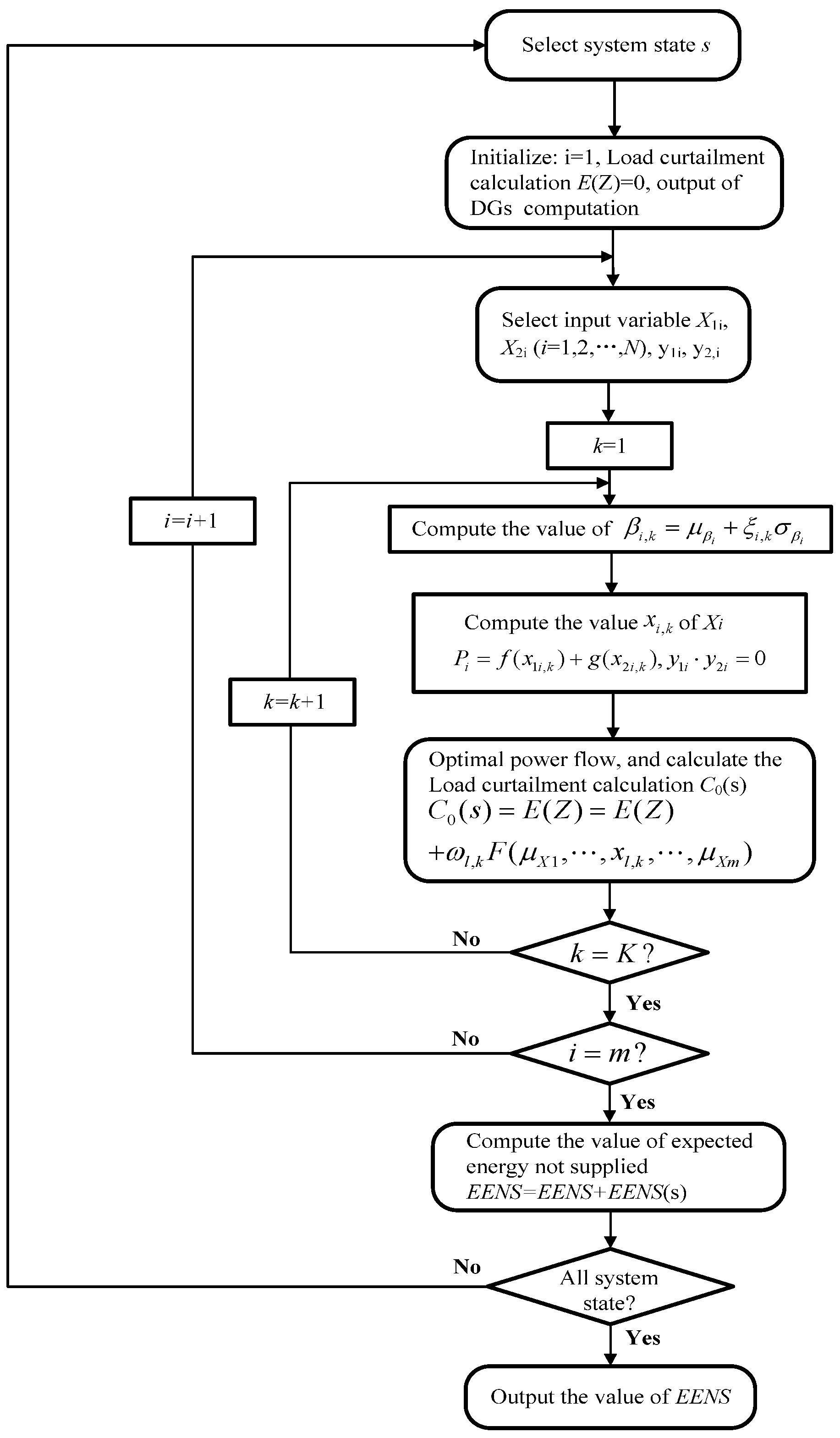
(2) The procedure for computing the index of EENS is summarized in Figure 2. In Figure 2, the 2m + 1 point estimate method (PEM) was used, namely K=3. $f(x_{1i,k})$ is calculated by Equation (2), in which P_N = y_1i·P_i-max. $g(x_{2i,k})=A\cdot \mathsf{\eta }\cdot x_{2i,k}$, and $A\cdot \mathsf{\eta }\cdot I_{PV}^{\max }=y_{2i}\cdot P_{i-\max }$. y_1i and y_2i satisfy the equality constraint Equation (16).

Figure 2. Flow chart of computing procedure for expected energy not supplied (EENS).

Figure 2. Flow chart of computing procedure for expected energy not supplied (EENS).

Also, optimal power flow was used to calculate the index of load curtailment calculation C₀(s), which was described in [39]. Due to the limited space of this paper, the detailed process of optimal power flow is not covered.

(3) The UIC can be estimated by several methods such as a method based on customer damage functions or a method based on the revenue lost to a utility due to power outages [23]. In this paper, UIC is estimated by a method based on the revenue lost to a utility due to power outages, which can be referred in [27]. In light with EENS and UIC, the value of expected load interruption cost (ELIC) can be calculated by Equation (5).

5.2. Calculation of System Operation Planning Cost

As shown as Section 3.2, network loss cost C^L, investment cost C^I, maintenance cost C^M and the generation cost C^DG replaced by DGs can be calculated by Equations (8)–(11), respectively. The system operation planning cost C_DG can be calculated by Equation (7).

It should be noted that the output power of wind generating units and photovoltaic generating units in year are generated on an hourly basis. The unit electricity sale price C_e in Equation (8) and the unit on-grid electricity price $C_{en}^m$ of DG m in Equation (11) are not constant, but can be approximately calculated by average prices of last year.

5.3. Solving Strategy of Chance Constrained Programming (CCP)-Based Optimization

In [40,41], a particle swarm optimization (PSO) algorithm is used to solve the CCP-based optimization described by Equation (12). In [18], a Monte Carlo simulation embedded genetic-algorithm approach is employed to solve the optimization problem described by Equation (12). The PSO algorithm requires a better set of initial values for the design variables and may easily fall into local optimum. GA can locate the solution in the whole domain, but it does not solve constraint problems easily, especially for exact constraints.

In order to overcome these drawbacks above, a hybrid genetic algorithm (HGA) [42], which combines the GA with traditional optimization methods, is used for solving the CCP-based optimization described by Equation (12) in this paper. In the first step of HGA, the GA is applied to provide a set of initial design variables, thereby avoiding the trial process. Thereafter, traditional algorithms are employed to determine the optimum results. The procedure for CCP-based optimization based on HGA is described as Figure 3.

Figure 3. Flow chart of hybrid genetic algorithm (HGA) for CCP-based optimization procedure.

Figure 3. Flow chart of hybrid genetic algorithm (HGA) for CCP-based optimization procedure.

In Step C of Figure 1, objective function f is firstly got by system operation planning cost C_DG and expected load interruption cost ELIC. And then, chance constraints based on Equations (16) and (17) should be checked [43]. The detailed solving steps for CCP-based optimization based on HGA are as follows:

• Specify the parameters associated with the GA, including the population size N_P, the crossover P_C, the mutation P_M and the maximum-permitted generation number N_C.
• Randomly generate N_P chromosomes.
• Update these chromosomes according to the crossover P_C and the mutation P_M.
• Check the feasibility of all chromosomes until all the chromosomes are feasible. In this procedure, all network constraints including chance constraints should be checked for the chromosomes. In this paper, check of chance constraints is based on Monte Carlo simulation procedure, which was introduced in [18] in detail.
• Repeat Steps b–e until the generation number reaches N_C.
• All the chromosomes in e are regarded as E.
• Calculate the objective function value of all chromosomes and the fitness value of each chromosome.
• Select the best chromosome found in the above solving procedure as E*.

6. Case Studies

To demonstrate the performance of the proposed model and method, it is applied to the modified IEEE 30-bus system shown in Figure 4. The parameters of wind generating units and photovoltaic generating units are given below, and other characteristic parameters are given in [44]. The base value is 100 MVA. For photovoltaic nodes, upper and lower voltage bounds are 1.1 and 0.95 p.u. and upper and lower voltage bounds are 1.06 and 0.94 p.u. for all other nodes. All case studies are carried out using MATLAB on an Advanced Micro Devices 64 Dual Core CPU 3.3 GHz PC (Lenovo, Wuhan, China).

Figure 4. DGs connected to the IEEE 30-bus system.

Figure 4. DGs connected to the IEEE 30-bus system.

The candidate notes for the species and maximum installed capacity of DGs are shown in Table 1. In Table 1, 1 and 2 represent wind generating units and photovoltaic generating units respectively. For different candidate notes, the weighting coefficients of investment cost a_i = f(x₁, x₂, x₃) is different, which is also list in Table 1. In addition, the maximum total generation capacity of DGs in the IEEE 30-bus system accounts for 30% of total load.

Table 1. Candidate notes for the species and maximum capacity of DGs.

Candidate Notes	Species m	Maximum Installed Capacity of DG m/(MW)	ai
3	1, 2	30, 20	1.01
7	1, 2	20, 20	1.03
14	1, 2	20, 20	1.05
19	2	20, 20	1.05
24	1, 2	20, 20	1.03
26	1, 2	30, 30	1.04
30	1, 2	20, 20	1.02

Table 1. Candidate notes for the species and maximum capacity of DGs.

Candidate Notes	Species m	Maximum Installed Capacity of DG m/(MW)	ai
3	1, 2	30, 20	1.01
7	1, 2	20, 20	1.03
14	1, 2	20, 20	1.05
19	2	20, 20	1.05
24	1, 2	20, 20	1.03
26	1, 2	30, 30	1.04
30	1, 2	20, 20	1.02

In all case studies, the per-unit capacity investment costs and per-unit capacity maintenance costs for wind generating units and photovoltaic generating units are shown in Table 2. To facilitate the calculation and simplify the model of Equation (12), electricity price is considered constant in one year, which can be estimated by the average value of last year. In this case, the unit electricity sale price C_e is 0.07 $/kW·h. The unit on-grid electricity prices for wind generating units and photovoltaic generating units are also list in Table 2, in which government subsidies are considered.

Table 2. The per-unit capacity Cost of DGs.

m	Investment Costs /$·kW−1	Maintenance Costs /$·(kW·h)−1	On-Gridprice /$·(kW·h)−1
1	1200	0.04	0.13
2	1400	0.03	0.15

Table 2. The per-unit capacity Cost of DGs.

m	Investment Costs /$·kW−1	Maintenance Costs /$·(kW·h)−1	On-Gridprice /$·(kW·h)−1
1	1200	0.04	0.13
2	1400	0.03	0.15

6.1. Calculation of ELIC

By the procedure for computing the index of EENS and the estimated value of UIC in Figure 2, the value of ELIC can be calculated. In this case, UIC is chosen as 0.32 $/kW·h, which is also considered constant in one year.

For the wind generation units, v_N = 15 m/s, v_in = 4 m/s, v_out = 20 m/s. The shape index k = 6.25, the scale index c = 10.45, and the fitting coefficients a₁ = 0.0014848, a₂ = −0.041545, a₃ = 0.43333 and a₄ = −1.1636. For the photovoltaic generation units, the shape indexes α = 15.34, β = 4.2, A = 2.16 m, η = 13.44%.

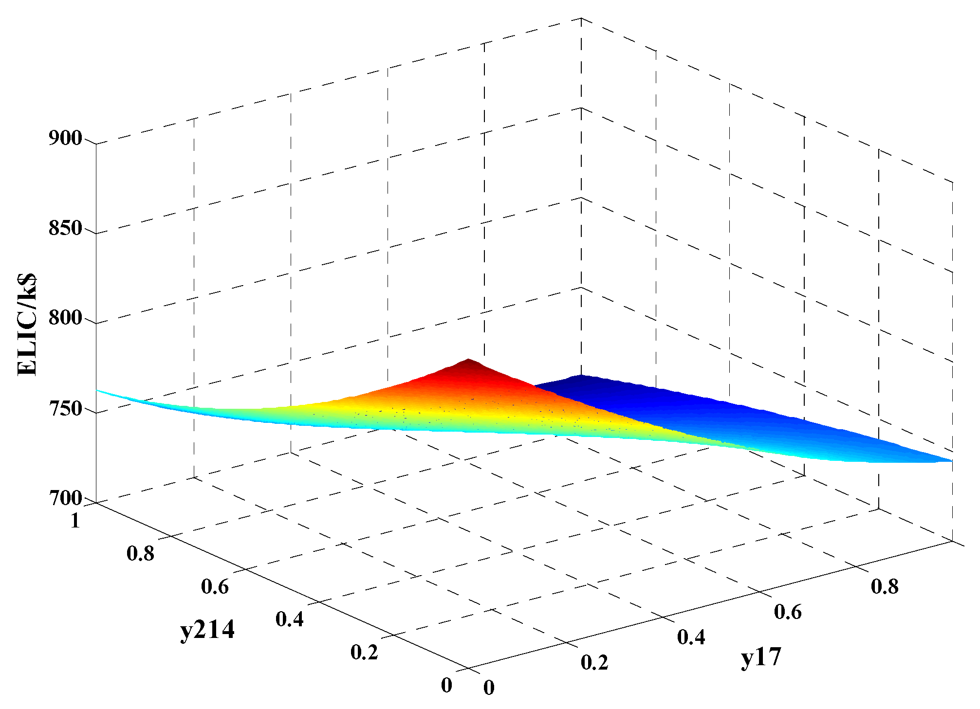
For instance, wind generating units and photovoltaic generating units are installed in note 7, 14 respectively. Then, the value of ELIC was calculated by 2m + 1 point estimate method (PEM), which is shown in Figure 5.

Figure 5. The value of ELIC impace with y₁₇ and y₂₁₄.

Figure 5. The value of ELIC impace with y₁₇ and y₂₁₄.

As can be seen from Figure 5, ELIC decreases with the increment of DGs’ capacity. When y₁₇ = 1 and y₂₁₄ = 1, the value of ELIC reach its minimum value, which is about 701.08 k$. On the other hand, the locations of DGs also affect the value of ELIC. For instance, if wind generating units and photovoltaic generating units are installed in note 19, 30 respectively, the value of ELIC is shown in Figure 6.

Figure 6. The value of ELIC impace with y₁₁₉ and y₂₃₀.

Figure 6. The value of ELIC impace with y₁₁₉ and y₂₃₀.

Compared to Figure 5, although DGs’ capacity has no changes, the value of ELIC changes when the locations of DGs change. For an example, ELIC = 701.08 k$ when y₁₇ = 1 and y₂₁₄ = 1, but ELIC = 686.55 k$ when y₁₁₉ = 1 and y₂₃₀ = 1. In addition, the distribution of DGs also affects the value of ELIC. Generally, ELIC decreases with the distribution of DGs. That is to say, the value of ELIC will be larger with more DGs connected to IEEE 30-bus system although the total capacity of DGs is constant.

In addition, it also indicates that wind generating units' power support is with better effectiveness than photovoltaic generating units, because the value of ELIC when y₁₇ = 0 and y₂₁₄ = 1 is much bigger than the value of ELIC when y₁₇ = 1 and y₂₁₄ = 0.

6.2. Calculation of System Operation Planning Cost

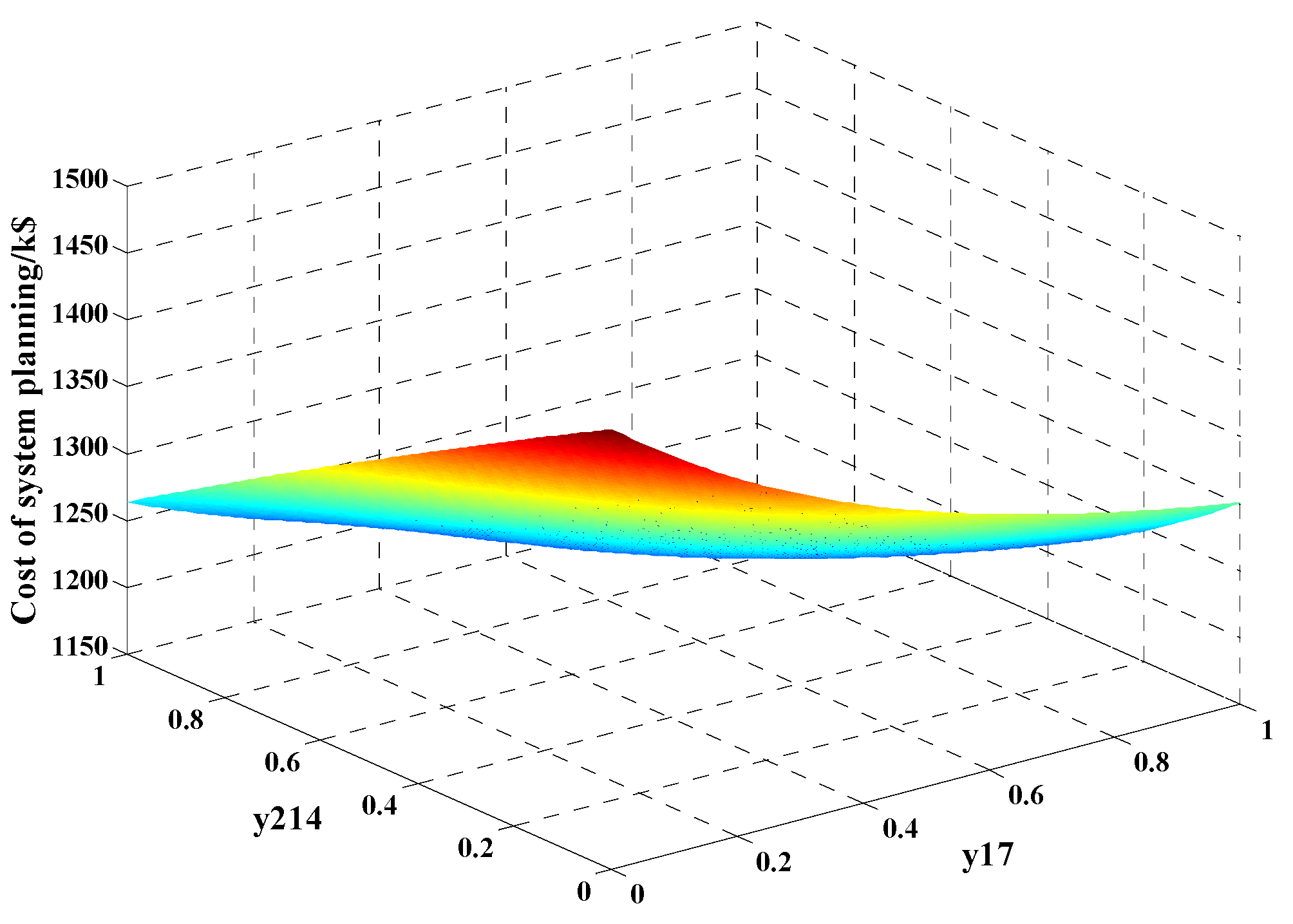
According to Section 5.2, the system operation planning cost C_DG can be calculated by Equation (7). The maximum hours of load loss in branch j τ_jmax = 3000 h, the discount rate r = 0.12, and the lifetime of DGs n_DG = 5. The equivalent generation hours of DGs generation T_eq = 3000 h. For instance, wind generating units and photovoltaic generating units are installed in note 7, 14 respectively. Then, the value of cost C_DG can be shown in Figure 7, in which all network constraints are satisfied.

Figure 7. The value of C_DG impace with y₁₇ and y₂₁₄.

Figure 7. The value of C_DG impace with y₁₇ and y₂₁₄.

As can be seen in Figure 7, the value of system operation planning cost C_DG = 1478.27 k$ when y₁₇ = 0 and y₂₁₄ = 0, in which C^L = 1478.27 k$, C^I = 0, C^M = 0, C^DG = 0. In pace with the increase of DGs’capacity y₁₇ and y₂₁₄, system operation planning cost C_DG will cut down at a certain range. When y₁₇ = 1 and y₂₁₄ = 1, cost C_DG reach its minimum value 1186.56 k$, in which C^L = 1203.63 k$, C^I = 5487.65 k$, C^M = 3741.25 k$, C^DG = 9245.97 k$.

This result shows that the installed capacities of DGs are not adequate. Namely, system operation planning cost C_DG can further cut down with the increase of DGs’capacities. In addition, it also shows that the locations of node 7 and 14 may not be the suitable locations for optimalsiting of DGs. Namely, the locations of DGs also affect the value of system operation planning cost C_DG. Anyway, the value of system operation planning cost C_DG can reach its minimum value when y_mi is at a certain fixed value for optimal sizing and siting of DGs.

6.3. Solving Strategy of CCP-Based Optimization

According to Section 5.3, an embedded genetic-algorithm approach is employed to solve the optimization problem described by Equation (12). In the objective function which is shown in Equation (14), the weighting coefficients α₁ and α₂ can greatly affect the optimization results of Equation (12). Therefore, the optimization problem described by Equation (12) is solved in four cases. In case 1, α₁ = 1 and α₂ = 0, which means that ELIC is not considered and this optimization of Equation (12) is the traditional method for optimal siting and sizing of distributed generators in distribution systems. In case 2, α₁ = 0.7 and α₂ = 0.3. In case 3, α₁ = 0.5 and α₂ = 0.5. In case 4, α₁ = 0 and α₂ = 1, which means that system operation planning cost C_DG is not considered. In all the cases, the parameters are specified as follows: N_C = 1000, N_P = 30, P_C = 0.3. Optimal sizing and siting results of DGs in cases 1–4 are shown in Table 3.

Table 3. Optimal sizing and siting of DGs in case n.

Notes	Species m of DGs	Optimal Sizing of DGs in Case n
		1	2	3	4
3	1	18.56	17.33	17.19	15.28
	2	0	0	0	0
7	1	0	0	0	7.11
	2	12.68	0	0	0
14	1	0	0	0	13.26
	2	0	0	0	0
19	1	0	0	9.07	14.52
	2	0	16.91	0	0
24	1	0	0	0	5.81
	2	0	0	0	0
26	1	0	0	0	11.77
	2	0	0	18.35	0
30	1	17.27	18.44	15.67	17.23
	2	0	0	0	0

Table 3. Optimal sizing and siting of DGs in case n.

Notes	Species m of DGs	Optimal Sizing of DGs in Case n
		1	2	3	4
3	1	18.56	17.33	17.19	15.28
	2	0	0	0	0
7	1	0	0	0	7.11
	2	12.68	0	0	0
14	1	0	0	0	13.26
	2	0	0	0	0
19	1	0	0	9.07	14.52
	2	0	16.91	0	0
24	1	0	0	0	5.81
	2	0	0	0	0
26	1	0	0	0	11.77
	2	0	0	18.35	0
30	1	17.27	18.44	15.67	17.23
	2	0	0	0	0

As can be seen from Table 3, the optimal installed capacities of DGs are different in different cases. In case 4, ELIC is only considered as the objective function in Equation (14). Because of the monotone decreasing characteristic of ELIC, ELIC reaches to its minimum value when installed capacities of DGs reach to its maximum value, which is restricted by network constraints. The results in case 4 also showed that ELIC decreases with the increment of dispersion degree. In addition, wind generating units’ power support is with better effectiveness than photovoltaic generating units as the installed capacities of photovoltaic generating units y_1n = 0.

In case 1, system operation planning cost C_DG is only considered as the objective function in Equation (14). In this case, the optimal installed capacities of DGs are relative concentrated because dispersion degree of DGs will increase the investment cost and maintenance cost. In cases 2 and 3, the optimal installed capacities of DGs increase with the increase of α₂, which means that ELIC is given more consideration.

The total optimal installed capacities of DGs, the value of ELIC and system operation planning Cost C_DG in cases 1–4 are shown in Table 4. The values of ELIC and system operation planning Cost C_DG in cases 1–4 are also given in Table 4.

Table 4. The value indexes for optimal sizing and siting of DGs in case n.

Species m of DGs	Case n
	1	2	3	4
total installed capacities/MW	48.51	52.68	60.28	84.98
CDG/k$	1032.64	1048.23	1056.31	1547.66
ELIC/k$	642.03	592.78	573.82	560.67

Table 4. The value indexes for optimal sizing and siting of DGs in case n.

Species m of DGs	Case n
	1	2	3	4
total installed capacities/MW	48.51	52.68	60.28	84.98
CDG/k$	1032.64	1048.23	1056.31	1547.66
ELIC/k$	642.03	592.78	573.82	560.67

In case 4, the value of system operation planning cost C_DG is much larger than any other cases. This is because of the inappropriate siting and sizing of DGs as ELIC is only considered. In case 1, the value of ELIC is much larger than any other cases. These two cases are not suitable for optimal sizing and siting of DGs because one index of C_DG and ELIC is much larger.

In cases 2 and 3, optimal sizing and siting of DGs are relatively more reasonable as the value of C_DG and ELIC is moderate. In case 3, the total costs of C_DG and ELIC are the lowest. With more consideration of ELIC is given, investment cost and maintenance cost will increase but network losses will be reduced. When α₂ > 0.5, the increasing rate of C_DG will increase fast which is unwilling to occur for siting and sizing of DGs. Therefore, optimal sizing and siting of DGs are more reasonable when α₂ ≤ 0.5.

6.4. Comparison of Optimization Results

In case 1, ELIC is not considered and this optimization of Equation (12) is the traditional method for optimal siting and sizing of distributed generators in distribution systems. In cases 2 and 3, ELIC is considered with different degrees and this optimization of Equation (12) in these cases is the proposed method for optimal siting and sizing of distributed generators in distribution systems.

In Section 6.3, the simulation results have shown that the proposed method for optimal siting and sizing of distributed generators is more reasonable than the traditional method as the total costs of C_DG and ELIC in case 2 or 3 are less than the total costs in case 1. For further comparison, voltage variations, total harmonic distortion (THD) and voltage unbalance factor (VUF) at each node of the test feeder in cases 1–3 are analyzed.

From Figure 8, it could be observed that in cases 1–3, the voltage profile at each node of the test feeder has been greatly improved compared to the case of with no DGs installed in distribution systems. Also, the voltage profile at each node in case 2 or 3 is more excellent than the voltage profile in case 1 as the optimization results in case 2 or 3 is more reasonable than the optimization results in case 1. In addition, the voltage profile in case 3 is more excellent than the voltage profile in case 2 because more DGs are installed in case 3.

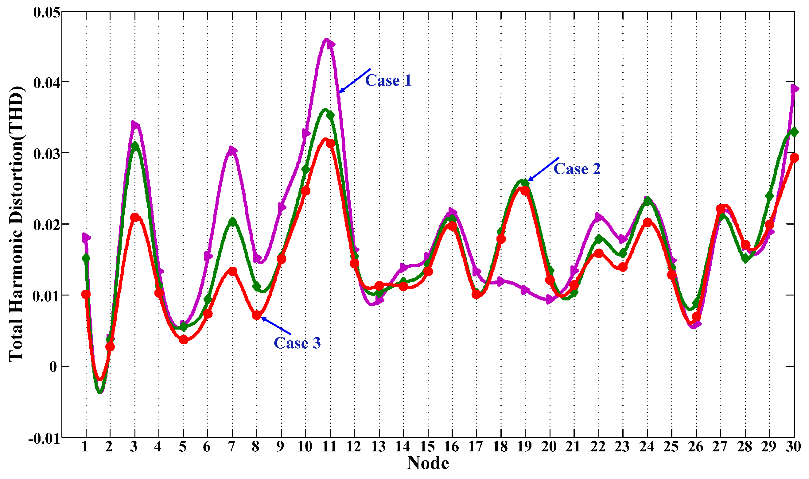
The value of total harmonic distortion (THD) in distribution system with DGs in cases 1–3 is also analyzed. For each installed DGs, the THD of grid-connected current I_grid is supposed as 5% and consist of only second harmonic. As can be seen from Figure 9, the value of THD at each node in case 2 or 3 is largely reduced compared to the value of THD in case 1. This can greatly illustrate that the optimization results in case 2 or 3 is more reasonable than the optimization results in case 1. Besides, the THD profile in case 3 is more excellent than the THD profile in case 2 because more operation risk cost ELIC is considered in case 3.

Voltage unbalance factor (VUF) profiles at each node in cases 1–3 are shown in Figure 10. The value of VUF at each node in case 2 or 3 is largely reduced compared to the value of VUF in case 1. In cases 2 and 3, the value of VUF at each node is less than 2%.

Figure 8. Voltage variations at each node with added DGs in case n.

Figure 8. Voltage variations at each node with added DGs in case n.

Figure 9. THD (total harmonic distortion) at each node with added DGs in case n.

Figure 9. THD (total harmonic distortion) at each node with added DGs in case n.

Figure 10. VUF (Voltage unbalance factor) at each node with added DGs in case n.

Figure 10. VUF (Voltage unbalance factor) at each node with added DGs in case n.

Generally, these simulation results demonstrate that the appropriate siting andsizing of DGs could improve voltage profiles and enhance power-supply reliability and the proposed method for optimal siting and sizing of distributed generators is more reasonable than the traditional method.

7. Conclusions

Expected load interruption cost is used as the assessment of operation risk indistribution systems, which is assessed by point estimate method (PEM). This proposed expected load interruption cost estimationmethod by PEM is slightly low in accuracy, but the computational cost of PEM is largely reduced compared with Monte Carlosimulation.

Combined the costs of system operation planning with expected load interruption cost (ELIC) in distribution systems, a novel mathematical model of chance constrained programming (CCP) framework for optimal siting and sizing of DGs in distribution systems is proposed considering the uncertainties of DGs. Then, a hybrid genetic algorithm (HGA), which combines the genetic algorithm(GA) with traditional optimization methods, is employed to solve the proposed CCP model. This HGA overcome the drawbacks of both GA and traditional optimization methods.

Test results have demonstrated that this proposed CCP model is more reasonable to determine the siting and sizing of DGs compared with traditional CCP model. Simulation results also demonstrate that the appropriate siting andsizing of DGs could lead to many positive effects on the distribution system concerned, such as the reduced total costs associated with DGs, reduced network losses, and improved voltageprofiles and enhanced power-supply reliability.