1. Introduction
Darrieus-type vertical axis wind turbines (DT-VAWTs) are nonlinear systems that operate in turbulent environments. Therefore, it is difficult to accurately characterize their aerodynamic rotor behaviour across a wide range of operating conditions using physically meaningful models. Commonly used models are either derived from wind turbine data and are presented in a “black box” format or are computationally expensive. Indeed, most of these models lack both conciseness and intelligibility and are therefore prohibitive for the routine engineering analyses of the local interaction mechanisms of wind turbines. Furthermore, none of the models with high reliability and accuracy can be efficiently coupled with models of the other mechanical and electrical parts of the wind turbine to form a global model for the wind energy conversion system (WECS).
Models are of central importance in many scientific contexts and are one of the principal instruments of modern science. Scientists spend considerable time building, testing, comparing and revising models, and many scientific publications are dedicated to introducing, applying and interpreting these valuable tools. The use of electrical circuit elements to model physical devices and systems has a long and successful history. Additionally, understanding analogies and constructing an analogue model for a given system allows the system to be studied in an environment other than that for which it is intended [
1,
2,
3], thereby facilitating the study of specific system phenomena. Moreover, a model based on electrical components is accessible and quickly understood by researchers from almost all engineering fields. This wide understanding is of great importance because research and development in the wind turbine industry requires competencies from several different fields of engineering. Furthermore, the equivalent electrical model can take advantage of existing resources by simultaneously capitalizing on the strengths of these resources and minimizing their respective drawbacks. In addition, such a model can be a good tool for simulating wind turbine rotor operation in the case of physical damage or structural faults on one or more blades. Finally, because electrical and other dynamic models for other parts of the wind turbine have been developed [
4,
5,
6,
7,
8,
9,
10,
11], this new rotor model can easily be linked to existing models to create an overall wind turbine model.
This paper presents an electric circuit model for three-blade DT-VAWT rotors that we named the Tchakoua model. This model is based on a recently developed approach for modelling DT-VAWT rotors using the equivalent electrical circuit analogy that is presented in [
12,
13,
14]. The proposed model was built from the mechanical description given by the Paraschivoiu double-multiple streamtube model and was based on an analogy between mechanical and electrical circuits. Thus, the rotating blades and the blades’ mechanical coupling to the shaft are modelled using the mechanical-electrical analogy, and the wind flow is modelled as a source of electric current.
This paper is organized as follows:
Section 2 presents the context of the work and the methodology used for building the model;
Section 3 presents the theoretical background and the model construction; the results are presented and discussed in
Section 4; and
Section 5 concludes the paper.
2. Context and Method
2.1. Context
Due to their compactness, adaptability for domestic installations, omni-directionality, and other advantages, VAWTs have recently become the focus of renewed interest. Several universities and research institutions have conducted extensive research and developed numerous designs based on aerodynamic computational models [
15,
16,
17]. For example, the on-going studies at the University of Québec at Abiti-Témiscamingue could construct a new model that is more appropriate for the design and further conceptual analysis focusing on operational optimization, condition monitoring, and fault prediction and detection of DT-VAWT rotors.
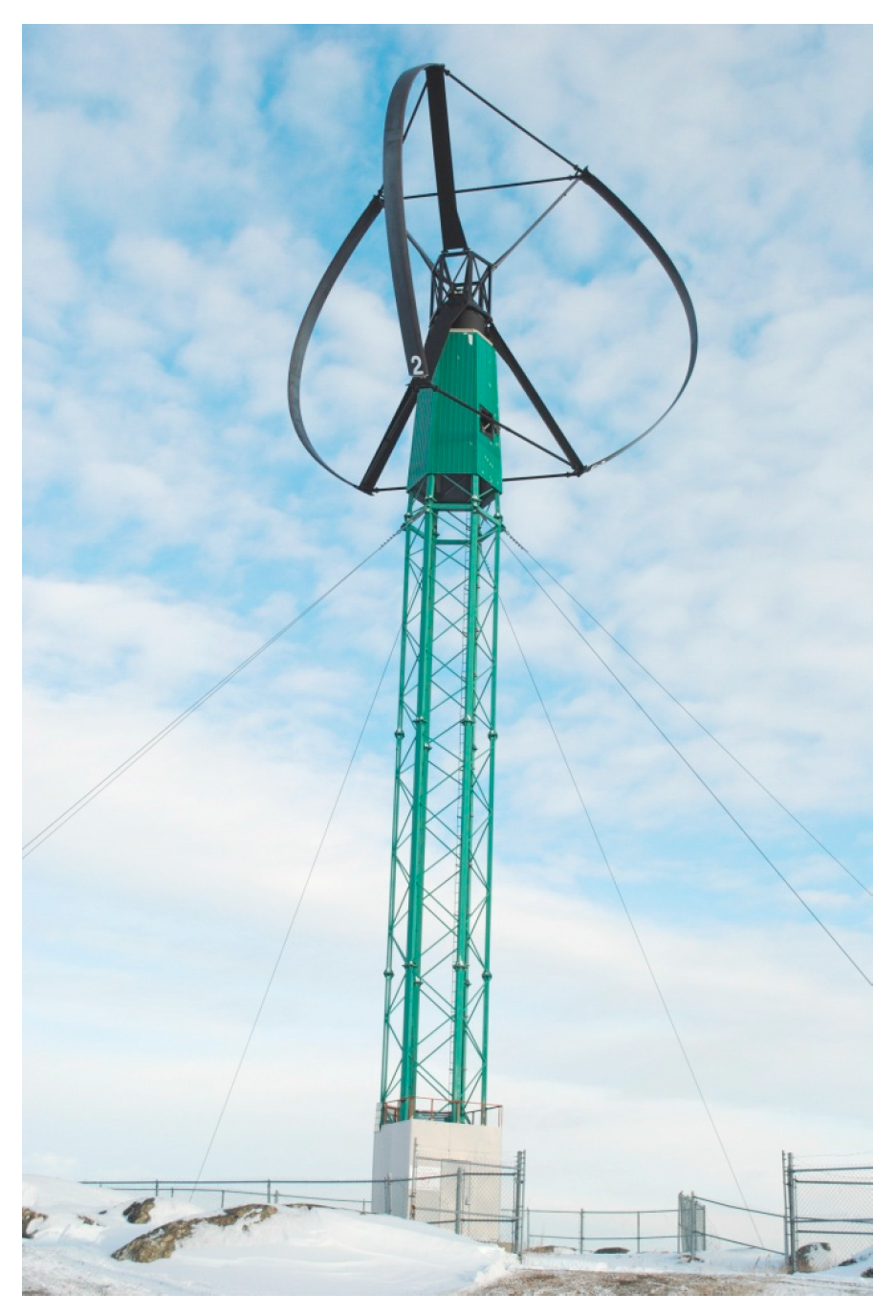
Figure 1 shows the “Cap d’Ours” three-blade VAWT that serves as a teaching and research tool at the University of Québec at Abitibi-Témiscamingue.
Several advances have been made in the understanding and modelling of wind turbine aerodynamics. Various models for VAWT aerodynamic simulation can be found in the literature. These models can be broadly classified into four categories: momentum models, vortex models, cascade models and computational fluid dynamic (CFD) models. A literature survey on the most used models was conducted in [
12,
14]. Aerodynamics are still unable to meet the demands of various applications, although the streamtube and vortex models have seen significant improvements. However, as with all knowledge, our understanding of aerodynamics is not absolute and can be viewed as tentative, approximate, and always subject to revision. For instance, CFD solutions remain very computationally expensive and are prohibitive for routine engineering analyses of the local interaction mechanisms of wind turbines. Furthermore, none of the models with high reliability and accuracy can be efficiently coupled with the models of the other mechanical and electrical parts of the wind turbine to create a global model for the wind energy conversion system (WECS).
To overcome these problems, this paper presents a DT-VAWT model that is built using electric components. The Tchakoua model is a circuit-based model that is advantageous because it allows an electrical engineer to visualize and understand the working principles and the aerodynamics underlying the VAWT rotor functions and behaviour in a connected circuit better than a black box or a complex equation. Indeed, wind energy is a multidisciplinary domain with increasing research in the field of electrical engineering. Furthermore, the Tchakoua model could be linked to existing electric models of other mechanical and electrical parts of a wind turbine to form a global model for the WECS. Such a global circuit-based model for WECS will help users to understand the effects of various parameters on the aerodynamic blade forces and the effects of rotor structural faults on the overall WECS performance. According to [
18,
19,
20], this model will contribute to constructing a global model that can be used to develop or improve the overall condition monitoring technique for WECS. Overall WTCM approaches include performance monitoring, power curve analysis, electrical signature, and supervisory control and data acquisition (SCADA) system data analysis. Compared to subsystem condition monitoring techniques, global system condition monitoring techniques are nonintrusive, low cost and reliable; global monitoring techniques can be used in online monitoring to reduce downtime and OM costs [
21,
22,
23]. Finally, the new model is very versatile and may therefore permit the study of various effects and phenomena, including dynamic stall effects, flow curvature effects, pitching circulation, added mass effects, interference among blades, and vibration effects.
2.2. Method: The Mechanical-Electrical Analogy Approach
Analogies are of greatest use in electromechanical systems when there is a connection between mechanical and electrical parts, especially when the system includes transducers between different energy domains, such as WECS.
Mechanical-electrical analogies are used to represent the function of a mechanical system as an equivalent electrical system by drawing analogies between mechanical and electrical parameters. The main value of analogies lies in the way in which mathematics unifies these diverse fields of engineering into one subject. Tools previously developed for solving problems in one field can be used to solve problems in another field. This is an important concept because some fields, particularly electrical engineering, have developed rich sets of problem-solving tools that are fully applicable to other engineering fields [
24]; for example, there are simple and straightforward analogies between electrical and mechanical systems. Furthermore, analogies between mechanical systems and electrical or fluid systems are effective and commonly used.
Two valid techniques for modelling mechanical systems with electrical systems or for drawing analogies between the two types of systems can be found in the literature, and each method has its own advantages and disadvantages [
25,
26,
27,
28]. The first technique is intuitive; in this technique, current corresponds to velocity (both consist of motion), and voltage corresponds to force (both provide a “push”). The second technique is the through/across analogy that uses voltage as an analogy for velocity and current as an analogy for force. The two schools of thought for modelling mechanical systems with electrical systems are presented in
Table 1. Although both are valid, the through/across analogy results in a counterintuitive definition of impedance [
24,
29,
30]. The universally applied analogy for impedance is that from the intuitive analogy listed in the corresponding section of
Table 1. Therefore, the intuitive analogy is used in the present study.
3. Model Construction
3.1. Theoretical Background
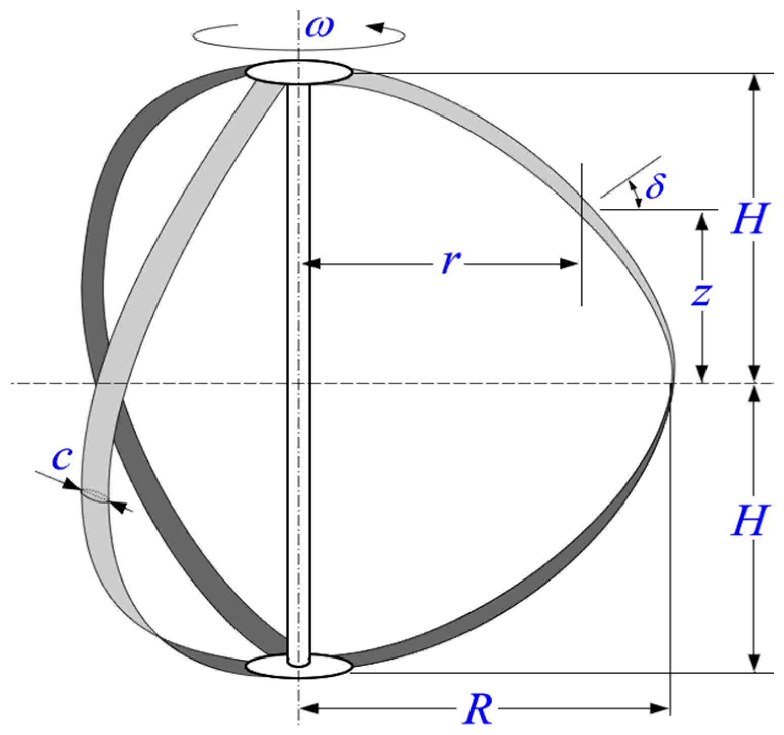
DT-VAWTs are lift-based machines, i.e., their driving torque is mainly generated by the lift force, and they consist of two or more aerofoil-shaped blades attached to a rotating vertical shaft. The interaction between the wind and the rotating blades creates a system of lift and drag forces over the blades themselves. The instantaneous resultant of these forces is dominated by the lift effect that is responsible for the aerodynamically generated mechanical torque. If we consider a Darrieus-type VAWT, as shown in
Figure 2, the aerofoil blade is characterized by the height 2
H, the rotor radius
R, the number of blades
Nb = 3 and the blade chord
c. For a given point on any of the blades,
r and
z are the local radius and height, respectively. When the rotor is subject to an instantaneous incoming wind speed
W0(
t), it turns at a rotational speed ω(
t).
Figure 3 shows the aerodynamic forces and the three velocity vectors acting on DT-VAWT blade elements at a random position [
31,
32].
FL and
FD are the lift and drag force, respectively. As the blade rotates, the local angle of attack α varies with the relative velocity
Wr. The incoming wind speed
W0 and the rotational velocity of the blade ω govern the orientation and magnitude of
Wr [
33,
34]. In turn, the forces
FL and
FD acting on the blade vary. The magnitude and orientation of the lift and drag forces vary along with the resultant force. The resultant force can be decomposed into a normal force
FN and a tangential force
FT. The tangential force component drives the rotation of the wind turbine and produces the torque necessary to generate electricity [
35].
A new approach for modelling DT-VAWT rotors using the electric-mechanic analogy was presented in [
12,
13,
14]. These works provide a proof-of-concept demonstration of the approach and verify the feasibility of such a model through step-by-step demonstrations of the theoretical and practical concepts that underpin the new model as well as simulations and cross-validation of a single-blade model.
3.1.1. Wind Flow as a Current Source
As stated in [
12,
14], an analogy can be made between the wind flow in a streamtube and an electric current. If the incident wind flow is assumed to be an electric current, then the wind’s relative dynamic pressure flow can be defined as
(where
q is given in
and the fluid density
ρ is given in kg/m
3), which is the energy of the wind due to its velocity, that can be considered an electric energy source. Thus, the instantaneous expression of the current source that represents the relative wind seen by the blade is as follows:
where
and
.
is the modulus of the current flow that varies with the rotational angle of the blade. For the Double-multiple multi-streamtube model shown in
Figure 4, the modulus of the corresponding current in the downwind disk is slightly lower than that in the upwind disk (
).
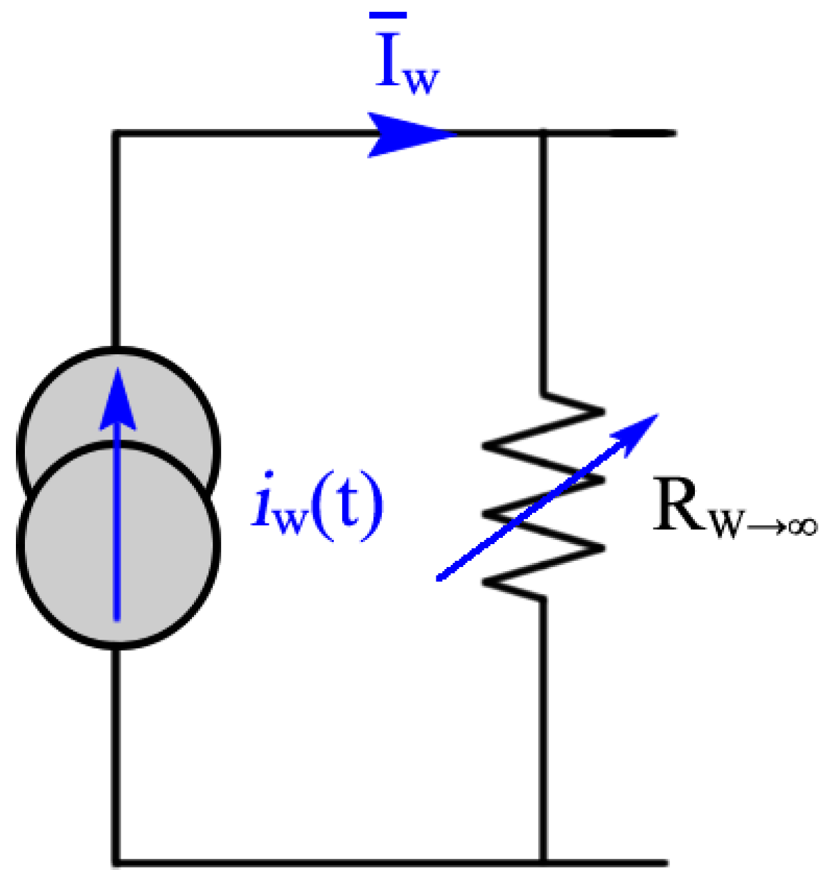
As described in [
12,
14], the airflow in a streamtube can be compared to wind flow on a thin flat disc that is parallel to the airstream. In such conditions, the resistance to the airflow due to air friction on both sides of the plate is minimal, and the wind driving pressure difference from one point of the streamtube to another is approximately zero. Thus, the resistance to wind flow is zero, meaning that the electric resistance parallel to the current source tends to infinity such that the total current produced by the current generator flows in the blade. The improved equivalent electric model for wind flow in a double-multiple multi-streamtube model is shown in
Figure 5.
3.1.2. Electric Circuit Model for a Single Blade
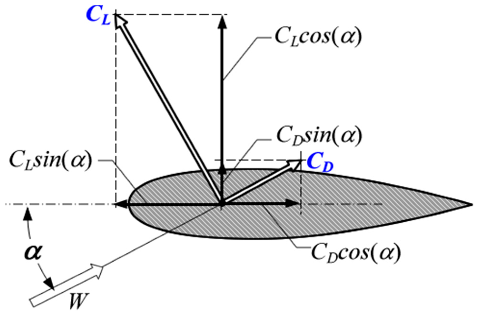
The aerodynamic force coefficients acting on a cross-sectional blade element of a Darrieus wind turbine are shown in
Figure 6. The directions of the lift and drag coefficients as well as their normal and tangential components are illustrated in this figure. The effort variable is voltage, while the flow variable is electrical current. The ratio of voltage to current is the electrical resistance (Ohm’s law). The ratio of the effort variable to the flow variable in other domains is also described as resistance. Oscillating voltages and currents with a phase difference between them provide the concept of electrical impedance. Impedance can be considered an extension to the concept of resistance: resistance is associated with energy dissipation, while impedance encompasses both energy storage and energy dissipation.
We consider a complex coordinate system as shown in
Figure 6, where the vertical axis is assumed to be real and the horizontal axis is assumed to be imaginary. Then, the lift and drag coefficients can be written as follows:
The total impedance for a blade element is obtained by adding the elementary lift and drag impedances. We can then write:
where
and
where
and
are the resistive and inductive components of the lift impedance, respectively, while
and
are the resistive and inductive components of the elementary drag impedance, respectively. Because
varies with the angle of attack α,
and
correspond to a variable resistor (
) and a variable inductor (
), respectively. Similarly, because
varies with the angle of attack α,
and
correspond to a variable resistor (
) and a variable capacitor (
), respectively.
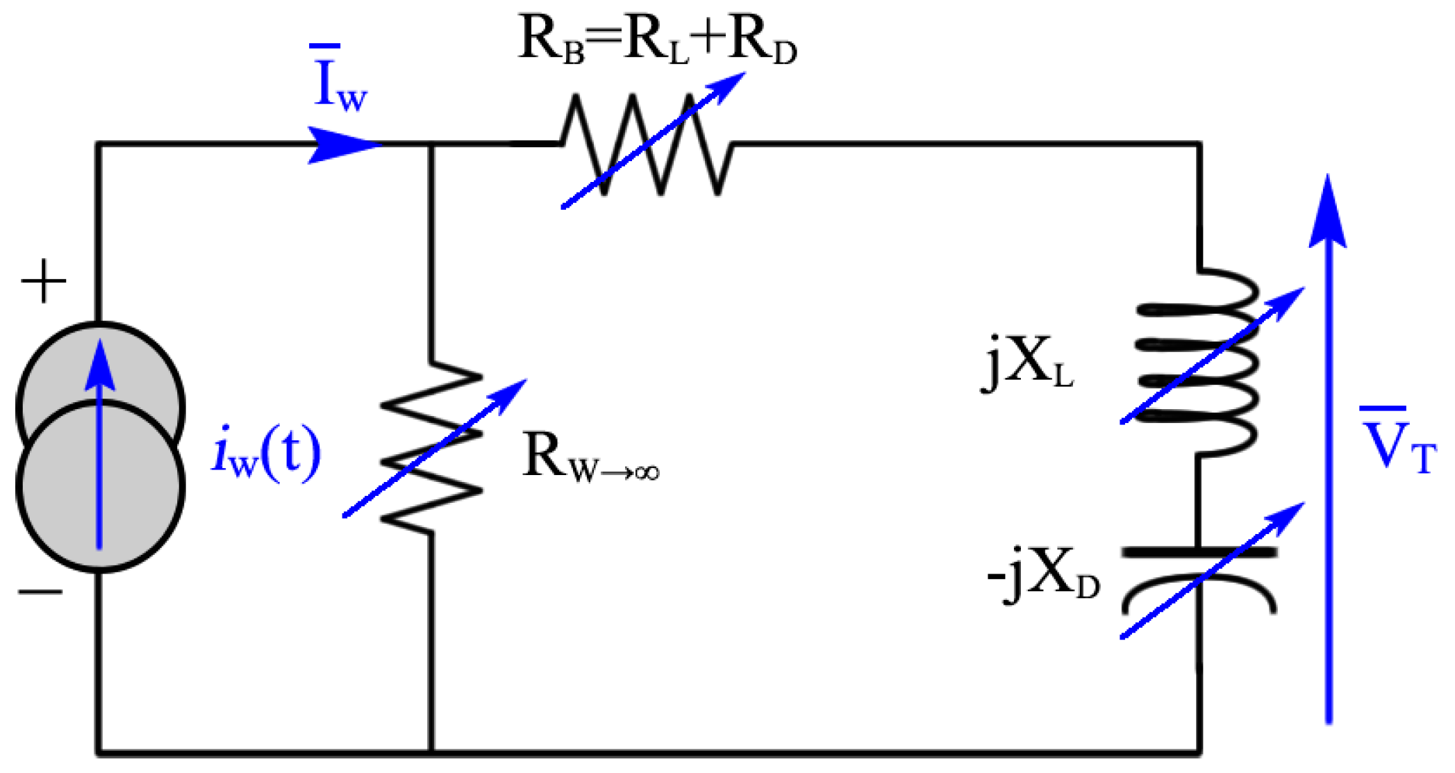
Figure 7 shows the enhanced equivalent electric model of a single blade. The normal and tangential voltages produced by the blade can be expressed as follows:
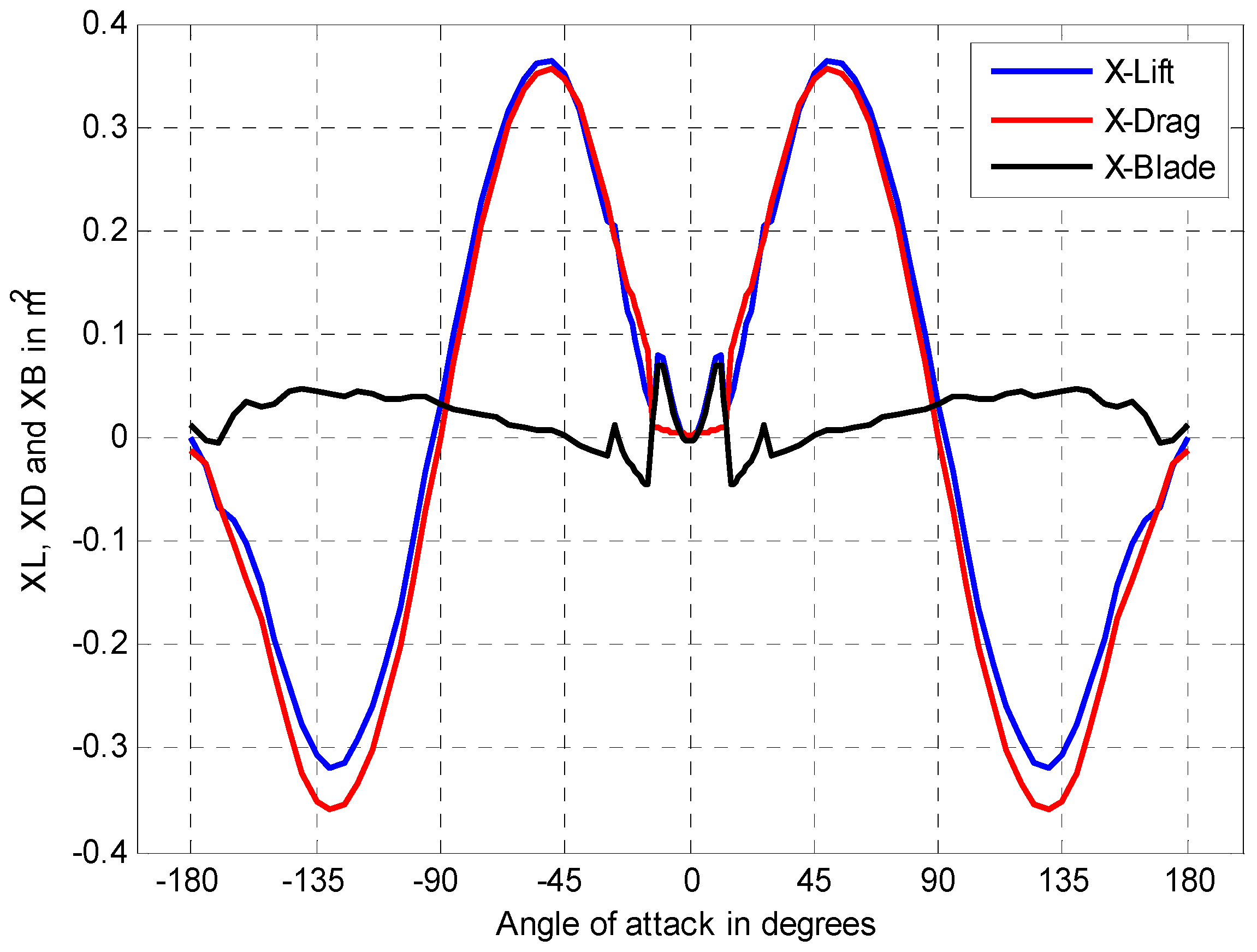
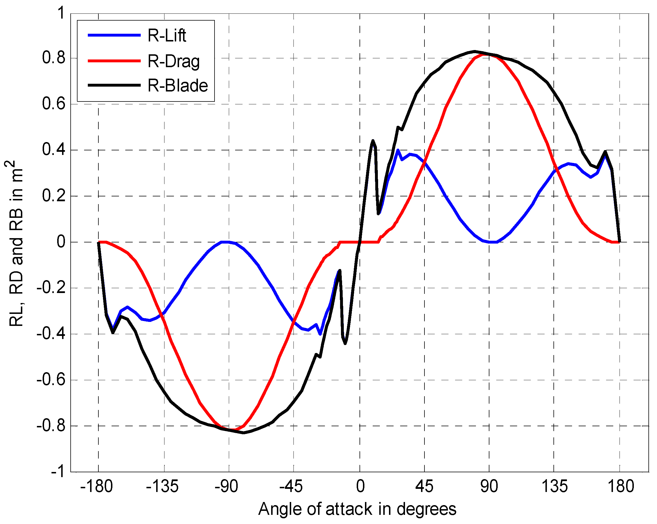
The variation of the lift, drag and normal resistances as well as those of the lift, drag and tangential reactances are shown in
Figure 8 and
Figure 9, respectively [
14]. These resistances and reactances are obtained considering a blade element; therefore, they are given per unit of blade height.
Following the laws of electrical circuit analysis, the branch with
can be assumed to be an open circuit, and the total voltage across a blade can be obtained from the algebraic sum of the lift and drag voltages. We can then write:
When the blade is turning, the elementary work (or elementary amount of mechanical energy) is produced when an elementary force is exerted on an elementary linear distance
covered by the blade. Furthermore, because the torque varies with the azimuth angle of the blade, the torque produced by a blade element is obtained by integrating with respect to the rotational angle. Then, the total torque produced by the entire blade for a complete revolution of the turbine is obtained by adding n discrete elementary torques over the full height of the rotor:
The final expression of the total torque is then obtained;
3.2. Electric Circuit Model for the Blades’ Mechanical Coupling to the Shaft
The wind turbine shaft is connected to the centre of the rotor; this shaft supports the rotor (hub and blades) and transmits the rotary motion and torque moments of the rotor to the gearbox and/or generator. When the rotor spins, the shaft spins as well. In this way, the rotor transfers its rotational mechanical energy to the shaft and then to an electrical generator on the other end. If we assume that the rotor’s mechanical coupling to the shaft is ideal, then it would be electrically equivalent to an ideal transformer.
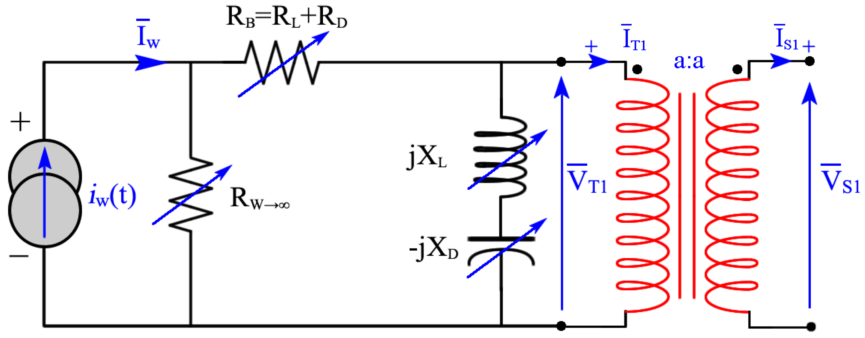
Figure 10 shows the equivalent electric diagram for a single blade coupled to the shaft.
At this stage of the WECS (shaft), we no longer consider fluid mechanics; instead, we address translation and/or rotation mechanics. Assuming an ideal autotransformer, the voltage at the primary side is equal to that at the secondary side, i.e.,
. The current produced by the source corresponds to the relative wind seen by the blades at any moment. That is, for each blade:
where
and
.
Because the mechanical coupling of a single blade
i to the shaft can be modelled as an ideal autotransformer, we can then write:
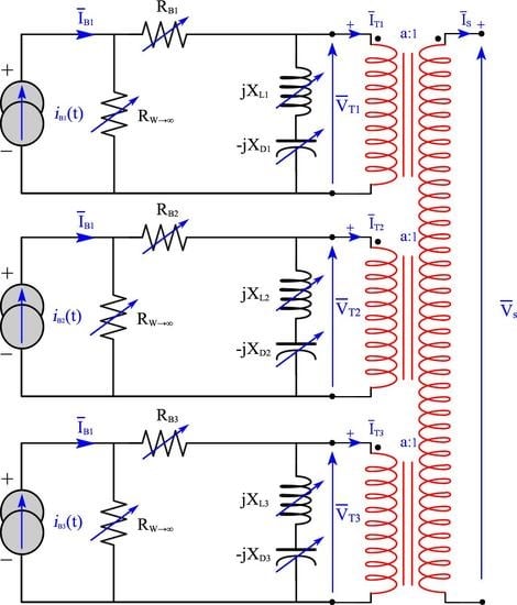
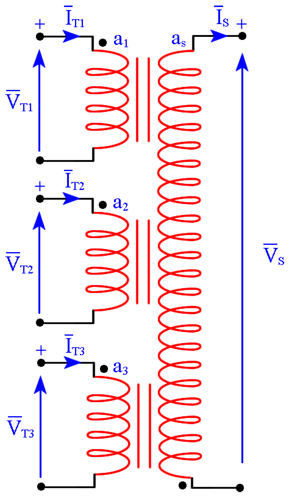
Assuming that the rotor mechanical coupling of three blades to the shaft is ideal, this coupling can be electrically modelled as multiple ideal primary transformers, as shown in
Figure 11.
The windings of the corresponding transformer are made so that the following is true:
Because we have
, we can write:
The voltage at the secondary of the transformer can be obtained by vector addition of the three primary voltages because , and have variable moduli and phases while the phase difference from one blade to another remains constant. At any instant, the three voltages behave as if in an unbalanced three-phase system.
As suggested in the intuitive analogy, the rotational speed of the shaft ω is analogous to the electrical current. Finally, the rotational speed of the shaft can be assumed to be equivalent to the electric current at the secondary of the transformer, i.e.,
IS = ω. We can therefore write the following relations:
4. Results and Discussion
4.1. Electric Circuit Model for Three-Blade DT-VAWT Rotors: The Tchakoua Model
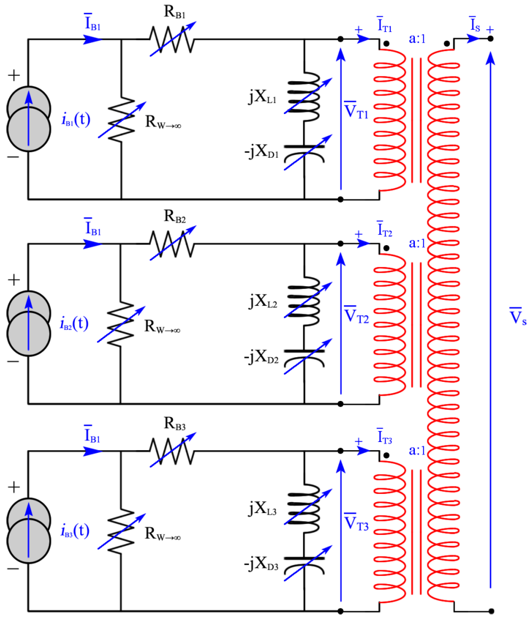
We can now construct the equivalent electric model for the whole three-blade turbine. The equivalent circuits for various blades are brought together and are coupled based on the developments presented in
Section 3.
Figure 12 presents the Tchakoua model, which is the global equivalent electric model for a three-blade DT-VAWT.
Because the rotor has three blades, the angle between two blades is . If we assume a constant wind flow, then the blades are subject to the same current vector with their respective phase delays. Assuming that the rotor turns in the forward rotational direction, we can write:
; and .
Then, the following matrix can be obtained:
Considering the operator
, we have
and
. Thus, the voltage vectors for the three-blade rotor can be written as follows:
Following
Figure 4, the apparent power representing the contribution of the whole rotor to the shaft power can be obtained by adding the power produced by the three blades separately:
The voltage produced by a sectional element of a single blade varies with its azimuth position and relative radius and height. The curved blade is discretized into n blade elements, as suggested in [
14], and the average power produced by a blade element for a complete revolution of the turbine is obtained by integrating the elementary power with respect to θ.
For different blades, the blades elements at the same high will produce the same power. We can then write:
Finally, the total average power produced by sectional element of the rotor is obtained by adding the power from each of the three blades.
4.2. Simulation Results
This section presents the results of the Tchakoua model for a three-blade DT-VAWT. The simulations were performed in MATLAB using data for NACA0012 that was obtained from different literature sources [
37,
38,
39] with Reynolds numbers ranging from 500,000 to approximately 750,000. We choose the NACA0012 blade profile because it is one of the most studied and most commonly used profiles [
39] Finally, the simulation results were assessed using results from the literature [
40].
The simulation characteristics of the rotor were taken from [
34] and are presented in
Table 2.
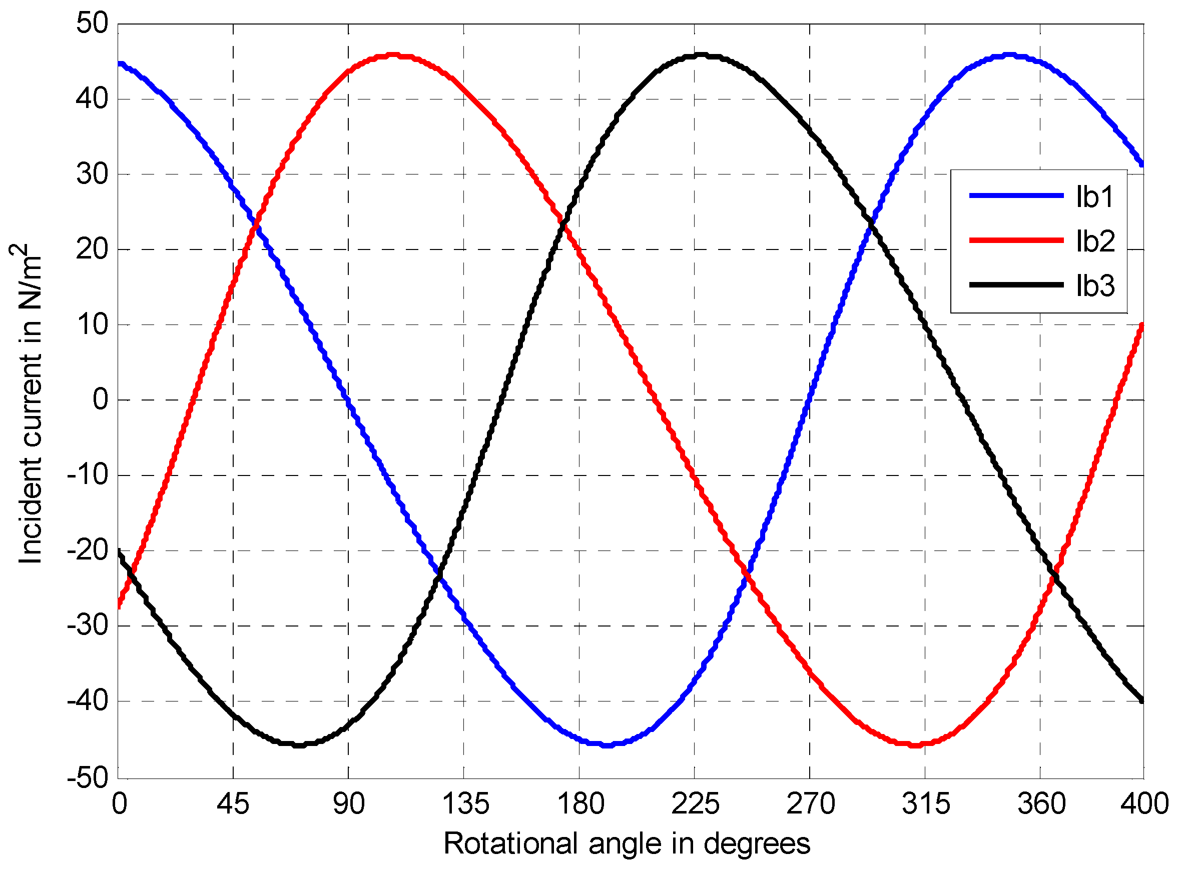
4.2.1. Simulation Results for Current Sources
Figure 13 shows the current variations for each blade. These variations are similar to those of AOA as a function of the rotational angle of the blade. In addition, the incident current for a given blade is at a maximum when its AOA is at a maximum; similarly, the incident current is minimal or zero when the AOA is minimal or zero. Furthermore, the incident currents appear similar to the alternating current of a symmetric three-phase power supply system with the same frequency and voltage amplitudes relative to a common reference but with a phase difference that is one-third of the period.
4.2.2. Variations of the Resistances and Reactances in the Model
The total normal and resistive components of the blade impedance
Rb and the total tangential and reactive components of the blade impedance
Xb are plotted using the relations in Equations (4) and (5).
Figure 14 and
Figure 15 show the variations of
Rb and
Xb for the three blades as functions of the rotational angle.
For a given blade, the resistance is zero when the blade rotational angle corresponds to wind incident angle equal to zero, that is a shortly before and for B1. At these positions, the blade is parallel to the wind flow streamtubes, and the incident angle is therefore zero. In addition, the blade’s B1 resistance is at a maximum when corresponding wind incident angle is minims, which corresponds to a position close to 190° from the reference point for these blade positions, the blades are perpendicular to the wind flow streamtubes, and the incident angle is at its maximum. Furthermore, the resistances vary between positive and negative quantities. According to our model inspired from double-multiple multi-streamtube models, the resistance of the blade to the wind flow is considered to be positive in the upwind disk and negative in the downwind disk.
The reactance of B1 is minimal when it is at and . At these positions, the blade is parallel to the wind flow streamtubes, and the incident angle is therefore zero; thus, the contribution of the wind to the torque production is negligible. Starting from , the blade reactance continue to increase reaching two maximums respectively at 160° and 220°. At between 160° and 220°, a valley appears that is caused by dynamic stall, which occurs when an aerofoil, operating in unsteady flow, overcomes the static stall angle. For a VAWT with a fixed blade geometry in unsteady flow and a given induction factor, the angle of attack is a function of the azimuth angle; for λ < 5, the angle of attack can overcome the static stall angle, causing dynamic stall. During dynamic stall, large leading edge separated vortices are formed, delaying lift loss until they are convected over the surface results in a rapid decrease in lift.
4.2.3. Variations of the Normal and Tangential Voltages
Figure 16 and
Figure 17 plot the normal and tangential voltage variations as functions of the blade position, respectively.
The normal voltage produced by the blade during a complete rotation varies from zero to a minimal value. All the normal voltages are negative quantities at any instant of blade rotation because they stem from the drag coefficient and constitute obstructions to the blade rotation, meaning that they are negative contributions to the torque production. During a complete rotation of the reference blade, there are two minimums at rotational angles for which the angle of attack is zero at 190° and 350°. The negative value of the resistance matches the contribution of this impedance element in the blade movement and thus in the torque production.
The tangential voltage produced by the blade during a complete rotation varies following an alternative and 2π periodic signal. During a complete rotation of the blade, the tangential voltage is equal to zero at
and
; these points are also inflexion points that correspond to angles for which the tangential impedance is zero. Similar to the tangential impedance, a valley occurs between 160° and 220° due to dynamic stall. The total voltage produced by the rotor is obtained by adding the voltages produced by the blades. As shown in
Figure 17, the total voltage is an alternative and
periodic signal is not equal to zero because at any moment, the blade voltage is an unbalanced three-phase system. The effect of dynamic stall can also be observed for the total voltage at
and every
after this point.
4.2.4. Power Variations Produced as a Function of the Rotational Angle
The power produced by individual blades and the total power produced by the whole rotor are plotted in
Figure 18. These results agree with findings in [
32,
35,
41,
42,
43]. The power produced by each blade is always positive and is a variable and periodic quantity with a period of π. The power produced by a blade varies similar to the reactance with negative reactance producing positive power. A phase difference of
exists between the powers of the three blades. The total power for the rotor is always a positive quantity; is variable and periodic with a period of
. The results obtained show strong agreement with results from both aerodynamic and CFD models in the literature.
The normal and tangential voltages are both periodic values that undergo important variations during rotor rotation. The total tangential voltage produces the total torque.
5. Conclusions
In this paper, an electric circuit model for a three-blade DT-VAWT rotor is proposed. The new Tchakoua model is based on a new approach for modelling DT-VAWT rotors using the mechanical-electrical analogy. Indeed, the construction of this novel model is further to the proof-of-concept demonstration of the relevancy of modelling VAWTs rotors using electrical equivalent circuit analogy that was performed in previous research work. The model is based on an analogy with the double multiple streamtube model and was obtained by combining the equivalent electrical models for the wind, the three blades and the mechanical coupling. For validation, simulations were conducted using MATLAB for a three-bladed rotor. Results obtained for models outputs such as voltages and power are consistent with findings of the Paraschivoiu double-multiple streamtube model as well as Frank Scheurich among others.
The Tchakoua model is more appropriate for the design, performance prediction and optimization of Darrieus rotors. Mechanical fault diagnosis and prognosis are also important because the model can be used to simulate rotor behaviour in the event of mechanical faults in one or more of the blades or in the rotor-shaft coupling elements. The model can also simulate turbine operation in the event of mechanical faults in one or more rotor elements. The simulations were conducted in MATLAB, and the results show high accuracy with the Paraschivoiu model as well as other results in the literature.
Despite the very simple design philosophy of VAWTs, their aerodynamics presents several challenges. The main feature of VAWTs is that the effective angle of attack “seen” by the blades undergoes a very large variation that in moderate to low tip speed conditions drives the blades into stall for both negative and the positive angles of attack. In future works, we intend to implement the Tchakoua model in simulation tools such as MATLAB Simulik or P-SPICE to study the effects of varying angles of attack within the post-stall region on flow unsteadiness and dynamic stall phenomena. The model could be extended to other types of wind turbines including horizontal axis wind turbines, Savonious-type VAWTs and hybrid Darrius‑Savonius VAWTs. Additionally, the Tchakoua model will be used to study the influence of wind flow turbulence on turbine vibrations. Transitional (starting) and permanent sate functioning of VAWTs may also be examined. Finally, we intend to use the model to study the impact of structural faults in one or more blades on a DT-VAWT. As a long-term goal, the Tchakoua model will be linked to existing models of other electrical and mechanical wind turbine parts to obtain a global Darrieus-type WECS model.
Acknowledgments
The authors would like to thank the Natural Science and Engineering Research Council of Canada (NSERC) for financially supporting this research. The authors are also grateful to the editor and the four anonymous reviewers for their valuable comments and suggestions that improved the quality of this paper.
Author Contributions
Pierre Tchakoua is the main author of this work. This paper further elaborates on some of the results from his Ph.D. dissertation. René Wamkeue and Mohand Ouhrouche supervised the project and supported Pierre Tchakoua’s research in terms of both scientific and technical expertise. Gabriel Ekemb and Ernesto Benini assisted in the results analysis and interpretation. The manuscript was written by Pierre Tchakoua and was reviewed and revised by René Wamkeue, Mohand Ouhrouche and Ernesto Benini.
Conflicts of Interest
The authors declare no conflicts of interest.
Abbreviations
| Area of a blade element |
| Chord of the blade (m) |
| Equivalent or total coefficient |
| Lift coefficient |
| Drag coefficient |
| Normal coefficient |
| Tangential coefficient |
| Total or equivalent coefficient |
| Normal force (N) |
| Tangential force (N) |
| Lift force (N) |
| Drag force (N) |
| Half of rotor’s height (m) |
| Instantaneous current that represents the incident wind flow |
| Current at the primary side of the transformer |
| Current at the secondary side of the transformer |
| Number of blades |
| Relative dynamic pressure flow (N/m2) |
| Local radius of the blade (m) |
| Drag resistance |
| Lift resistance |
| Resistance to wind flow |
| Reynolds number |
| Rotor radius (m) |
| Apparent power produced by the blade |
| Total apparent power produced by the rotor |
| Blade torque |
| Rotor torque |
| Kinematic viscosity of air (m) |
| Total voltage across the blade |
| Normal voltage across the blade |
| Tangential voltage across the blade |
| Incoming wind speed (m/s) |
| Linear velocity of the blade (m/s) |
| Relative wind speed seen by the blade (m/s) |
| Incident wind on the wind turbine rotor (m/s) (relative wind speed seen by the blade when aligning the blade motion with the negative real axis) |
| Blade shift position |
| Lift reactance |
| Drag reactance |
| Local height of the blade from H (m) |
| Drag impedance |
| Total impedance of the blade |
| Normal impedance of the blade |
| Tangential impedance of the blade |
| Lift impedance |
| Angle of attack or angle of the wind with respect to the X axis |
| Pitch angle of the blade |
| Angle of the relative wind speed (deg) |
| Angle of the blade relative to the vertical axis (deg) |
| Azimuthal angle of the blade |
| Blade tip speed ratio |
| Fluid density (kg/m3) |
| Modulus of the instantaneous current |
| Rotational speed of the rotor (rad/s) |
| CFD | Computational fluid dynamics |
| DT-VAWTs | Darrieus-type vertical axis wind turbines |
| OM | Operations and maintenance |
| SCADA | Supervisory control and data acquisition |
| VAWTs | Vertical axis wind turbines |
| WECS | Wind energy conversion system |
| WTCM | Wind turbine condition monitoring |
References
- Tilmans, H.A. Equivalent circuit representation of electromechanical transducers: I. Lumped-parameter systems. J. Micromech. Microeng. 1996, 6, 157–176. [Google Scholar] [CrossRef]
- Mason, W. An electromechanical representation of a piezoelectric crystal used as a transducer. Proc. Inst. Radio Eng. 1935, 23, 1252–1263. [Google Scholar]
- Tilmans, H.A. Equivalent circuit representation of electromechanical transducers: II. Distributed-parameter systems. J. Micromech. Microeng. 1997, 7, 285–309. [Google Scholar] [CrossRef]
- Barakati, S.M. Modeling and Controller Design of a Wind Energy Conversion System Including a Matrix Converter. Ph.D. Thesis, University of Waterloo, Waterloo, ON, Canada, 2008. [Google Scholar]
- Kim, H.-W.; Kim, S.-S.; Ko, H.-S. Modeling and control of PMSG-based variable-speed wind turbine. Electr. Power Syst. Res. 2010, 80, 46–52. [Google Scholar] [CrossRef]
- Borowy, B.S.; Salameh, Z.M. Dynamic response of a stand-alone wind energy conversion system with battery energy storage to a wind gust. IEEE Trans. Energy Conve. 1997, 12, 73–78. [Google Scholar] [CrossRef]
- Delarue, P.; Bouscayrol, A.; Tounzi, A.; Guillaud, X.; Lancigu, G. Modelling, control and simulation of an overall wind energy conversion system. Renew. Energy 2003, 28, 1169–1185. [Google Scholar] [CrossRef]
- Slootweg, J.; Haan, S.D.; Polinder, H.; Kling, W. General model for representing variable speed wind turbines in power system dynamics simulations. IEEE Trans. Power Syst. 2003, 18, 144–151. [Google Scholar] [CrossRef]
- Junyent-Ferré, A.; Gomis-Bellmunt, O.; Sumper, A.; Sala, M.; Mata, M. Modeling and control of the doubly fed induction generator wind turbine. Simul. Model. Pract. Theory 2010, 18, 1365–1381. [Google Scholar] [CrossRef]
- Bolik, S.M. Modelling and Analysis of Variable Speed Wind Turbines with induction Generator during Grid Fault; Aalborg Universitet: Aalborg, Denmark, 2004. [Google Scholar]
- Perdana, A. Dynamic Models of Wind Turbines; Chalmers University of Technology: Göteborg, Sweden, 2008. [Google Scholar]
- Tchakoua, P.; Ouhrouche, M.; Tameghe, T.A.; Ekemb, G.; Wamkeue, R.; Slaoui-Hasnaoui, F. Basis of theoretical formulations for new approach for modelling darrieus-type vertical axis wind turbine rotors using electrical equivalent circuit analogy. In Proceedings of the 2015 IEEE 3rd International Renewable and Sustainable Energy Conference, Marrakech & Ouarzazate, Morocco, 10–13 December 2015; pp. 1–7.
- Tchakoua, P.; Ouhrouche, M.; Tameghe, T.A.; Ekemb, G.; Wamkeue, R.; Slaoui-Hasnaoui, F. Development of equivalent electric circuit model for darrieus-type vertical axis wind turbine rotor using mechanic-electric analogy approach. In Proceedings of the 2015 IEEE 3rd International Renewable and Sustainable Energy Conference, Marrakech & Ouarzazate, Morocco, 10–13 December 2015; pp. 1–8.
- Tchakoua, P.; Wamkeue, R.; Ouhrouche, M.; Tameghe, T.A.; Ekemb, G. A new approach for modeling Darrieus-type vertical axis wind turbine rotors using electrical equivalent circuit analogy: Basis of theoretical formulations and model development. Energies 2015, 8, 10684–10717. [Google Scholar] [CrossRef]
- Eriksson, S.; Bernhoff, H.; Leijon, M. Evaluation of different turbine concepts for wind power. Renew. Sustain. Energy Rev. 2008, 12, 1419–1434. [Google Scholar] [CrossRef]
- Tjiu, W.; Marnoto, T.; Mat, S.; Ruslan, M.H.; Sopian, K. Darrieus vertical axis wind turbine for power generation I: Assessment of Darrieus VAWT configurations. Renew. Energy 2015, 75, 50–67. [Google Scholar] [CrossRef]
- Bedon, G.; Castelli, M.R.; Benini, E. Optimal spanwise chord and thickness distribution for a Troposkien Darrieus wind turbine. J. Wind Eng. Ind. Aerodyn. 2014, 125, 13–21. [Google Scholar] [CrossRef]
- Tchakoua, P.; Wamkeue, R.; Tameghe, T.A.; Ekemb, G. A review of concepts and methods for wind turbines condition monitoring. In Proceedings of the 2013 IEEE World Congress on Computer and Information Technology (WCCIT), Sousse, Tunisia, 22–24 June 2013; pp. 1–9.
- Tchakoua, P.; Wamkeue, R.; Slaoui-Hasnaoui, F.; Tameghe, T.A.; Ekemb, G. New trends and future challenges for wind turbines condition monitoring. In Proceedings of the 2013 IEEE International Conference on Control, Automation and Information Sciences (ICCAIS), Nha Trang, Vietnam, 25–28 November 2013; pp. 238–245.
- Tchakoua, P.; Wamkeue, R.; Ouhrouche, M.; Slaoui-Hasnaoui, F.; Tameghe, T.A.; Ekemb, G. Wind turbine condition monitoring: State-of-the-art review, new trends, and future challenges. Energies 2014, 7, 2595–2630. [Google Scholar]
- Yang, W.; Tavner, P.J.; Crabtree, C.J.; Wilkinson, M. Cost-effective condition monitoring for wind turbines. IEEE Trans. Ind. Electron. 2010, 57, 263–271. [Google Scholar] [CrossRef] [Green Version]
- Yang, W.; Jiang, J.; Tavner, P.; Crabtree, C. Monitoring wind turbine condition by the approach of Empirical Mode Decomposition. In Proceedings of the 2008 International Conference on Electrical Machines and Systems (ICEMS), Wuhan, China, 17–20 October 2008; pp. 736–740.
- Yang, W.; Tavner, P.; Crabtree, C.; Wilkinson, M. Research on a simple, cheap but globally effective condition monitoring technique for wind turbines. In Proceedings of the 2008 International Conference on Electrical Machines and Systems (ICEMS), Wuhan, China, 17–20 October 2008; pp. 1–5.
- Lewis, J.W. Modeling Engineering Systems: PC-Based Techniques and Design Tools; High Text Publications: San Diego, CA, USA, 1994. [Google Scholar]
- Hogan, N.; Breedveld, P. The physical basis of analogies in network models of physical system dynamics. Simul. Ser. 1999, 31, 96–104. [Google Scholar]
- Olson, H.F. Dynamical Analogies; Van Nostrand: Princeton, NJ, USA, 1958. [Google Scholar]
- Firestone, F. The mobility method of computing the vibration of linear mechanical and acoustical systems: Mechanical-electrical analogies. J. Appl. Phys. 1938, 9, 373–387. [Google Scholar] [CrossRef]
- Calvo, J.A.; Alvarez-Caldas, C.; San, J.L. Analysis of Dynamic Systems Using Bond Graph Method through SIMULINK; InTech: Rijeka, Croatia, 2011. [Google Scholar]
- Firestone, F. A new analogy between mechanical and electrical systems. J. Acoust. Soc. Am. 1933, 4, 249–267. [Google Scholar] [CrossRef]
- Bishop, R.H. Mechatronics: An Introduction; CRC Press: Boca Raton, FL, USA, 2005. [Google Scholar]
- Zhang, L.; Liang, Y.; Liu, X.; Jiao, Q.; Guo, J. Aerodynamic performance prediction of straight-bladed vertical axis wind turbine based on CFD. Adv. Mech. Eng. 2013, 5. [Google Scholar] [CrossRef]
- Paraschivoiu, I. Wind Turbine Design: With Emphasis on Darrieus Concept; Presses Inter Polytechnique: Montreal, QC, Canada, 2002. [Google Scholar]
- Islam, M.; Ting, D.S.-K.; Fartaj, A. Aerodynamic models for Darrieus-type straight-bladed vertical axis wind turbines. Renew. Sustain. Energy Rev. 2008, 12, 1087–1109. [Google Scholar] [CrossRef]
- Scheurich, F.; Fletcher, T.M.; Brown, R.E. Simulating the aerodynamic performance and wake dynamics of a vertical-axis wind turbine. Wind Energy 2011, 14, 159–177. [Google Scholar] [CrossRef] [Green Version]
- Beri, H.; Yao, Y. Double multiple streamtube model and numerical analysis of vertical axis wind turbine. Energy Power Eng. 2011, 3, 262–270. [Google Scholar] [CrossRef]
- Claessens, M.C. The Design and Testing of Airfoils for Application in Small Vertical Axis Wind Turbines. Master’s Thesis, Delft University of Technology, Delft, The Netherlands, 2006. [Google Scholar]
- Sheldahl, R.E.; Klimas, P.C. Aerodynamic Characteristics of seven Symmetrical Airfoil Sections through 180-Degree Angle of Attack for Use in Aerodynamic Analysis of Vertical Axis Wind Turbines; Technical Report; Sandia National Labs: Albuquerque, NM, USA, 1981.
- Critzos, C.C.; Heyson, H.H.; Boswinkle, R.W. Aerodynamic Characteristics of NACA 0012 Airfoil Section at Angles of Attack from 0 to 180 Degrees; National Advisory Committee for Aeronautics: Washington, DC, USA, 1955.
- Miley, S.J. A Catalog of Low Reynolds Number Airfoil Data for Wind Turbine Applications; National Technical Information Service: Alexandria, VA, USA, 1982.
- Timmer, W. Aerodynamic Characteristics of Wind Turbine Blade Airfoils at High Angles-of-Attack; European Wind Energy Association: Brussels, Belgium, 2010. [Google Scholar]
- Li, S.; Li, Y. Numerical study on the performance effect of solidity on the straight-bladed vertical axis wind turbine. In Proceedings of the 2010 Asia-Pacific Power and Energy Engineering Conference (APPEEC), Chengdu, China, 28–31 March 2010; pp. 1–4.
- Attia, E.; Saber, H.; Gamal, H.E. Analysis of straight bladed vertical axis wind turbine. Int. J. Eng. Res. Technol. 2015, 4. [Google Scholar] [CrossRef]
- Scheurich, F.; Brown, R.E. Modelling the aerodynamics of vertical-axis wind turbines in unsteady wind conditions. Wind Energy 2013, 16, 91–107. [Google Scholar] [CrossRef] [Green Version]
Figure 1.
“Cap d’Ours wind turbine”, a curved, three-blade, Darrieus-type VAWT.
Figure 1.
“Cap d’Ours wind turbine”, a curved, three-blade, Darrieus-type VAWT.
Figure 2.
Schematic of a curved, three-blade DT-VAWT.
Figure 2.
Schematic of a curved, three-blade DT-VAWT.
Figure 3.
Velocity and force components for a DT-VAWT.
Figure 3.
Velocity and force components for a DT-VAWT.
Figure 4.
Double-multiple multi-streamtube model.
Figure 4.
Double-multiple multi-streamtube model.
Figure 5.
Electric circuit model for wind flow.
Figure 5.
Electric circuit model for wind flow.
Figure 6.
Aerodynamic coefficients acting on a Darrieus wind turbine blade element [
36].
Figure 6.
Aerodynamic coefficients acting on a Darrieus wind turbine blade element [
36].
Figure 7.
Electric circuit model for a single blade.
Figure 7.
Electric circuit model for a single blade.
Figure 8.
Lift, drag and normal resistance variations as functions of the angle of attack.
Figure 8.
Lift, drag and normal resistance variations as functions of the angle of attack.
Figure 9.
Lift, drag and tangential reactance variations as functions of the angle of attack.
Figure 9.
Lift, drag and tangential reactance variations as functions of the angle of attack.
Figure 10.
Equivalent diagram for a single blade coupled to the shaft.
Figure 10.
Equivalent diagram for a single blade coupled to the shaft.
Figure 11.
Rotor coupling of three blades modelled as an electric transformer.
Figure 11.
Rotor coupling of three blades modelled as an electric transformer.
Figure 12.
Equivalent electric diagram for a three-blade DT-VAWT.
Figure 12.
Equivalent electric diagram for a three-blade DT-VAWT.
Figure 13.
Incident current variations as functions of the rotational angle.
Figure 13.
Incident current variations as functions of the rotational angle.
Figure 14.
Variations of the blade total resistance as a function of the rotational angle.
Figure 14.
Variations of the blade total resistance as a function of the rotational angle.
Figure 15.
Variations of the blade reactance as a function of the rotational angle.
Figure 15.
Variations of the blade reactance as a function of the rotational angle.
Figure 16.
Normal voltage variations of the blade as a function of the rotational angle.
Figure 16.
Normal voltage variations of the blade as a function of the rotational angle.
Figure 17.
Tangential voltage variations of the blades as a function of the rotational angle.
Figure 17.
Tangential voltage variations of the blades as a function of the rotational angle.
Figure 18.
Power produced by the blades as a function of the rotational angle.
Figure 18.
Power produced by the blades as a function of the rotational angle.
Table 1.
System analogy used for developing the new model.
Table 1.
System analogy used for developing the new model.
| Topology-Preserving Set (Book’s Analogy) | |
|---|
| | | | Intuitive Analogy Set |
|---|
| | | ⟸⟹ Intuitive Stretch | | ⟸⟹ Topology Change | | |
|---|
| Description | Trans Mech | Rot Mech | Electrical | Thermal | Fluid | Trans Mech | Rot Mech | Description |
|---|
| “Through” variable | (force) | (torque) | (current) | (heat flux) | q (flow) | (velocity) | ω (angular velocity) | Motion |
| “Across” variable | (velocity) | ω (angular velocity) | ν (voltage) | T, θ | p (pressure) | (force) | (torque) | Push (force) |
| Dissipative element | | | | | | | | Dissipative element |
| Dissipation | | | | N/A | | | | Dissipation |
| Through-variable storage element | or | or | | N/A | | (one end must be “grounded”) | (one end must be “grounded”) | Motion storage element |
| Energy | | | | | | | | Energy |
| Impedance | Standard definition is shown to the right | | | | | | Impedance |
| Across-variable storage element | (one end must be “grounded”) | | | (one end must be “grounded”) | (one end is usually “grounded”) | or | or | Push (force) storage element |
| Energy | | | | (not analogous) | | | | Energy |
| Impedance | The standard definition of mechanical impedance is the one on the right, based on the intuitive analogy | | | | | | Impedance |
Table 2.
Blade simulation characteristics.
Table 2.
Blade simulation characteristics.
| Number of Blades | 3 |
|---|
| Aerofoil section | NACA0012 |
| Blade’s average Reynolds number | 40,000 |
| Aerofoil chord length | 9.14 cm |
| Rotor tip speed | 45.7 cm/s |
| Tip speed ratio | 5 |
| Chord-to-radius ratio | 0.15 |
© 2016 by the authors; licensee MDPI, Basel, Switzerland. This article is an open access article distributed under the terms and conditions of the Creative Commons Attribution (CC-BY) license (http://creativecommons.org/licenses/by/4.0/).


