Short-Term Load Forecasting Based on Wavelet Transform and Least Squares Support Vector Machine Optimized by Improved Cuckoo Search

Abstract

Due to the electricity market deregulation and integration of renewable resources, electrical load forecasting is becoming increasingly important for the Chinese government in recent years. The electric load cannot be exactly predicted only by a single model, because the short-term electric load is disturbed by several external factors, leading to the characteristics of volatility and instability. To end this, this paper proposes a hybrid model based on wavelet transform (WT) and least squares support vector machine (LSSVM), which is optimized by an improved cuckoo search (CS). To improve the accuracy of prediction, the WT is used to eliminate the high frequency components of the previous day’s load data. Additional, the Gauss disturbance is applied to the process of establishing new solutions based on CS to improve the convergence speed and search ability. Finally, the parameters of the LSSVM model are optimized by using the improved cuckoo search. According to the research outcome, the result of the implementation demonstrates that the hybrid model can be used in the short-term forecasting of the power system.

1. Introduction

As an important part of the management modernization of electric power systems, power load forecasting has attracted increasing attention from academics and practitioners. Power load forecasting with high precision can ease the contradiction between power supply and demand and provide a solid foundation for the stability and reliable of the power grid. However, electric load is a random non-stationary series, which is influenced by a number of factors, including economic factors, time, day, season, weather and random effects, which lead to load forecasting being a challenging subject of inquiry [1].

At present, the methods for load forecasting can be divided into two parts: classical mathematical statistical methods and approaches based on artificial intelligence. Most load forecasting theories are based on time series analysis and auto-regression models, including the vector auto-regression model (VAR) [2,3], the autoregressive moving average model (ARMA) [4,5,6], and so on. Time series smoothness prediction methods are criticized by researchers for their weakness of non-linear fitting capability. With the development of the electricity market, the requirement of high accuracy load forecasting is more and more strict and efficient. Therefore, artificial intelligence, which includes neural network and support vector machine, gains increasing attention by scholars. Nahi Kandil and Rene Wamkeue et al. [7] applied short-term load forecasting using the artificial neural network (ANN). The examples with real data showed the effectiveness of the proposed techniques by demonstrating that using ANN can reduce load forecasting errors, compared to various existing techniques. Feng Yu and Xiaozhong Xu [8] proposed an appropriate combinational approach, which was based on an improved back propagation neural network for short-term gas load forecasting, and the network was optimized by the real-coded genetic algorithm. D.K. Chaturvedi et al. [9] applied an algorithm that integrated wavelet transform, the adaptive genetic algorithm and a fuzzy system with a generalized neural network (GNN) to solve the short-term weekday electrical load problem. Luis Hernandez [10] presented an electric load forecast architectural model based on an ANN that performed short-term load forecasting. Nima Amjady and Farshid Keynia [11] proposed a neural network, which was optimized by a new modified harmony search technique. Pan Duan et al. [12] presented a new combined method for the short-term load forecasting of electric power systems based on the fuzzy c-means (FCM) clustering, particle swarm optimization (PSO) and support vector regression (SVR) techniques. Abdollah Kavousi-Fard, Haidar Samet and Fatemeh Marzbani [13] proposed a hybrid prediction algorithm comprised of SVR and modified firefly algorithm, and the experimental results affirmed that the proposed algorithm outperforms other techniques.

The support vector machine (SVM) [14] uses the structural risk minimization principle to convert the solution process into a convex quadratic programming problem. This overcomes some shortcomings in neural networks and has achieved a good performance in practical load forecasting [15]. The problem of hyperplane parameter selection in SVM leads to a large solving scale. In order to solve this, J.A.K. Suykens and J. Vandewalle proposed least squares support vector machine (LSSVM) as a classifier in 1999. Unlike the inequality constraints introduced in the standard SVM, LSSVM proposed equality constraints in the formulation [16]. This results in the solution being transformed from one of solving a quadratic program to a set of linear equations known as the linear Karush–Kuhn–Tucker (KKT) systems [17]. Sun Wei and Liang Yi have applied the method of LSSVM in several engineering problems, including power load forecasting [18], wind speed forecasting [19], project evaluation [20] and carbon emission prediction [21]. For example, in [18], a differential evolution algorithm-based least squares support vector regression method is proposed, and the average forecasting error is less than 1.6%, which shows better accuracy and stability than the traditional LSSVR and support vector regression. The kernel parameter and penalty factor highly effect the learning and generalization ability of LSSVM, and inappropriate parameter selection may lead to the limitation of the performance of LSSVM. However, it is possible to employ an optimization algorithm to obtain an appropriate parameter combination. The particle swarm optimization model [22] and genetic algorithm model [23] model are proposed in parameter optimization for LSSVM. In order to improve the forecasting accuracy of LSSVM, this paper applies the cuckoo search algorithm based on Gauss disturbance to optimize the parameters of LSSVM. Cuckoo search (CS) was proposed by Xin-She Yang and Suash Deb in 2009. CS is a population-based algorithm inspired by the brood parasitism of cuckoo species. It has a more efficient randomization property (with the use of Levy flight) and requires fewer parameters (population size and discovery probability only) than other optimization methods [24]. The advantage of CS is that it does not have many parameters for tuning. Evidence showed that the generated results were independent of the value of the tuning parameters. At present, the CS has been applied in many fields, such as system reliability optimization [25], optimization of biodiesel engine performance [26], load frequency control [27], solar radiation forecasting [28], and so on. In order to improve the convergence speed and the global search ability, the CS algorithm based on Gauss disturbance (GCS) is proposed in which we add Gauss perturbation to the position of the nest during the iterative process. It can increase the vitality of the change of the nest position, thus improving the convergence speed and search ability effectively.

The wavelet transform (WT) is a recently-developed mathematical tool for signal analysis [29,30]. It has been successfully applied in astronomy, data compression, signal and image processing, earthquake prediction and other fields [31]. The combination of WT and LSSVM is widely used in forecasting fields [32,33]. For example, H. Shayeghi and A. Ghasemi [33] introduce WT and improved LSSVM to predict electricity prices. The simulation results show that this technique increases electricity price market forecasting accuracy compared to the other classical and heretical methods in scientific research. Thus, this paper proposes a hybrid model based on WT and LSSVM, which is optimized by GCS, defined as W-GCS-LSSVM, and the examples demonstrate the effectiveness of the model.

The rest of the paper is organized as follows: Section 2 provides some basic theoretical aspects of WT, LSSVM and CS and gives a brief description about the W-GCS-LSSVM model; in Section 3, an experiment study is put forward to prove the efficiency of the proposed model; Section 4 is the conclusion of this paper.

2. W-GCS-LSSVM

2.1. Wavelet Transform

As an effective method for signal processing, the wavelet transform can be divided into two classifications: discrete wavelet transform (DWT) and continuous wavelet transform (CWT). The CWT of a signal $X\left(t\right)$ is defined as follows:

$$CW{T}_{\psi }\left(a,b\right)=\left(1/\sqrt{\left|a\right|}\right){\displaystyle {\int }_{-\infty }^{\infty }x\left(t\right){\psi }^{\ast }\left(\left(t-b\right)/a\right)dt}$$

(1)

where $a$ and $b$ are the scale and the translation parameters, respectively. The equation applied for the DWT of a signal is as follows:

$$DW{T}_x(\mathrm{m},\mathrm{n})=(1/\sqrt{2^m}){\displaystyle \sum _k{x}_k{\psi }^{\ast }((\mathrm{k}-\mathrm{n})/2^m)}$$

(2)

in which m is the scale factor, n = 1, 2...N is the sampling time and N is the number of samples.

As with other WTs, DWT is a kind of WT for which the wavelets are discretely sampled, and it captures both frequency and location information in temporal resolution; thus, DWT has a key advantage over Fourier transforms. In this paper, DWT is used in the data filtering stage.

In WT, a signal is similarly broken up into wavelets, which are the approximation component and detail components, in which the approximation component contains the low-frequency information (the most important part to give the signal its identity) and the detail components to reveal the flavor of the signal. Figure 1 shows a wavelet decomposition process. Firstly, the signal S is decomposed into an approximation component A1 and a detail component D1; then A1 is further decomposed into another approximation component A2 and a detail component D2 in order to meet higher level resolution; and so on, until it reaches a suitable number of levels.

The original short-term load data are proposed to be decomposed into one approximation component and multiple detail components. The main fluctuation of the short-term load data and the details to contain the spikes and stochastic volatilities on different levels are presented in approximation. A suitable number of levels can be decided by comparing the similarity between the approximation and the original signal.

2.2. Least Squares Support Vector Machine

As an extension of the standard support vector machine (SVM), the least squares support vector machine (LSSVM) is proposed by SuyKens and Vandewalle [34]. By transforming the inequality constraints of traditional SVM into equality constraints, LSSVM considers the sum squares error loss function as the loss experience of the training set, which transforms solving the quadratic programming problems into solving linear equations problems [35]. The training set is set as $\{(x_k,y_k)|k=1,2,\mathrm{...},n\}$, in which $x_k\in R^n$ and $y_k\in R^n$ represent the input data and the output data, respectively. $\varphi (•)$ is the nonlinear mapping function, which transfers the samples into a much higher dimensional feature space $\varphi (x_k)$. Establish the optimal decision function in the high-dimensional feature space:

$$y(x)={\omega }^T\cdot \varphi (x)+b$$

(3)

where $\varphi (x)$ is the mapping function; $\omega$ is the weight vector; $b$ is constant.

Using the principle of structural risk minimization, the objective optimization function is shown as follows:

$$\underset{\omega ,b,e}{\min }(\omega ,e)=\frac{1}{2}{\omega }^T\omega +\frac{1}{2}\gamma {\displaystyle \sum _{k=1}^n{e}_k^2}$$

(4)

Its constraint condition is:

$$y_k={\omega }^T\varphi (x_k)+b+e_k k=1,2,\mathrm{...},n$$

(5)

In which $\gamma$ is the penalty coefficient and $e_k$ represents regression error. The Lagrange method is used to solve the optimization problem; the constrained optimization problem can be transformed into an unconstrained optimization problem; the function in the dual space can be obtained as:

$$L(\omega ,b,e,\alpha )=\phi (\omega ,e)-{\displaystyle \sum _{k=1}^n\{{\alpha }_k}[{\omega }^T\varphi (x_k)+b+e_k-y_k]\}$$

(6)

where the Lagrange multiplier ${\alpha }_k\in R$. According to the Karush–Kuhn–Tucker (KKT) conditions, $\omega ,b,e_k,{\alpha }_k$ are taken as partial derivatives and required to be zero.

$$\{\begin{array}{l}\omega ={\displaystyle \sum _{k=1}^n{\alpha }_k\varphi (x_k)}\\ {\displaystyle \sum _{k=1}^n{\alpha }_k=0}\\ {\alpha }_k=e_k\gamma \\ {\omega }^T\varphi (x_k)+b+e_k-y_k=0\end{array}$$

(7)

According to Equation (7), the optimization problem can be transformed into solving a linear problem, which is shown as follows:

$$\left[\begin{array}{cccc}0& 1& \dots & 1\\ 1& K(x_1,x_1)+\frac{1}{\gamma }& \cdots & K(x_1,x_l)\\ ⋮& ⋮& ⋮& ⋮\\ 1& K(x_l,x_1)& \cdots & K(x_l,x_l)+\frac{1}{\gamma }\end{array}\right]\left[\begin{array}{c}b\\ {\alpha }_1\\ ⋮\\ {\alpha }_l\end{array}\right]=\left[\begin{array}{c}0\\ y_1\\ ⋮\\ y_l\end{array}\right]$$

(8)

Solve Equation (8) to get $\alpha$ and $b$, then the LSSVM optimal linear regression function is:

$$f(x)={\displaystyle \sum _{k=1}^l{\alpha }_k}K(x,x_k)+b$$

(9)

According to the Mercer condition, $K(x,x_i)=\varphi {(x)}^T\cdot \varphi (x_l)$ is the kernel function. In this paper, set the radial basis function (RBF) as the kernel function, which is shown in Equation (10):

$$K(x,x_k)=\exp (-\frac{{\left|x-x_k\right|}^2}{2{\sigma }^2})$$

(10)

In which ${\sigma }^2$ is the width of the kernel function.

From the problems of training the LSSVM, kernel parameter ${\sigma }^2$ and penalty parameter $\gamma$ are generally set based on experience, which leads to the existence of randomness and inaccuracy in the application of the LSSVM algorithm. To solve the problem, the paper applies GCS to optimize these two parameters to improve the prediction accuracy of LSSVM.

2.3. Cuckoo Search

The cuckoo search (CS) algorithm is a new optimization metaheuristic algorithm [24], which is on the basis of the stochastic global search and the obligate brood-parasitic behavior of cuckoos by laying their eggs in the nests of host birds. In this optimization algorithm, each nest represents a potential solution. The cuckoo birds choose recently-spawned nests, so that they can be sure that eggs could hatch first because a cuckoo egg usually hatches earlier than its host bird. In addition, by mimicking the host chicks, a cuckoo chick can deceive the host bird to grab more food resources. If the host birds discover that an alien cuckoo egg has been laid (with the probability $p_a$), they either propel the egg or abandon the nest and completely build a new nest in a new location. New eggs (solutions) laid by the cuckoo choose the nest by Levy flights around the current best solutions. Additionally, with the Levy flight behavior, the cuckoo speeds up the local search efficiency.

Yang and Deb simplified the cuckoo parasitic breeding process by the following three idealized rules [24]:

(i)

Each cuckoo lays only one egg at a time and randomly searches for a nest in which to lay it.

(ii)

An egg of high quality will be considered to survive to the next generation.

(iii)

The number of available host nests is fixed, and a host can discover an alien egg with a probability $p_a\in [0,1]$. In this case, the host bird can either throw the egg away or abandon the nest so as to build a completely new nest in a new location. The last strategy is approximated by a fraction $p_a$ of the n nests being replaced by new nests (with new random solutions at new locations).

In sum, two search capabilities have been used in cuckoo search: global search (diversification) and local search (intensification), controlled by a switching/discovery probability ($p_a$). Local search can be described as follows:

$$x_i^{(t+1)}=x_i^t+\alpha s\oplus H(p_a-\epsilon )\otimes (x_j^t-x_k^t)$$

(11)

where $x_j^t$ and $x_k^t$ are different random sequences; $H(u)$ is the Hedwig–Cede function; $\epsilon$ represents a random number; $s$ means the step lengths. The global search is based on Levy flight, which is shown as follows:

$$x_i^{(t+1)}=x_i^t+\alpha \oplus L(s,\lambda )$$

(12)

where $L(s,\lambda )=\frac{\lambda \mathsf{\Gamma }(\lambda )\sin (\pi \lambda /2)}{\pi }\frac{1}{s^{1+\lambda }}, s>>s_0, 1<\lambda \le 3$; $\alpha$ is the levy flight step size multiplication processes with an entry-wise multiplication process. The product $\oplus$ means entry-wise multiplications, which is similar to those used in PSO, but the random walk process via Levy flight here is more efficient in exploring the search space, for its step length is much longer in the long run. It is worth pointing out that, in the real world, if a cuckoo’s egg is very similar to a host’s eggs, then this cuckoo’s egg is less likely to be discovered; thus, the fitness should be related to the difference in solutions. Therefore, it is a good idea to do a random walk in a biased way with some random step size location [36].

The pseudo-code for the CS is performed in Figure 2:

2.4. CS Algorithm Based on Gauss Disturbance

On the basis of the cuckoo search algorithm (CS), the CS algorithm based on the Gauss disturbance (GCS) is proposed in which we add Gauss perturbation to the position of the nest during the iterative process. It can increase the vitality of the change of the nest position, thus improving the convergence speed and search ability effectively.

The basic idea of the cuckoo search algorithm (CS) based on Gauss perturbation is: continue to conduct the Gauss perturbation of $x_i^t$ to make a further search instead of coming directly into the next iteration when a better set of nest locations $x_i^t,i=1,2,\mathrm{...},n$ is gained after t iterations in CS. Suppose $x_i^t,i=1,2,\mathrm{...},n$ is a d-dimensional vector and $p_t$ is described as $p_t={[x_1^{(t)},x_2^{(t)},\mathrm{...},x_n^{(t)}]}^T$, then $p_t$ is a $d\times n$ matrix. The specific operation of GCS algorithm is adding Gauss perturbation to $p_t$, namely:

$$p_t^{\prime }=p_t+a\oplus \epsilon$$

(13)

where $\epsilon$ is a random matrix of the same order to $p_t$, ${\epsilon }_{ij}~N(0,1)$; $a$ is a constant; $\oplus$ represents the point-to-point multiplication. The large range of the value of $\epsilon$ easily leads to the large deviation of the nest location. Therefore, we select $a=1/3$ to control the search scope of $\epsilon$, thus moderately increasing the vitality of the change of the nest position to make $p_t^{\prime }$ reasonable. Then, compare it with each nest in $p_t$ and update $p_t^{″}$ with a better set of nest positions. For the next iteration, $p_t^{″}$ can be represented as $p_t={[x_1^{(t)},x_2^{(t)},\mathrm{...},x_n^{(t)}]}^T$.

2.5. LSSVM Optimized by the CS Algorithm Based on Gauss Disturbance

The flowchart of the W-GCS-LSSVM model is shown in Figure 3, and the detailed processes are as follows:

(1) Decompose the load signal into the approximation A1 and the details D1, and select A1 as the training data and testing data. Normalize the load data.

(2) Determine the value range of ${\sigma }^2$ and $\gamma$ of LSSVM and related parameters of GCS. In this paper, the number of host nests is 25; the maximum number of iterations is 400; and the search range is between 0.01 and 100.

(3) Suppose the initial probability parameter $p_a$ is 0.25, and set $p_i^0={[x_1^0,x_2^0,\mathrm{...},x_n^0]}^T$ as the location of a random n nest. Each nest corresponds to a set of parameters $({\sigma }^2,\gamma )$. Then, calculate the fitting degree of each nest position to find the best nest location $x_b^0$ and the minimum fitting degree $F_{\min }$. The root mean square error (RMSE) is applied as the fitness function:

$$RMSE=\sqrt{\frac{{\displaystyle \sum _{i=1}^n{(y_i-{\widehat{y}}_i)}^2}}{n}}$$

(14)

(4) Reserve the best nest position $x_b^0$ and update other nest positions through Levy flights to obtain a new set of nest positions, then calculate the fitting degree F.

(5) Compare the new nest positions with the preceding generation $p_{i-1}$ according to the fitting degree F and update the nest position with a better one; thus, the new set nest position is described as follows: $p_t={[x_1^t,x_2^t,\mathrm{...},x_n^t]}^T$.

(6) Compare the $p_a$ to a random number $r$. Reserve the nests with lower probability to be discovered in $p_t$ and replace the higher one. Then, calculate the fitting degree of the new nests and update the nest position $p_t$ by comparing it with the precedent fitness degree.

(7) Obtain a new set of nest positions $p_t^{\prime }={[x_1^t,x_2^t,\mathrm{...},x_n^t]}^T$ through Gaussian perturbation of $p_t$. Then, compare the test value of $p_t^{\prime }$ with p_t. Update the nest positions with better test values as $p_t^{″}={[x_1^t,x_2^t,\mathrm{...},x_n^t]}^T$. Here, $p_t^{″}$ is denoted by $p_t={[x_1^{(t)},x_2^{(t)},\mathrm{...},x_n^{(t)}]}^T$ for the next iteration.

(8) Find the best nest position $x_b^t$ in Step (7). If the fitting degree F meets the requirements, stop the algorithm, and then, output the global minimum fitting degree $F_{\min }$, as well as the best nest $x_b^t$. If not, return to Step (4) to continue optimization.

(9) Set the optimal parameters ${\sigma }^2$ and $\gamma$ of LSSVM according to the best nest position $x_b^t$.

3. Case Study

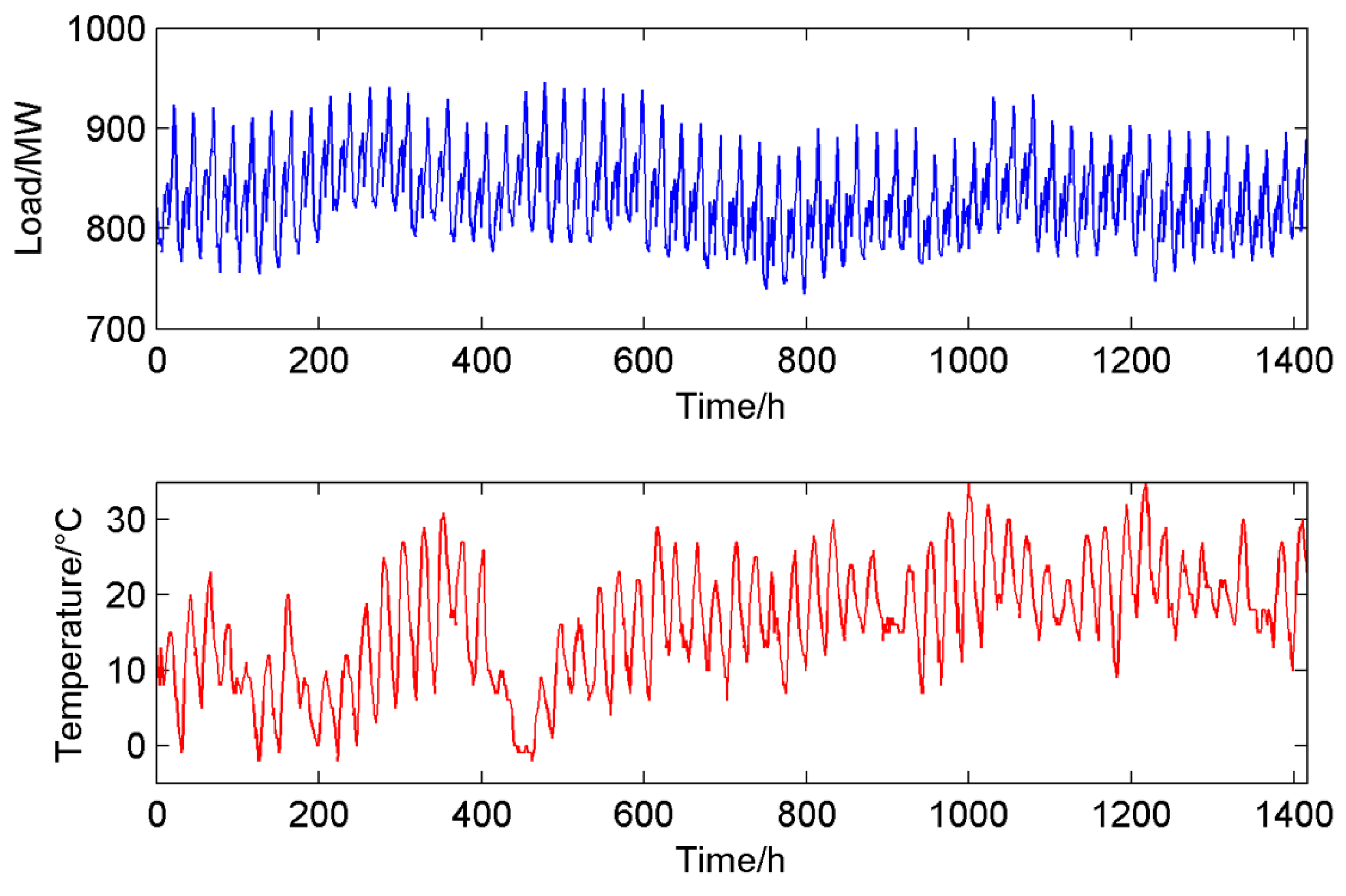
3.1. Data Preprocessing

This paper establishes a prediction model of short-term load forecasting and analyzes the prediction results of the examples. The 24-h short-term load forecasting has been made on the power system of Yangquan city in China from 1 April to 30 May 2013 (the load data of 23 May are missing). Figure 4 shows the power load of 1416 samples, ranging from around 730 MW to 950 MW. From Figure 4, no apparent regularity of power load can be obtained. In this paper, we select 708 load data from 1 to 30 April as the training set, 660 load data from 30 April to 28 May as the validation set and 72 load data from 29 to 31 May as the testing set.

The original load data are decomposed to eliminate the current precipitation value for further modeling by using WT. The original short-term load data S and their approximation A1, as well as the detail component D1 decomposed by one-level DWT are shown in Figure 5.

From Figure 5, it can be clearly seen that A1, which presents the major fluctuation of the original short-term load data, shows high similarity to S; meanwhile, the other minor irregularity neglected by A1 appears in D1. Therefore, A1 is taken as the input data to model for efficiency.

3.2. Selection of Input

Human activities are always disturbed by many external factors, and then, the power load is affected. Therefore, some effective features are considered as input features. In this paper, the input features are discussed as follows. (1) The temperature: Temperature is one of these effective features. In previous studies [37,38], temperature was considered as an essential input feature and the forecasting results were accurate enough. The curves of temperature and load data are shown in Figure 6. Therefore, the temperature is taken into consideration. (2) Weather conditions: The weather conditions are divided into four types: sunny, cloudy, overcast and rainy. For different weather conditions, we set different weights: {sunny, cloudy, overcast, rainy} = {0.8, 0.6, 0.4, 0.2}. (3) Day type: For different day types, the electric power consumption is different. Figure 7 shows the load data from 28 April to 4 May 2013. From Figure 7, we can see that different day types have different curve features. Therefore, we assign values to the day type in

Table 1. The values of the day type.

Day Type	Monday	Tuesday	Wednesday	Thursday	Friday	Saturday	Sunday
Weights	1	2	3	4	5	6	7

.

3.3. Model Performance Evaluation

The work in [39] discusses and compares the measures of the accuracy of univariate time series forecasts. According to this reference, the relative error (RE), the mean absolute percentage error (MAPE), the root mean square error (RMSE) and absolute error (AE) are proposed to measure the forecast accuracy. The equations are as follows:

$$RE(i)=\frac{{\widehat{y}}_i-y_i}{y_i}\times 100\%$$

(15)

$$MAPE=\frac{1}{n}{\displaystyle \sum _{i=1}^n\left|\frac{{\widehat{y}}_i-y_i}{y_i}\right|}$$

(16)

$$MSE=\frac{1}{n}{\displaystyle \sum _{i=1}^n{({\widehat{y}}_i-y_i)}^2}$$

(17)

$$AE=\left|\frac{{\widehat{y}}_i-y_i}{y_i}\times 100\%\right|$$

(18)

where $y_i$ represents the actual value at period $i$; ${\widehat{y}}_i$ is the forecasting value at period $i$; and $n$ is the number of forecasting period.

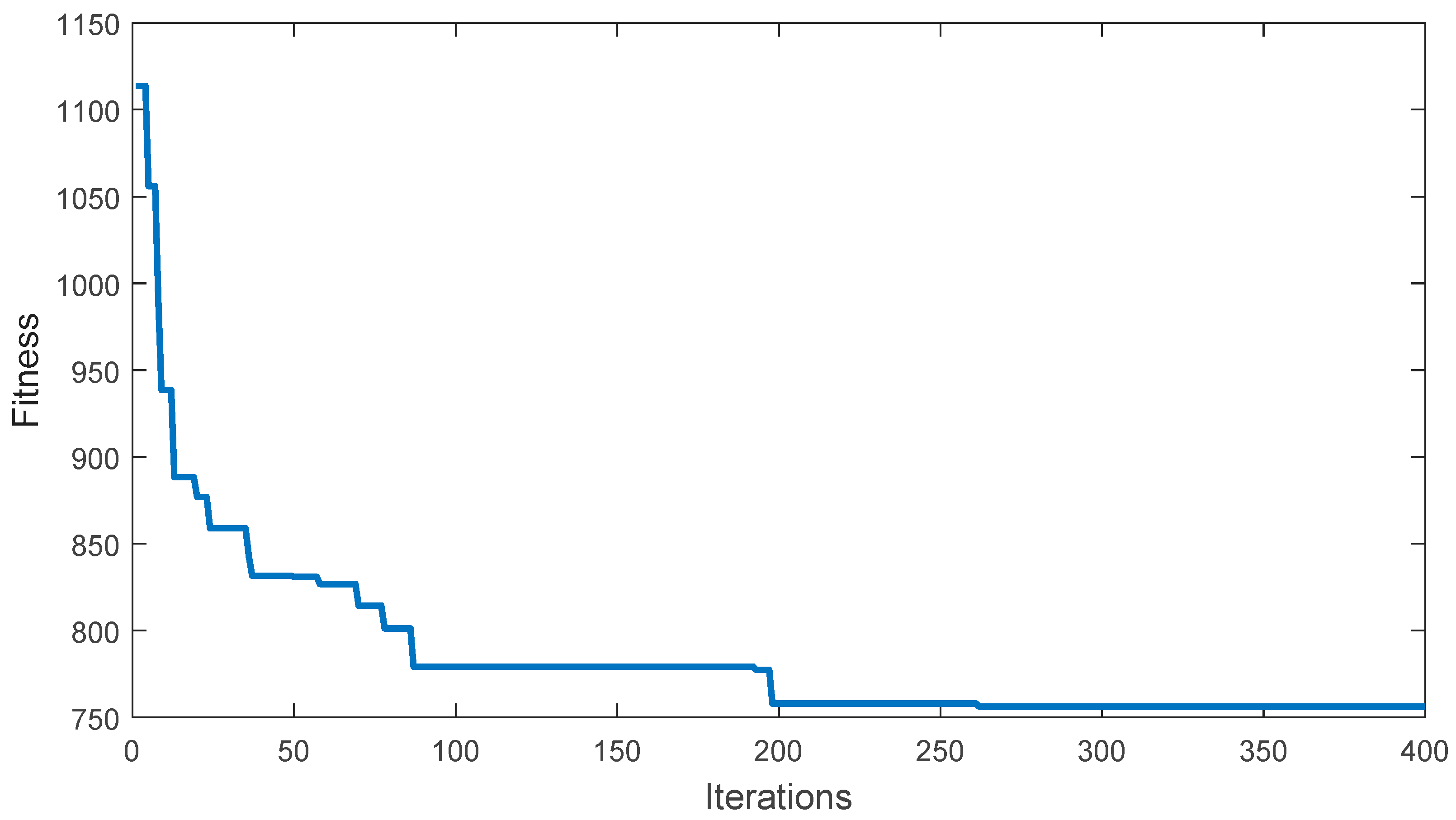
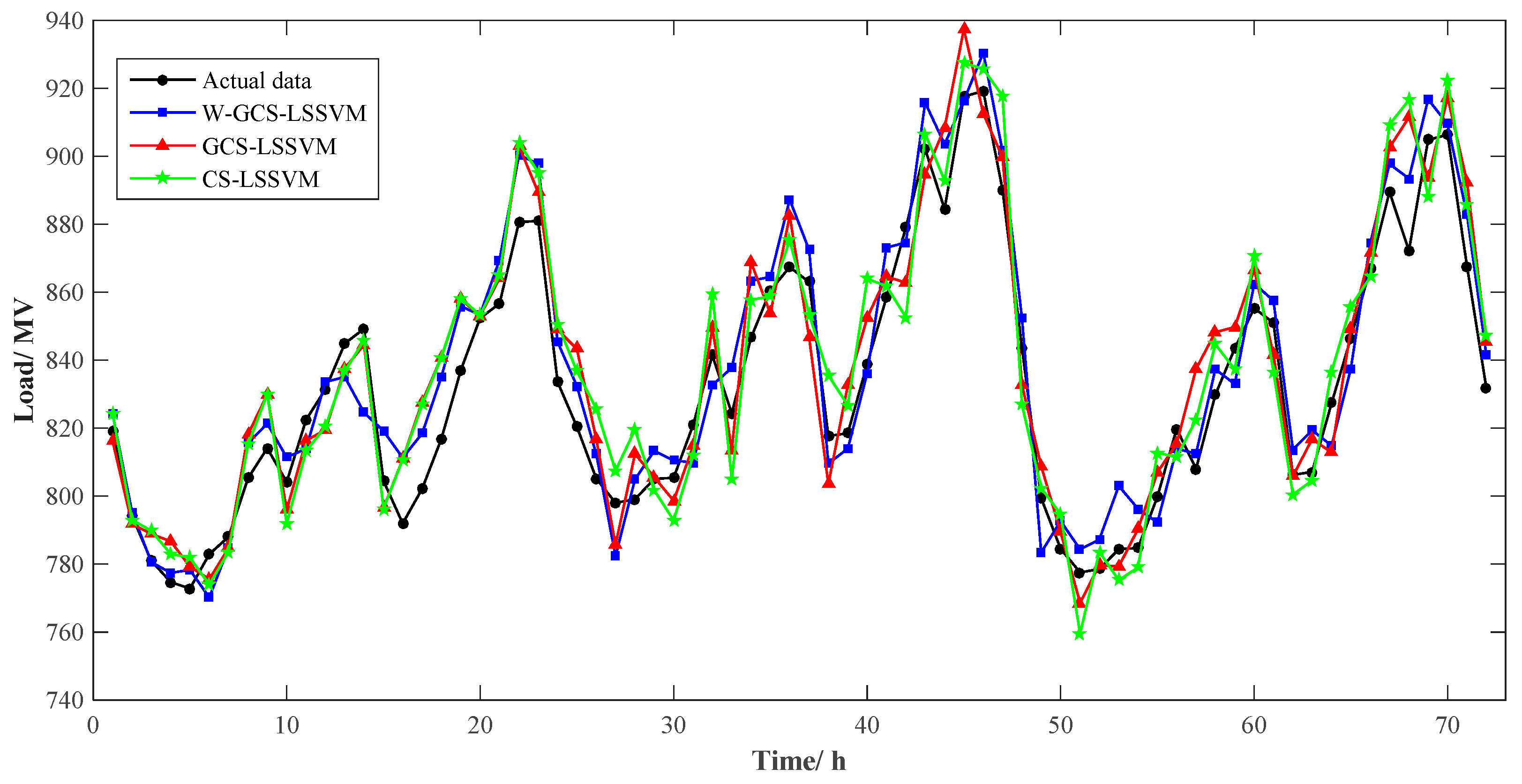
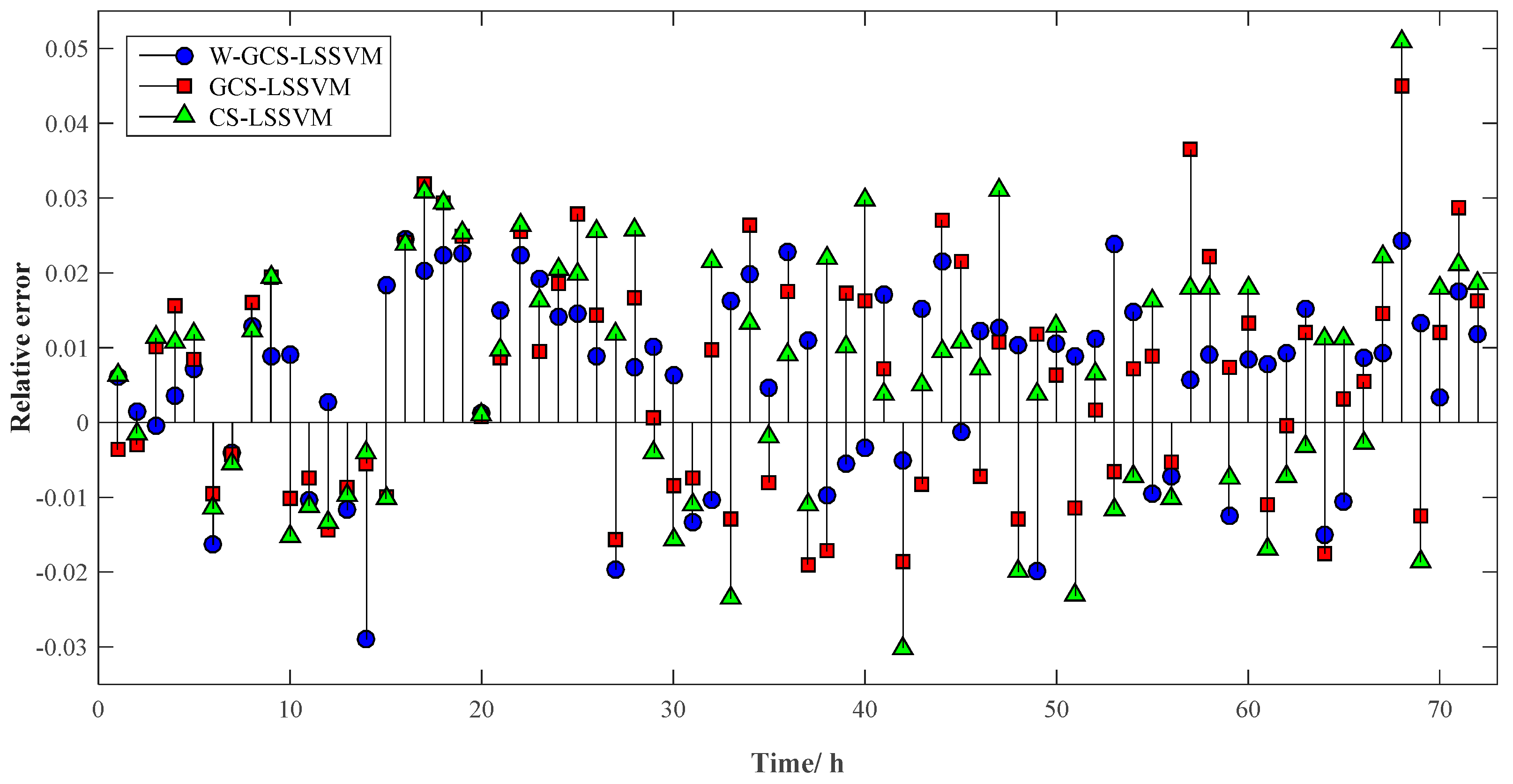
3.4. Analysis of Forecasting Results

At first, the GCS is used to optimize the kernel parameter ${\sigma }^2$ and penalty parameter $\gamma$ in LSSVM. The parameter settings of GCS is given in Section 2.4. Figure 8 shows the iterations process of GCS. From the figure we can see that GCS achieves convergence at 263 times. The optimal values of ${\sigma }^2$ and $\gamma$ are respectively 6.41 and 16.24.

The short-term electric load forecasting results of three days of the W-GCS-LSSVM, GCS-LSSVM, CS-LSSVM, W-LSSVM (${\sigma }^2=5$ and $\gamma =10$) and LSSVM (${\sigma }^2=5$ and $\gamma =10$) model are respectively shown in

Table 2. Actual load and forecasting results in Day 1 (Unit: MV).

Time/h	Actual Data	W-GCS-LSSVM	GCS-LSSVM	CS-LSSVM	W-LSSVM	LSSVM
D1 0:00	819.22	824.19	816.24	824.33	818.62	808.19
D1 1:00	794.17	795.39	791.85	793.01	794.81	792.45
D1 2:00	781	780.58	788.85	789.83	779.74	798.44
D1 3:00	774.72	777.43	786.75	782.96	785.82	778.57
D1 4:00	772.77	778.34	779.29	781.87	782.15	788.59
D1 5:00	782.96	770.16	775.57	773.96	771.73	757.91
D1 6:00	788.06	784.95	784.70	783.63	785.81	784.52
D1 7:00	805.28	815.59	818.14	815.14	813.85	831.05
D1 8:00	814.13	821.34	829.90	830.01	827.35	847.93
D1 9:00	804.14	811.42	795.91	791.91	817.41	809.03
D1 10:00	822.51	813.97	816.38	813.35	816.82	811.04
D1 11:00	831.4	833.61	819.48	820.36	833.63	814.20
D1 12:00	844.94	835.04	837.60	836.71	834.76	830.21
D1 13:00	849.24	824.61	844.59	845.87	820.82	866.12
D1 14:00	804.53	819.21	796.47	796.34	818.67	776.05
D1 15:00	791.98	811.29	810.95	810.87	811.38	810.86
D1 16:00	802.18	818.43	827.71	826.94	818.47	838.65
D1 17:00	816.86	835.09	840.89	840.88	845.26	843.89
D1 18:00	837.08	855.90	857.95	858.30	855.93	857.99
D1 19:00	852.35	853.37	853.06	853.28	853.40	869.15
D1 20:00	856.64	869.55	864.12	865.014	867.90	836.73
D1 21:00	880.66	900.40	903.09	903.91	899.78	902.18
D1 22:00	881	897.83	889.43	895.33	893.81	898.87
D1 23:00	833.55	845.33	848.99	850.65	845.25	865.29

,

Table 3. Actual load and forecasting results in Day 2 (Unit: MV).

Time/h	Actual Data	W-GCS-LSSVM	GCS-LSSVM	CS-LSSVM	W-LSSVM	LSSVM
D2 0:00	820.46	832.43	843.35	836.78	847.36	838.42
D2 1:00	805.16	812.32	816.74	825.76	814.57	818.54
D2 2:00	798.03	782.32	785.59	807.47	793.76	780.42
D2 3:00	799.06	804.94	812.42	819.58	815.87	773.23
D2 4:00	805.05	813.26	805.56	801.75	808.95	815.53
D2 5:00	805.42	810.52	798.67	792.84	822.46	815.34
D2 6:00	820.92	809.91	814.75	811.86	812.87	829.43
D2 7:00	841.42	832.62	849.53	859.54	821.74	832.58
D2 8:00	824.37	837.73	813.65	804.93	812.56	845.76
D2 9:00	846.60	863.42	868.87	857.75	842.43	832.43
D2 10:00	860.55	864.53	853.67	858.82	868.52	872.54
D2 11:00	867.44	887.29	882.56	875.26	893.65	851.76
D2 12:00	863.01	872.42	846.64	853.57	865.78	867.34
D2 13:00	817.65	809.64	803.56	835.53	826.68	825.86
D2 14:00	818.51	813.93	832.67	826.82	822.56	802.65
D2 15:00	839.02	836.22	852.57	863.98	824.75	823.75
D2 16:00	858.49	873.12	864.67	861.79	882.79	864.25
D2 17:00	879.16	874.64	862.76	852.65	877.53	885.29
D2 18:00	902.11	915.82	894.73	906.64	907.75	924.63
D2 19:00	884.54	903.54	908.47	892.88	908.64	899.43
D2 20:00	917.62	916.37	937.43	927.45	927.65	934.54
D2 21:00	919.17	930.48	912.57	925.75	937.73	902.43
D2 22:00	890.22	901.54	899.73	917.84	906.43	914.35
D2 23:00	843.72	852.45	832.76	826.87	862.58	872.43

and

Table 4. Actual load and forecasting results in Day 3 (Unit: MV).

Time/h	Actual Data	W-GCS-LSSVM	GCS-LSSVM	CS-LSSVM	W-LSSVM	LSSVM
D3 0:00	799.38	783.43	808.87	802.43	787.86	813.50
D3 1:00	784.48	792.66	789.43	794.62	801.54	806.64
D3 2:00	777.53	784.34	768.59	759.52	781.48	785.74
D3 3:00	778.53	787.23	779.76	783.59	793.78	782.74
D3 4:00	784.36	802.98	779.25	775.24	794.65	805.99
D3 5:00	784.72	796.32	790.31	778.98	804.92	790.22
D3 6:00	799.83	792.23	806.98	812.76	787.77	811.39
D3 7:00	819.81	813.87	815.42	811.46	826.41	819.27
D3 8:00	808.02	812.59	837.49	822.54	802.83	812.74
D3 9:00	829.81	837.31	848.26	844.72	823.75	836.71
D3 10:00	843.49	832.98	849.72	837.28	845.48	850.32
D3 11:00	855.36	862.48	866.74	870.62	867.74	877.88
D3 12:00	850.99	857.55	841.53	836.66	852.65	880.61
D3 13:00	806.26	813.69	805.87	800.43	825.98	830.73
D3 14:00	807.11	819.43	816.76	804.58	814.65	825.97
D3 15:00	827.34	814.87	812.83	836.65	810.54	853.78
D3 16:00	846.53	837.49	849.23	855.92	823.65	874.95
D3 17:00	866.92	874.43	871.59	864.46	863.42	894.91
D3 18:00	889.56	897.78	902.57	909.34	902.67	908.75
D3 19:00	872.23	893.45	911.48	916.56	897.85	877.78
D3 20:00	904.85	916.77	893.56	887.94	924.43	898.62
D3 21:00	906.38	909.49	917.34	922.54	916.49	926.14
D3 22:00	867.61	882.73	892.52	885.91	877.61	853.82
D3 23:00	831.98	841.76	845.46	847.43	835.64	856.50

. In order to explain the results more clearly, the proposed model and comparison models are divided into two groups: the first group includes W-GCS-LSSVM, GCS-LSSVM and CS-LSSVM, and the second group consists of W-GCS-LSSVM, W-LSSVM and LSSVM, which are respectively shown in Figure 9 and Figure 10. Moreover, Figure 11 and Figure 12 show the comparisons of relative errors between the proposed model and the others. The RE ranges [−3%, 3%] and [−1%, 1%] are popularly regarded as a standard to evaluate the performance of a prediction model [40]. Based on these tables and figures, we can obtain that: (1) the REs of the short-term load forecasting model of W-GCS-LSSVM are all in the range of [−3%, 3%]; the maximum RE is 2.4380% at 15:00 (Day 1), and the minimum RE is −2.901% at 13:00 (Day 1); there exists thirty points that are in the scope of [−1%, 1%]; (2) the GCS-LSSVM has three predicted points that exceed the RE range [−3%, 3%], which are 4.5000% at 19:00 (Day 3), 3.6472% at 8:00 (Day 3) and 3.1826% at 16:00 (Day 1), and there are twenty-nine predicted points in the range of [−1%, 1%]; (3) the CS-LSSVM has four predicted points that exceed the RE range [−3%, 3%], which are 5.0824% at 19:00 (Day 3), 3.1026% at 22:00 (Day 2), 3.0863% at 16:00 (Day 1) and −3.0154% at 17:00 (Day 2), and there are twenty-one predicted points in the range of [−1%, 1%]; (4) the W-LSSVM has four predicted points that exceed the RE range [−3%, 3%], which are respectively 3.4763% at 17:00 (Day 1), 3.2786% at 0:00 (Day 2), 3.0215% at 11:00 (Day 2) and −3.3465% at 13:00 (Day 1), and there are seventeen predicted points in the range of [−1%, 1%]; (5) the single LSSVM has fourteen predicted points that exceed the RE range [−3%, 3%], which are respectively 4.1518% at 8:00 (Day 1), 3.8082% at 23:00 (Day 1), 3.4807% at 12:00 (Day 3), 3.4028% at 23:00 (Day 2), 3.3572% at 16:00 (Day 3), 3.3091% at 17:00 (Day 1), 3.2287% at 17:00 (Day 3), 3.1997% at 7:00 (Day 1), 3.1958% at 15:00 (Day 3), 3.0350% at 13:00 (Day 3), −3.1991% at 5:00 (Day 1), −3.2325% at 3:00 (Day 2) and −3.5397% at 14:00 (Day 1), and there are fifteen predicted points in the range of [−1%, 1%]. From the global view of RE, the forecasting accuracy of W-GCS-LSSVM is better than the other models, since it has the most predicted points in the ranges [−1%, 1%] and [−3%, 3%]. Moreover, from Figure 9, the results of GCS-LSSVM are better than those of CS-LSSVM, which can verify that the Gauss disturbance strategy applied in CS increases the vitality of the change of the nest position, thus improving the convergence speed and search ability effectively. From Figure 10, the effects of W-LSSVM are better than single LSSVM, which can illustrate that WT effectively filters the original data. However, the comparison models also predict more accurately than the proposed model at some points, for example the RE of W-GCS-LSSVM is 2.901% at 13:00 (Day 1), which is higher than that of GCS-LSSVM, CS-LSSVM and LSSVM.

The MAPE and MSE of WT-GCS-LSSVM, GCS-LSSVM, CS-LSSVM, W-LSSVM and LSSVM are listed in

Table 5. Model performance evaluations.

Model	W-GCS-LSSVM	GCS-LSSVM	CS-LSSVM	W-LSSVM	LSSVM
MAPE	1.2083%	1.3682%	1.4790%	1.4213%	1.9557%
MSE	131.6950	185.6538	210.7736	196.6906	336.5224

. From Table 5, we can conclude that the MAPE of the proposed model is 1.2083%, which is smaller than the MAPE of GCS-LSSVM, CS-LSSVM, W-LSSVM and LSSVM (which are 1.3682%, 1.4790%, 1.4213% and 1.9557%). In addition, the MSE of the proposed model is 131.6950, which is smaller than the MSE of the comparison models (which are 185.6538, 210.7736, 196.6906 and 336.5224). As a result, the MAPE and MSE of the W-GCS-LSSVM are both smaller than those of the W-LSSVM, so we can conclude that the parameter optimization to LSSVM is essential in the forecasting model. Besides, the MAPE and MSE of the WT-GCS-LSSVM are both smaller than GCS-LSSVM, indicating the pre-processing of load data is useful for a better performance and higher forecasting accuracy. At the same time, the MAPE and MSE of the GCS-LSSVM and CS-LSSVM are both smaller than those of LSSVM, and this presents that the optimization results of the GCS and CS are efficient.

In addition, the AE of the load forecasting value divided into four parts that is calculated from Equation (18) is shown in Figure 13. The numbers on the x-axis represent the models appeared above: 1 represents the W-GCS-LSSVM model, 2 represents the GCS-LSSVM model, 3 represents the CS-LSSVM model, 4 represents the W-LSSVM model and 5 represents the single LSSVM model. From Figure 13, we can discover that the AE values of W-GCS-LSSVM are almost lower than those of the other models. The numbers of points that are less than 1%, 3% and more than 3% and the corresponding percentage of them in the predicted points are accounted, respectively. The statistical results are shown in

Table 6. Accuracy estimation of the prediction point for the test set.

Prediction Model	<1%		>1% and <3%		≥3%
	Number	Percentage	Number	Percentage	Number	Percentage
W-GCS-LSSVM	30	41.67%	42	58.33%	0	0%
GCS-LSSVM	29	40.28%	40	55.56%	3	4.17%
CS-LSSVM	21	29.17%	47	65.28%	4	5.56%
W-LSSVM	25	34.72%	43	59.72%	4	5.56%
LSSVM	15	20.83%	43	59.72%	14	19.44%

. It can be seen that there are 30 predicted points whose the AE of the W-GCS-LSSVM model is less than 1%, which accounts for 41.67% of the total amount; and 42 predicted points less than 3%, accounting for 58.33% of the total amount. Besides, there are no number predicted points whose AE is more than 3%, accounting for 0% of the total amount. It can be indicated that the prediction performance of the proposed model is superior, and its accuracy is higher. Therefore, the W-GCS-LSSVM model is suitable for short-term load forecasting.

4. Conclusions

To strengthen the stability and economy of the grid and avoid waste in grid scheduling, it is essential to improve the forecasting accuracy. Because the short-term power load is always interfered with by various external factors with characteristics like high volatility and instability, the high accuracy of load forecasting should be taken into consideration. Based on the features of load data and the randomness of the LSSVM parameter setting, we propose the model based on wavelet transform and least squares support vector machine optimized by improved cuckoo search. To validate the proposed model, four other comparison models (GCS-LSSVM, CS-LSSVM, W-LSSVM and LSSVM) are employed to compare the forecasting results. Example computation results show that the relative errors of the W-GCS-LSSVM model are all in the range of [−3%, 3%], and the MAPE and MSE are both smaller than the others. In addition, the advantage of CS is that it does not have many parameters for tuning, so it can be applied widely in parameter optimization. However, seasonality and long-term trend of the proposed model are not tested and verified in this paper, which may become the limitation of this method, and authors will study it in the future. Above all, the hybrid model can be effectively used in the short-term load forecasting on the power system.

References

1. Bozic, M.; Stojanovic, M.; Stajic, Z.; Tasić, D. A new two-stage approach to short term electrical load forecasting. Energies 2013, 6, 2130–2148. [Google Scholar] [CrossRef]
2. Liang, R.H.; Chen, Y.K.; Chen, Y.T. Volt/Var control in a distribution system by a fuzzy optimization approach. Int. J. Electr. Power Energy Syst. 2011, 33, 278–287. [Google Scholar] [CrossRef]
3. Niknam, T.; Zare, M.; Aghaei, J. Scenario-based multiobjective Volt/Var control in distribution networks including renewable energy sources. IEEE Trans. Power Deliv. 2012, 27, 2004–2019. [Google Scholar] [CrossRef]
4. Lee, C.M.; Ko, C.N. Short-term load forecasting using lifting scheme and ARIMA models. Expert Syst. Appl. 2011, 38, 5902–5911. [Google Scholar] [CrossRef]
5. Pappas, S.S.; Ekonomou, L.; Karamousantas, D.C.; Chatzarakis, G.E.; Katsikas, S.K.; Liatsis, P. Electricity demand loads modeling using Auto Regressive Moving Average (ARMA) models. Energy 2008, 33, 1353–1360. [Google Scholar] [CrossRef]
6. Pappas, S.S.; Ekonomou, L.; Karampelas, P.; Karamousantasd, D.C.; Katsikase, S.K.; Chatzarakis, G.E.; Skafidas, P.D. Electricity demand load forecasting of the Hellenic power system using an ARMA model. Electr. Power Syst. Res. 2010, 80, 256–264. [Google Scholar] [CrossRef]
7. Kandil, N.; Wamkeue, R.; Saad, M.; Georges, S. An efficient approach for short term load forecasting using artificial neural networks. Int. J. Electr. Power Energy Syst. 2006, 28, 525–530. [Google Scholar] [CrossRef]
8. Yu, F.; Xu, X. A short-term load forecasting model of natural gas based on optimized genetic algorithm and improved BP neural network. Appl. Energy 2014, 134, 102–113. [Google Scholar] [CrossRef]
9. Chaturvedi, D.K.; Sinha, A.P.; Malik, O.P. Short term load forecast using fuzzy logic and wavelet transform integrated generalized neural network. Int. J. Electr. Power Energy Syst. 2015, 67, 230–237. [Google Scholar] [CrossRef]
10. Hernandez, L.; Baladrón, C.; Aguiar, J.M.; Carro, B.; Sanchez-Esguevillas, A.J.; Lloret, J. Short-Term Load Forecasting for Microgrids Based on Artificial Neural Networks. Energies 2013, 6, 1385–1408. [Google Scholar] [CrossRef]
11. Amjady, N.; Keynia, F. A new neural network approach to short term load forecasting of electrical power systems. Energies 2011, 4, 488–503. [Google Scholar] [CrossRef]
12. Pan, D.; Xie, K.; Guo, T.; Huang, X. Short-term load forecasting for electric power systems using the PSO-SVR and FCM clustering techniques. Energies 2011, 4, 173–184. [Google Scholar]
13. Kavousi-Fard, A.; Samet, H.; Marzbani, F. A new hybrid Modified Firefly Algorithm and Support Vector Regression model for accurate Short Term Load Forecasting. Expert Syst. Appl. 2014, 41, 6047–6056. [Google Scholar] [CrossRef]
14. Vapnik, V. The Nature of Statistical Learning Theory; Springer Science & Business Media: Berlin, Germany, 2000. [Google Scholar]
15. Sun, W.; Liang, Y. Least-Squares Support Vector Machine Based on Improved Imperialist Competitive Algorithm in a Short-Term Load Forecasting Model. J. Energy Eng. 2014, 141, 04014037. [Google Scholar] [CrossRef]
16. Mesbah, M.; Soroush, E.; Azari, V.; Lee, M.; Bahadori, A.; Habibnia, S. Vapor liquid equilibrium prediction of carbon dioxide and hydrocarbon systems using LSSVM algorithm. J. Supercrit. Fluids 2015, 97, 256–267. [Google Scholar] [CrossRef]
17. Liu, H.; Yao, X.; Zhang, R.; Liu, M.; Hu, Z.; Fan, B. Accurate quantitative structure-property relationship model to predict the solubility of C60 in various solvents based on a novel approach using a least-squares support vector machine. J. Phys. Chem. B 2005, 109, 20565–20571. [Google Scholar] [CrossRef] [PubMed]
18. Sun, W.; Liang, Y. Research of least squares support vector regression based on differential evolution algorithm in short-term load forecasting model. J. Renew. Sustain. Energy 2014, 6, 053137. [Google Scholar] [CrossRef]
19. Sun, W.; Liu, M.H.; Liang, Y. Wind speed forecasting based on FEEMD and LSSVM optimized by the bat algorithm. Energies 2015, 8, 6585–6607. [Google Scholar] [CrossRef]
20. Sun, W.; Liang, Y. Comprehensive evaluation of cleaner production in thermal power plants using particle swarm optimization based least squares support vector machines. J. Inf. Comput. Sci. 2015, 12, 1993–2000. [Google Scholar] [CrossRef]
21. Sun, W.; Liang, Y.; Xu, Y.F. Application of carbon emissions prediction using least squares support vector machine based on grid search. WSEAS Trans. Syst. Control 2015, 10, 95–104. [Google Scholar]
22. Gorjaei, R.G.; Songolzadeh, R.; Torkaman, M.; Safari, M.; Zargar, G. A novel PSO-LSSVM model for predicting liquid rate of two phase flow through wellhead chokes. J. Nat. Gas Sci. Eng. 2015, 24, 228–237. [Google Scholar] [CrossRef]
23. Liu, D.; Niu, D.; Wang, H.; Fan, L. Short-term wind speed forecasting using wavelet transform and support vector machines optimized by genetic algorithm. Renew. Energy 2014, 62, 592–597. [Google Scholar] [CrossRef]
24. Yang, X.S.; Deb, S. Cuckoo Search via Levy Flights. In Proceedings of the World Congress on IEEE 2010, Barcelona, Spain, 18–23 July 2010.
25. Valian, E.; Tavakoli, S.; Mohanna, S.; Haghi, A. Improved cuckoo search for reliability optimization problems. Comput. Ind. Eng. 2013, 64, 459–468. [Google Scholar] [CrossRef]
26. Wong, P.K.; Wong, K.I.; Chi, M.V.; Cheung, C.S. Modelling and optimization of biodiesel engine performance using kernel-based extreme learning machine and cuckoo search. Renew. Energy 2015, 74, 640–647. [Google Scholar] [CrossRef]
27. Abdelaziz, A.Y.; Ali, E.S. Cuckoo Search algorithm based load frequency controller design for nonlinear interconnected power system. Int. J. Electr. Power Energy Syst. 2015, 73, 632–643. [Google Scholar] [CrossRef]
28. Wang, J.; Jiang, H.; Wu, Y.; Dong, Y. Forecasting solar radiation using an optimized hybrid model by Cuckoo Search algorithm. Energy 2015, 81, 627–644. [Google Scholar] [CrossRef]
29. Deihimi, A.; Orang, O.; Showkati, H. Short-term electric load and temperature forecasting using wavelet echo state networks with neural reconstruction. Energy 2013, 57, 382–401. [Google Scholar] [CrossRef]
30. Abdoos, A.; Hemmati, M.; Abdoos, A.A. Short term load forecasting using a hybrid intelligent method. Knowl.-Based Syst. 2015, 76, 139–147. [Google Scholar] [CrossRef]
31. Chen, J.; Li, Z.; Pan, J.; Chen, G.; Zi, Y.; Yuan, J.; Chen, B.; He, Z. Wavelet transform based on inner product in fault diagnosis of rotating machinery: A review. Mech. Syst. Signal Process. 2016, 70, 1–35. [Google Scholar] [CrossRef]
32. Zhang, Y.; Li, H.; Wang, Z.; Li, J. A preliminary study on time series forecast of fair-weather atmospheric electric field with WT-LSSVM method. J. Electrost. 2015, 75, 85–89. [Google Scholar] [CrossRef]
33. Shayeghi, H.; Ghasemi, A. Day-ahead electricity prices forecasting by a modified CGSA technique and hybrid WT in LSSVM based scheme. Energy Convers. Manag. 2013, 74, 482–491. [Google Scholar] [CrossRef]
34. Suykens, J.A.K.; Vandewalle, J. Least squares support vector machine classifiers. Neural Process. Lett. 1999, 9, 293–300. [Google Scholar] [CrossRef]
35. Sun, W.; Liang, Y. Least-squares support vector machine based on improved imperialist competitive algorithm in a short-term load forecasting model. J. Energy Eng. 2015, 141, 04014037. [Google Scholar] [CrossRef]
36. Yang, X.S.; Deb, S. Engineering optimisation by cuckoo search. Int. J. Math. Model. Numer. Optim. 2010, 1, 330–343. [Google Scholar] [CrossRef]
37. Hooshmand, R.A.; Amooshahi, H.; Parastegari, M. A hybrid intelligent algorithm based short-term load forecasting approach. Int. J. Electr. Power Energy Syst. 2013, 45, 313–324. [Google Scholar] [CrossRef]
38. Bahrami, S.; Hooshmand, R.A.; Parastegari, M. Short term electric load forecasting by wavelet transform and grey model improved by PSO (particle swarm optimization) algorithm. Energy 2014, 72, 434–442. [Google Scholar] [CrossRef]
39. Hyndman, R.J.; Koehler, A.B. Another look at measures of forecast accuracy. Int. J. Forecast. 2006, 22, 679–688. [Google Scholar] [CrossRef]
40. Niu, D.; Wang, Y.; Wu, D.D. Power load forecasting using support vector machine and ant colony optimization. Expert Syst. Appl. 2010, 37, 2531–2539. [Google Scholar] [CrossRef]
Figure 1. Wavelet decomposition.
Energies 09 00827 g001
Figure 2. The pseudo-code of the cuckoo search (CS).
Energies 09 00827 g002
Figure 3. Flowchart of the W-CS algorithm based on Gauss disturbance (GCS)-least squares support vector machine (LSSVM) modeling.
Energies 09 00827 g003
Figure 4. Load curve for each hour.
Energies 09 00827 g004
Figure 5. Original load signal and its approximation component and detail component decomposed by DWT.
Energies 09 00827 g005
Figure 6. The curves of the load data and temperature.
Energies 09 00827 g006
Figure 7. Weekly load curve.
Energies 09 00827 g007
Figure 8. The iterations process of GCS.
Energies 09 00827 g008
Figure 9. Actual load and forecasting results of W-GCS-LSSVM, GCS-LSSVM and CS-LSSVM.
Energies 09 00827 g009
Figure 10. Actual load and forecasting results of W-GCS-LSSVM, W-LSSVM and LSSVM.
Energies 09 00827 g010
Figure 11. Relative Errors of W-GCS-LSSVM, GCS-LSSVM and CS-LSSVM.
Energies 09 00827 g011
Figure 12. Relative Errors of W-GCS-LSSVM, W-LSSVM and LSSVM.
Energies 09 00827 g012
Figure 13. Absolute error distribution curve for different models, (a) the AE value from 1 to 18 sample point; (b) the AE value from 19 to 36 sample point; (c) the AE value from 37 to 54 sample point; (d) the AE value from 55 to 72 sample point.
Energies 09 00827 g013