Risk-Limiting Scheduling of Optimal Non-Renewable Power Generation for Systems with Uncertain Power Generation and Load Demand

Abstract

This study tackles a risk-limiting scheduling problem of non-renewable power generation for large power systems, and addresses potential violations of the security constraints owing to the volatility of renewable power generation and the uncertainty of load demand. To cope with the computational challenge that arises from the probabilistic constraints in the considered problem, a computationally efficient solution algorithm that involves a bisection method, an off-line constructed artificial neural network (ANN) and an on-line point estimation method is proposed and tested on the IEEE 118-bus system. The results of tests and comparisons reveal that the proposed solution algorithm is applicable to large power systems in real time, and the solution obtained herein is much better than the conventional optimal power flow (OPF) solution in obtaining a much higher probability of satisfying the security constraints.

1. Introduction

There is a growing interest in utilizing renewable energy such as wind and solar as the power generation sources to overcome the global climate change induced by carbon emission [1,2,3,4]. Additionally, the economic incentives based demand response has prevailed recently to improve the efficiency of electricity utilization and reduce carbon emission [5]. However, to integrate the distributed renewable energy sources and increase the participation of demand response, it is necessary to transform the traditional electricity grid into a smart grid [6]. The smart grid itself is simply the application of modern communication infrastructure to various segments of the electricity grid. However, the intermittency of the electricity supplied by renewable energy sources and the uncertain load demand caused by demand response in a modern power system require some traditional power system operations to consider these uncertainties [7,8]. For example, Dvorkin et al. [9] used a hybrid stochastic/interval approach to tackle the transmission-constrained unit commitment problem with uncertainties of wind power generation and load demand. Wu et al. [10] proposed a day-ahead stochastic scheduling model to cope with the hourly forecast errors of system loads and variable renewable sources. Ahmadi-Khatir et al. [11] proposed a decentralized method to optimally schedule generating units for systems under wind power uncertainties. Kusiak et al. discuss wind turbine capacity [12]. In this paper, the schedule of non-renewable power generation in a large power system with uncertain power generation and load demand is under consideration.

The challenge posed by uncertain power generation and load demand in scheduling the non-renewable power generation is to maintain the power balance at all times and satisfy the security constraints on the security terms of interest, which are the bus voltage magnitude and the transmission line real power flow. In general, the scheduled value of optimal non-renewable power generation is the solution of optimal power flow (OPF), in which the renewable power generation and load demand are set to their predicted values, which differ from the actual values and cause a power mismatch in practice. Accordingly, the system operator should re-dispatch the scheduled optimal non-renewable power generation to maintain the power balance. This re-dispatch may cause the security constraints violated. Therefore, the purpose of this paper is to find a risk-limiting schedule of optimal non-renewable power generation to reduce the probability of violating security constraints after the re-dispatch in the presence of uncertain power generation and load demand. In past decades, numerous mathematical programming methods for solving deterministic OPF problems of the traditional electricity grid were proposed. For example, the successive linear programming method [13], the successive quadratic programming method [14], the Lagrange Newton method [15], the primal-dual interior point method [16], the dual-type method [17], the multi-objective programming method [18], the hybrid algorithm [19], the modified shuffle frog leaping (SFL) algorithm [20], the population based algorithm [21], etc. However, the aforementioned methods cannot be used to solve the problem considered in this paper.

Setting restrictive bounds for the security constraints in the OPF problem formulation can reduce the risk of violating the security constraints in practice; however, more restrictive bounds result in a larger scheduled optimal non-renewable power generation cost. Therefore, to minimize the scheduled optimal non-renewable power generation cost, the problem formulation of the proposed risk-limiting schedule of optimal non-renewable power-generation (RSONP) is to determine the least restrictive bounds that yield the required probability of satisfying the security constraints after the re-dispatch. Few articles have discussed this issue. Although Varaiya et al. [22] proposed a dispatch method with limiting risk, they ignored security constraints and considered only the need for power generation to satisfy load demand. Attaching a probability to the satisfaction of security constraints, Zhang and Li [23] developed a chance constrained programming (CCP) method for solving OPF with load uncertainty. Lin and Lin [24] proposed a risk-limiting OPF (RLOPF) method to solve the RLOPF problem for systems with a high penetration of wind power; however, they did not take into account the uncertainty of load demand. Therefore, the RSONP problem with uncertain power generation and load demand remains unsolved. Furthermore, both the CCP method and the RLOPF method were experimentally tested using small systems [23,24]. Hence, the contribution of this paper is to propose a computationally efficient RSONP algorithm to solve the RSONP problem of a large power system.

This paper is organized as follows. Section 2 presents the method for solving the RSONP problem. Section 3 presents the test results and discussions. Section 4 presents the conclusions and further research.

2. Method

2.1. Statement and Computational Challenges of Risk-Limiting Schedule of Optimal Non-Renewable Power-Generation Problem

For simplicity of presentation, the only renewable energy source considered herein is wind. However, solar power can be easily included in the formulated RSONP problem and the proposed RSONP algorithm.

2.1.1. Conventional Optimal Power Flow Problem

The OPF problem has various formulations. In this paper, the following conventional optimal power flow (COPF) problem is considered [8].

$$\begin{array}{ccc}\text{subject to}:& & \begin{array}{l}\underset{u_{G_i},i\in G\backslash WG}{\text{min}}{\displaystyle \sum _{i\in G\backslash WG}{a}_i{P}_{G_i}^2+b_i}{P}_{G_i}+c_i\\ g(x,u_G,{\widehat{u}}_W,{\widehat{u}}_D)=0\\ {\underset{\_}{p}}_{ij}^o\le p_{ij}(x_i,x_j)\le {\overline{p}}_{ij}^o, \forall (i,j)\in L\\ {\underset{\_}{V}}_i^o\le V_i\le {\overline{V}}_i^o, i=1,\cdots ,N\\ {\underset{\_}{u}}_{G_i}\le u_{G_i}\le {\overline{u}}_{G_i}, \forall i\in G\backslash WG\end{array}\end{array}$$

(1)

where ${\underset{\_}{V}}_i^o\le V_i\le {\overline{V}}_i^o, i=1,\cdots ,N,$ and ${\underset{\_}{p}}_{ij}^o\le p_{ij}(x_i,x_j)\le {\overline{p}}_{ij}^o$, $\forall (i,j)\in L$ represent the set of security constraints with normal bounds; and ${\underset{\_}{u}}_{G_i}\le u_{G_i}\le {\overline{u}}_{G_i}$ represents the power generation constraint at bus $i$. Normally, ${\underset{\_}{V}}_i^o=0.95$, ${\overline{V}}_i^o=1.05$ and ${\underset{\_}{p}}_{ij}^o=-{\overline{p}}_{ij}^o$. For notational simplicity, the aforementioned security constraints are rewritten as ${\underset{\_}{h}}_j^o\le h_j(x)\le {\overline{h}}_j^o$, $j=1,\cdots ,m$, where $m=N+|L|$, and $|L|$ is the total number of transmission lines, so $m$ is the total number of security constraints. Notably, ${\underset{\_}{h}}_j^o=-{\overline{h}}_j^o$ for the transmission line real power flow, and the renewable power generation is assumed to have no cost.

2.1.2. Statement of Risk-Limiting Schedule of Optimal Non-Renewable Power-Generation Problem

As indicated in Section 1, the RSONP problem is to determine the least restrictive bounds for security constraints in the OPF problem formulation that yield the required probability η that the security constraints will be satisfied in practice as follows:

$$\underset{{\underset{\_}{\mathbf{h}}}^s,{\overline{\mathbf{h}}}^s}{\text{min}}{\displaystyle \sum _{j=1}^m[({\underset{\_}{h}}_j^s}-{\underset{\_}{h}}_j^o{)}^2+{({\overline{h}}_j^o-{\overline{h}}_j^s)}^2]$$

subject to:

$$\text{Prob}\{{\underset{\_}{h}}_j^o\le h_j({\tilde{x}}^s)\le {\overline{h}}_j^o|{\underset{\_}{\mathbf{h}}}^s,{\overline{\mathbf{h}}}^s\}\ge \mathsf{\eta }, j=1,\cdots ,m$$

(2)

where ${\tilde{x}}^s$ represents the random state-vector after re-dispatching (RSAR), which is resulted from the scheduling and re-dispatching stages that will be presented later. $\text{Prob}\{{\underset{\_}{h}}_j^o\le h_j({\tilde{x}}^s)\le {\overline{h}}_j^o|{\underset{\_}{\mathbf{h}}}^s,{\overline{\mathbf{h}}}^s\}$ represents the conditional probability of satisfying the $j$th security constraint after the re-dispatch for the given restrictive bounds $({\underset{\_}{\mathbf{h}}}^s,{\overline{\mathbf{h}}}^s)$, and the objective function is the distance between the restrictive bounds $({\underset{\_}{\mathbf{h}}}^s,{\overline{\mathbf{h}}}^s)$ and the normal bounds $({\underset{\_}{\mathbf{h}}}^o,{\overline{\mathbf{h}}}^o)$. Therefore, the RSONP problem is to find the $({\underset{\_}{\mathbf{h}}}^s,{\overline{\mathbf{h}}}^s)$ that is closest to $({\underset{\_}{\mathbf{h}}}^o,{\overline{\mathbf{h}}}^o)$ while satisfying the conditional probability constraints in Equation (2).

2.1.3. Monte Carlo Simulation Procedures for Evaluating Exact Conditional Probability of Satisfying Security Constraints

For the given $({\underset{\_}{\mathbf{h}}}^s,{\overline{\mathbf{h}}}^s)$, the procedures to evaluate the exact value of $\text{Prob}\{{\underset{\_}{h}}_j^o\le h_j({\tilde{x}}^s)\le {\overline{h}}_j^o|{\underset{\_}{\mathbf{h}}}^s,{\overline{\mathbf{h}}}^s\}$ are described below.

• Scheduling Stage

In the scheduling stage, both wind power generation and load demand are set to their predicted values in the OPF problem with restrictive bounds $({\underset{\_}{\mathbf{h}}}^s,{\overline{\mathbf{h}}}^s)$ (OPFPRB), which is expressed as Equation (3).

$$\begin{array}{ccc}\text{subject to}:& & \begin{array}{l}\underset{u_{G_i},i\in G\backslash WG}{\text{min}}{\displaystyle \sum _{i\in G\backslash WG}{a}_i{P}_{G_i}^2+b_i}{P}_{G_i}+c_i\\ g(x,u_G,{\widehat{u}}_W,{\widehat{u}}_D)=0\\ {\underset{\_}{h}}_j^s\le h_j(x)\le {\overline{h}}_j^s, j=1,\cdots ,m\\ {\underset{\_}{u}}_{G_i}\le u_{G_i}\le {\overline{u}}_{G_i}, \forall i\in G\backslash WG\end{array}\end{array}$$

(3)

The solution of OPFPRB is denoted by $u_{G_i}^{s*}$, $\forall i\in G\backslash WG$, and is called the scheduled optimal non-renewable power-generation (SONP) for the given restrictive bounds $({\underset{\_}{\mathbf{h}}}^s,{\overline{\mathbf{h}}}^s)$.

• Random Generation of Wind Speed and Load Demand

The wind speed $v_l$ is a random variable, so is the wind power generation ${\tilde{u}}_{W_l}(v_l)$. Although the actual load demand for all buses, ${\tilde{u}}_{D_i}, i=1,\cdots ,N,$ are also random variables, the variations of small load demand can be neglected relative to those of large load demand. Therefore, large load demand can be regarded as random variables and the corresponding buses and load demand can be re-indexed as ${\tilde{u}}_{D_1^L},{\tilde{u}}_{D_2^L},\cdots ,{\tilde{u}}_{D_{N^L}^L}$. The vector of small load demand is set to the predicted vector ${\widehat{u}}_{D^S}$. Based on $p(v_l)$ and $p({\tilde{P}}_{D_i^L})$, $v_l$ and ${\tilde{P}}_{D_i^L}$ can be randomly generated. Subsequently, the wind power generation ${\tilde{u}}_{W_l}(v_l)={[{\tilde{P}}_{W_l}(v_l),{\tilde{Q}}_{W_l}(v_l)]}^T$ can be calculated based on the randomly generated $v_l$ by:

$${\tilde{P}}_{W_l}(v_l)=0.5C_{p}a{v}_l^{3}A$$

(4)

$${\tilde{Q}}_{W_l}(v_l)={\tilde{P}}_{W_l}(v_l)\text{tan}{\mathsf{\varphi }}_l$$

(5)

where $a,A \text{and} C_p$ represent the air density, cross-section swept by wind turbine blade and the power coefficient, respectively; ϕ_l represents the phase angle in the power factor $\text{cos}{\mathsf{\varphi }}_l$ of the wind power generation. The reactive load demand ${\tilde{Q}}_{D_i^L}$ can be obtained based on the randomly generated ${\tilde{P}}_{D_i^L}$ by:

$${\tilde{Q}}_{D_i^L}={\tilde{P}}_{D_i^L}\text{tan}{\mathsf{\varphi }}_{D_i^L}$$

(6)

where ${\mathsf{\varphi }}_{D_i^L}$ is the phase angle of the load power factor $\text{cos}{\mathsf{\varphi }}_{D_i^L}$. Then, we can have the large load demand ${\tilde{u}}_{D_i^L}={[{\tilde{P}}_{D_i^L},{\tilde{Q}}_{D_i^L}]}^T$.

• Re-dispatching Stage

${\tilde{u}}_{W_l}(v_l)$ and ${\tilde{u}}_{D_i^L}$ differ from their predicted values ${\widehat{u}}_{W_l}$ and ${\widehat{u}}_{D_i^L}$, respectively. The total power generation deviation ${\displaystyle \sum _{l\in WG}{\tilde{u}}_{W_l}(v_l)-{\widehat{u}}_{W_l}}$, the total large load-demand deviation ${\displaystyle \sum _{i=1}^{N^L}{\tilde{u}}_{D_i^L}-{\widehat{u}}_{D_i^L}}$ and the deviation of the system’s total real and reactive line losses, which are denoted by $\Delta P_{loss}$ and $\Delta Q_{loss}$, respectively, can be compensated by re-dispatching the SONP $u_{G_i}^{s*}$, $\forall i\in G\backslash WG$, using available economic dispatch (ED) method [25], such that:

$$-({\displaystyle \sum _{l\in WG}{\tilde{P}}_{W_l}(v_l)-{\widehat{P}}_{W_l}})+({\displaystyle \sum _{i=1}^{N^L}{\tilde{P}}_{D_i^L}-{\widehat{P}}_{D_i^L}})+\Delta P_{loss}={\displaystyle \sum _{i\in G\backslash WG}{P}_{G_i}^{s*}}{r}_{P_i}\%$$

(7)

$$-({\displaystyle \sum _{l\in WG}{\tilde{Q}}_{W_l}(v_l)-{\widehat{Q}}_{W_l}})+({\displaystyle \sum _{i=1}^{N^L}{\tilde{Q}}_{D_i^L}-{\widehat{Q}}_{D_i^L}})+\Delta Q_{loss}={\displaystyle \sum _{i\in G\backslash WG}{Q}_{G_i}^{s*}}{r}_{Q_i}\%$$

(8)

Then, in the re-dispatching stage, the SONP $u_{G_i}^{s*}$, $\forall i\in G\backslash WG$, is re-dispatched as the Non-renewable Power-generation After Re-dispatching (NPAR) ${\tilde{u}}_{G_i}^s$, $\forall i\in G\backslash WG$, for the given restrictive bounds $({\underset{\_}{\mathbf{h}}}^s,{\overline{\mathbf{h}}}^s)$ by:

$${\tilde{P}}_{G_i}^s=P_{G_i}^{s*}(1+r_{P_i}\%)$$

(9)

$${\tilde{Q}}_{G_i}^s=Q_{G_i}^{s*}(1+r_{Q_i}\%)$$

(10)

The RSAR ${\tilde{x}}^s$ in Equation (2) can be obtained by solving the following power flow balance equation in terms of the re-dispatched NPAR ${\tilde{u}}_G^s$, the randomly generated ${\tilde{u}}_W$, the randomly generated ${\tilde{u}}_{D^L}$ and the predicted small load demand ${\widehat{u}}_{D^S}$:

$$g({\tilde{x}}^s,{\tilde{u}}_G^s,{\tilde{u}}_W,{\tilde{u}}_{D^L},{\widehat{u}}_{D^S})=0$$

(11)

Subsequently, the security term after re-dispatching (STAR), $h_j({\tilde{x}}^s)$, for the given restrictive bounds $({\underset{\_}{\mathbf{h}}}^s,{\overline{\mathbf{h}}}^s)$ can be evaluated for $j=1,\cdots ,m$; this re-dispatching stage associated with the randomly generated $v_l$ and ${\tilde{u}}_{D^L}$ is repeated 10,000 times to carry out the Monte Carlo simulation (MCS), and 10,000 samples of $h_j({\tilde{x}}^s)$ can be obtained for each $j=1,\cdots ,m$.

• Evaluating Exact $\text{Prob}\{{\underset{\_}{h}}_j^o\le h_j({\tilde{x}}^s)\le {\overline{h}}_j^o|{\underset{\_}{\mathbf{h}}}^s,{\overline{\mathbf{h}}}^s\}$

Based on the obtained 10,000 samples of $h_j({\tilde{x}}^s)$, the exact value of $\text{Prob}\{{\underset{\_}{h}}_j^o\le h_j({\tilde{x}}^s)\le {\overline{h}}_j^o|{\underset{\_}{\mathbf{h}}}^s,{\overline{\mathbf{h}}}^s\}$ can be calculated by $\text{Prob}\{{\underset{\_}{h}}_j^o\le h_j({\tilde{x}}^s)\le {\overline{h}}_j^o|{\underset{\_}{\mathbf{h}}}^s,{\overline{\mathbf{h}}}^s\}$ = (number of samples of $h_j({\tilde{x}}^s)$ satisfying the security constraints)/10,000.

2.1.4. Computational Challenges of Risk-Limiting Schedule of Optimal Non-Renewable Power-Generation Problem

Because MCS is too computational time consuming, the first computational challenge of the RSONP problem (Equation (2)) is to determine the feasibility of $({\underset{\_}{\mathbf{h}}}^s,{\overline{\mathbf{h}}}^s)$that is defined as the satisfaction of the inequality constraints in Equation (2). Accordingly, the second computational challenge is to develop a computationally efficient algorithm to solve the RSONP problem (Equation (2)) for the optimal restrictive bounds $({\underset{\_}{\mathbf{h}}}^{s*},{\overline{\mathbf{h}}}^{s*})$ and the associated optimal SONP (OSONP) $u_{G_i}^{\widehat{s}*},\forall i\in G\backslash WG$, which is the optimal solution to the OPFPRB (Equation (3)) when $({\underset{\_}{\mathbf{h}}}^s,{\overline{\mathbf{h}}}^s)=({\underset{\_}{\mathbf{h}}}^{s*},{\overline{\mathbf{h}}}^{s*})$, in real time for a large system.

2.2. Risk-Limiting Schedule of Optimal Non-Renewable Power-Generation Algorithm

2.2.1. Method for Solving Risk-Limiting Schedule of Optimal Non-Renewable Power-Generation Problem

• Sufficient Conditions for Feasibility of $({\underset{\_}{\mathbf{h}}}^s,{\overline{\mathbf{h}}}^s)$

The RSONP problem (Equation (2)) is separable, and it can be decomposed into the following $m$ independent sub-problems.

For $j=1,\cdots ,m,$

$$\underset{{\underset{\_}{h}}_j^s,{\overline{h}}_j^s}{\text{min}}{({\underset{\_}{h}}_j^s-{\underset{\_}{h}}_j^o)}^2+{({\overline{h}}_j^o-{\overline{h}}_j^s)}^2$$

subject to:

$$\text{Prob}\{{\underset{\_}{h}}_j^o\le h_j({\tilde{x}}^s)\le {\overline{h}}_j^o|{\underset{\_}{\mathbf{h}}}^s,{\overline{\mathbf{h}}}^s\}\ge \mathsf{\eta }$$

(12)

Accordingly, the optimal solution $({\underset{\_}{\mathbf{h}}}^{s*},{\overline{\mathbf{h}}}^{s*})$ to the RSONP problem (Equations (2) or (12)) is defined such that:

$$\text{Prob}\{{\underset{\_}{h}}_j^o\le h_j({\tilde{x}}^s)\le {\overline{h}}_j^o|{\underset{\_}{\mathbf{h}}}^{s*},{\overline{\mathbf{h}}}^{s*}\}=\mathsf{\eta }$$

(13)

for $j=1,\cdots ,m$. Notably, both variables ${\underset{\_}{h}}_j^s$ and ${\overline{h}}_j^s$ have the same feasible region $[{\overline{h}}_j^{s*},{\overline{h}}_j^{s*}]$ and satisfy ${\underset{\_}{h}}_j^s<{\overline{h}}_j^s$, ${\underset{\_}{h}}_j^{s*}>{\underset{\_}{h}}_j^o$ and ${\overline{h}}_j^{s*}<{\overline{h}}_j^o.$ Therefore, ${\overline{h}}_j^o$ and feasible ${\overline{h}}_j^s$ are located on the right-hand side and the left-hand side of ${\overline{h}}_j^{s*},$ respectively. Similarly, ${\underset{\_}{h}}_j^o$ and feasible ${\underset{\_}{h}}_j^s$ are located on the left-hand side and the right-hand side of ${\underset{\_}{h}}_j^{s*},$ respectively.

The η-upper and η-lower bounds of $h_j({\tilde{x}}^s)$ are denoted by ${\overline{y}}_{j\mathsf{\eta }}$ and ${\underset{\_}{y}}_{j\mathsf{\eta }},$ respectively. For the bus voltage magnitude, ${\overline{y}}_{j\mathsf{\eta }}$ and ${\underset{\_}{y}}_{j\mathsf{\eta }}$ are defined by:

$$({\overline{y}}_{j\mathsf{\eta }},{\underset{\_}{y}}_{j\mathsf{\eta }})=\text{arg}[\underset{{\overline{y}}_{j\mathsf{\eta }}-{\underset{\_}{y}}_{j\mathsf{\eta }}}{\text{min}}\text{Prob}\{{\underset{\_}{y}}_{j\mathsf{\eta }}\le h_j({\tilde{x}}^s)\le {\overline{y}}_{j\mathsf{\eta }}|{\underset{\_}{\mathbf{h}}}^s,{\overline{\mathbf{h}}}^s\}=\mathsf{\eta }]$$

(14)

However, for the transmission-line real-power flow, an additional constraint ${\underset{\_}{y}}_{j\mathsf{\eta }}=-{\overline{y}}_{j\mathsf{\eta }}$ must be imposed on the minimization problem that is specified on the right-hand side of Equation (14). Hence, $({\overline{y}}_{j\mathsf{\eta }},{\underset{\_}{y}}_{j\mathsf{\eta }})$ is a function of $({\underset{\_}{\mathbf{h}}}^s,{\overline{\mathbf{h}}}^s)$ and can also be written as $({\overline{y}}_{j\mathsf{\eta }}({\underset{\_}{\mathbf{h}}}^s,{\overline{\mathbf{h}}}^s),{\underset{\_}{y}}_{j\mathsf{\eta }}({\underset{\_}{\mathbf{h}}}^s,{\overline{\mathbf{h}}}^s))$.

It can be easily proved that if ${\overline{y}}_{j\mathsf{\eta }}({\underset{\_}{\mathbf{h}}}^s,{\overline{\mathbf{h}}}^s)\le {\overline{h}}_j^o$ and ${\underset{\_}{y}}_{j\mathsf{\eta }}({\underset{\_}{\mathbf{h}}}^s,{\overline{\mathbf{h}}}^s)\ge {\underset{\_}{h}}_j^o,$ then $\mathrm{Prob}\{{\underset{\_}{h}}_j^o\le h_j({\tilde{x}}^s)\le {\overline{h}}_j^o|{\underset{\_}{\mathbf{h}}}^s,{\overline{\mathbf{h}}}^s\}\ge \mathsf{\eta },$ meaning that the inequality constraints in Equation (2) hold. Therefore, ${\overline{y}}_{j\mathsf{\eta }}({\underset{\_}{\mathbf{h}}}^s,{\overline{\mathbf{h}}}^s)\le {\overline{h}}_j^o$ and ${\underset{\_}{y}}_{j\mathsf{\eta }}({\underset{\_}{\mathbf{h}}}^s,{\overline{\mathbf{h}}}^s)\ge {\underset{\_}{h}}_j^o$ for $j=1,\cdots ,m$ represent sufficient conditions for the feasibility of $({\underset{\_}{\mathbf{h}}}^s,{\overline{\mathbf{h}}}^s)$.

• Bisection Method

Based on the above analysis, ${\overline{h}}_j^{s*}$ and ${\underset{\_}{h}}_j^{s*}$ are the closest points to ${\overline{h}}_j^o$ and ${\underset{\_}{h}}_j^o$, respectively, among all points in the corresponding feasible region. Accordingly, a bisection method can be used to identify ${\overline{h}}_j^{s*}$ and ${\underset{\_}{h}}_j^{s*}$ based on ${\overline{y}}_{j\mathsf{\eta }}({\underset{\_}{\mathbf{h}}}^s,{\overline{\mathbf{h}}}^s)$ and ${\underset{\_}{y}}_{j\mathsf{\eta }}({\underset{\_}{\mathbf{h}}}^s,{\overline{\mathbf{h}}}^s)$ as follows. Let $UB({\overline{h}}_j^{s*})$ and $LB({\overline{h}}_j^{s*})$ be a strict upper-bound and a strict lower-bound on ${\overline{h}}_j^{s*}$, respectively, such that $UB({\overline{h}}_j^{s*})$ is an infeasible ${\overline{h}}_j^s$ but $LB({\overline{h}}_j^{s*})$ is a feasible ${\overline{h}}_j^s$. Similarly, let $UB({\underset{\_}{h}}_j^{s*})$ and $LB({\underset{\_}{h}}_j^{s*})$ be a strict upper-bound and a strict lower-bound on ${\underset{\_}{h}}_j^{s*}$, respectively, such that $UB({\underset{\_}{h}}_j^{s*})$ is a feasible ${\underset{\_}{h}}_j^s$ but $LB({\underset{\_}{h}}_j^{s*})$ is an infeasible ${\underset{\_}{h}}_j^s$. For the given $UB({\overline{h}}_j^{s*})$, $LB({\overline{h}}_j^{s*})$, $UB({\underset{\_}{h}}_j^{s*})$ and $LB({\underset{\_}{h}}_j^{s*})$, setting:

$${\overline{h}}_j^s=\frac{UB({\overline{h}}_j^{s*})+LB({\overline{h}}_j^{s*})}{2}$$

(15)

$${\underset{\_}{h}}_j^s=\frac{UB({\underset{\_}{h}}_j^{s*})+LB({\underset{\_}{h}}_j^{s*})}{2}$$

(16)

for $j=1,\cdots ,m$ and evaluating ${\overline{y}}_{j\mathsf{\eta }}({\underset{\_}{\mathbf{h}}}^s,{\overline{\mathbf{h}}}^s)$ and ${\underset{\_}{y}}_{j\mathsf{\eta }}({\underset{\_}{\mathbf{h}}}^s,{\overline{\mathbf{h}}}^s)$ for $j=1,\cdots ,m$, enable $UB({\overline{h}}_j^{s*})$, $LB({\overline{h}}_j^{s*})$, $UB({\underset{\_}{h}}_j^{s*})$ and $LB({\underset{\_}{h}}_j^{s*})$ to be updated as:

$$UB({\overline{h}}_j^{s*})={\overline{h}}_j^s \text{if} {\overline{y}}_{j\mathsf{\eta }}({\underset{\_}{\mathbf{h}}}^s,{\overline{\mathbf{h}}}^s)>{\overline{h}}_j^o$$

(17)

$$LB({\overline{h}}_j^{s*})={\overline{h}}_j^s \text{if} {\overline{y}}_{j\mathsf{\eta }}({\underset{\_}{\mathbf{h}}}^s,{\overline{\mathbf{h}}}^s)\le {\overline{h}}_j^o$$

(18)

$$UB({\underset{\_}{h}}_j^{s*})={\underset{\_}{h}}_j^s \text{if} {\underset{\_}{y}}_{j\mathsf{\eta }}({\underset{\_}{\mathbf{h}}}^s,{\overline{\mathbf{h}}}^s)\ge {\underset{\_}{h}}_j^o$$

(19)

$$LB({\underset{\_}{h}}_j^{s*})={\underset{\_}{h}}_j^s \text{if} {\underset{\_}{y}}_{j\mathsf{\eta }}({\underset{\_}{\mathbf{h}}}^s,{\overline{\mathbf{h}}}^s)<{\underset{\_}{h}}_j^o$$

(20)

based on the sufficient conditions for the feasibility of $({\underset{\_}{\mathbf{h}}}^s,{\overline{\mathbf{h}}}^s)$. Notably, the evaluation of both ${\overline{y}}_{j\mathsf{\eta }}({\underset{\_}{\mathbf{h}}}^s,{\overline{\mathbf{h}}}^s)$ and ${\underset{\_}{y}}_{j\mathsf{\eta }}({\underset{\_}{\mathbf{h}}}^s,{\overline{\mathbf{h}}}^s)$ for the given $({\underset{\_}{\mathbf{h}}}^s,{\overline{\mathbf{h}}}^s)$ for $j=1,\cdots ,m$ are presented in the following section. The above iterative bisection method terminates when both $UB({\overline{h}}_j^{s*})-LB({\overline{h}}_j^{s*})<\mathsf{\epsilon }{\overline{h}}_j^o$ and $UB({\underset{\_}{h}}_j^{s*})-LB({\underset{\_}{h}}_j^{s*})<\mathsf{\epsilon }{\overline{h}}_j^o$ hold, where ε is a small positive real number, and the final $LB({\overline{h}}_j^{s*})$ and $UB({\underset{\_}{h}}_j^{s*})$ are the solutions for ${\overline{h}}_j^{s*}$ and ${\underset{\_}{h}}_j^{s*}$, respectively, for $j=1,\cdots ,m$.

2.2.2. Evaluating η-Upper and η-Lower Bounds of $h_j({\tilde{x}}^s)$

To carry out the bisection method presented above, the ${\overline{y}}_{j\mathsf{\eta }}({\underset{\_}{\mathbf{h}}}^s,{\overline{\mathbf{h}}}^s)$ and ${\underset{\_}{y}}_{j\mathsf{\eta }}({\underset{\_}{\mathbf{h}}}^s,{\overline{\mathbf{h}}}^s)$ for the given $({\underset{\_}{\mathbf{h}}}^s,{\overline{\mathbf{h}}}^s)$ need to be evaluated first for $j=1,\cdots ,m$. For this purpose, a two-stage approach is presented in this section.

The two-stage approach consists of an off-line stage and an on-line stage. In the off-line stage, the functional relationship between $({\overline{y}}_{j\mathsf{\eta }}({\underset{\_}{\mathbf{h}}}^s,{\overline{\mathbf{h}}}^s),{\underset{\_}{y}}_{j\mathsf{\eta }}({\underset{\_}{\mathbf{h}}}^s,{\overline{\mathbf{h}}}^s))$ and $({\mathsf{\mu }}_{h_j},{\mathsf{\sigma }}_{h_j})$ for a large range of $({\underset{\_}{\mathbf{h}}}^s,{\overline{\mathbf{h}}}^s)$ is constructed using an artificial neural network (ANN) for each $j=1,\cdots ,m$, where ${\mathsf{\mu }}_{h_j}$ and ${\mathsf{\sigma }}_{h_j}$ represent the mean and standard deviation of $h_j({\tilde{x}}^s)$ for the given $({\underset{\_}{\mathbf{h}}}^s,{\overline{\mathbf{h}}}^s)$. In the on-line stage, $({\mathsf{\mu }}_{h_j},{\mathsf{\sigma }}_{h_j})$ will be evaluated for the given $({\underset{\_}{\mathbf{h}}}^s,{\overline{\mathbf{h}}}^s)$. In general, to obtain the exact $({\mathsf{\mu }}_{h_j},{\mathsf{\sigma }}_{h_j})$ of $h_j({\tilde{x}}^s)$ for the given $({\underset{\_}{\mathbf{h}}}^s,{\overline{\mathbf{h}}}^s)$, MCS is required. However, MCS is too time consuming to be used on-line. Therefore, a $2K+1$ point estimation method is used to evaluate $({\mathsf{\mu }}_{h_j},{\mathsf{\sigma }}_{h_j})$ of $h_j({\tilde{x}}^s)$ for the given $({\underset{\_}{\mathbf{h}}}^s,{\overline{\mathbf{h}}}^s)$ on-line. Thus, for the given $({\underset{\_}{\mathbf{h}}}^s,{\overline{\mathbf{h}}}^s)$, once the corresponding $({\mathsf{\mu }}_{h_j},{\mathsf{\sigma }}_{h_j})$ of $h_j({\tilde{x}}^s)$ is obtained on-line, it will be input to the off-line constructed ANN, and whose output is the $({\overline{y}}_{j\mathsf{\eta }}({\underset{\_}{\mathbf{h}}}^s,{\overline{\mathbf{h}}}^s),{\underset{\_}{y}}_{j\mathsf{\eta }}({\underset{\_}{\mathbf{h}}}^s,{\overline{\mathbf{h}}}^s))$ needed in the bisection method. In the following, the ANN and the $2K+1$ point estimation method are presented.

• ANN Model for Input–Output Relationship between $({\mathsf{\mu }}_{h_j},{\mathsf{\sigma }}_{h_j})$ and $({\overline{y}}_{j\mathsf{\eta }}({\underset{\_}{\mathbf{h}}}^s,{\overline{\mathbf{h}}}^s),{\underset{\_}{y}}_{j\mathsf{\eta }}({\underset{\_}{\mathbf{h}}}^s,{\overline{\mathbf{h}}}^s))$

In the off-line stage, for each $j=1,\cdots ,m$, an easily implementable feed-forward back propagation ANN [26,27], which comprises an input layer, a hidden layer and an output layer, is used to establish the input–output relationship between $({\mathsf{\mu }}_{h_j},{\mathsf{\sigma }}_{h_j})$ and $({\overline{y}}_{j\mathsf{\eta }}({\underset{\_}{\mathbf{h}}}^s,{\overline{\mathbf{h}}}^s),{\underset{\_}{y}}_{j\mathsf{\eta }}({\underset{\_}{\mathbf{h}}}^s,{\overline{\mathbf{h}}}^s))$ for a large range of $({\underset{\_}{\mathbf{h}}}^s,{\overline{\mathbf{h}}}^s)$. Figure 1 shows this three-layer ANN that consists of two input neurons, $q$ hidden-layer neurons and two output neurons, where ${\mathsf{\omega }}_{il}, i=1,2, l=1,\cdots ,q$ and ${\mathsf{\gamma }}_{lk}, k=1,2$ are the arc weights. The inputs to the two neurons in the input layer are ${\mathsf{\mu }}_{h_j}$ and ${\mathsf{\sigma }}_{h_j}$, and the outputs of the two output neurons are ${\overline{y}}_{j\mathsf{\eta }}({\underset{\_}{\mathbf{h}}}^s,{\overline{\mathbf{h}}}^s)$ and ${\underset{\_}{y}}_{j\mathsf{\eta }}({\underset{\_}{\mathbf{h}}}^s,{\overline{\mathbf{h}}}^s)$.

The neurons in the input layer directly distribute ${\mu }_{h_j}$ and ${\sigma }_{h_j}$ to the neurons in the hidden layer. The hyperbolic tangent sigmoid function given in Equation (21) is utilized as the activation function of the neurons in the hidden layer [26]:

$$\text{tan} h(x)=\frac{e^x-e^{-x}}{e^x+e^{-x}}$$

(21)

The activation function in the output layer is a linear function, which sums all the weighted outputs of the hidden layer.

Each of the $m$ ANNs is trained off-line in two steps, which are the collection of training data set and training the ANN.

• Collecting Training Data Set

In addition to a large range of $({\underset{\_}{\mathbf{h}}}^s,{\overline{\mathbf{h}}}^s)$, a wide range of parameters of $p(v_l)$ and $p(P_{D_i^L})$ should be considered to cover a wide range of applications. For example, if $p(v_l)$ is of a Weibull distribution, it can be described by Equation (22):

$$p(v_l)=\frac{\mathsf{\beta }}{\mathsf{\alpha }}{(\frac{v_l}{\mathsf{\alpha }})}^{\mathsf{\beta }-1}{e}^{-{(\frac{v_l}{\mathsf{\alpha }})}^{\mathsf{\beta }}}$$

(22)

where the parameters α and β are the scale and shape coefficients, respectively, then wide ranges of α and β will be considered. Similarly, if $p(P_{D_i^L})$ is of a normal distribution, it can be described by Equation (23):

$$p(P_{D_i^L})=\frac{1}{{\mathsf{\sigma }}_{D_i^L}\sqrt{2\mathsf{\pi }}}{e}^{-\frac{1}{2}{(\frac{P_{D_i^L}-{\mathsf{\mu }}_{D_i^L}}{{\mathsf{\sigma }}_{D_i^L}})}^2}$$

(23)

where the parameters ${\mathsf{\mu }}_{D_i^L}$ and ${\mathsf{\sigma }}_{D_i^L}$ are the mean and the standard deviation of $P_{D_i^L}$, then wide ranges of ${\mathsf{\mu }}_{D_i^L}$ and ${\mathsf{\sigma }}_{D_i^L}$ will be considered. Based on these premises, the procedure for collecting training data set can be described as follows.

• Step Co1: Randomly select a sample of $({\underset{\_}{\mathbf{h}}}^s,{\overline{\mathbf{h}}}^s)$, α, β, ${\mathsf{\mu }}_{D_i^L}$ and ${\mathsf{\sigma }}_{D_i^L}$.
• Step Co2: For $j=1,\cdots ,m,$ use the MCS that is described in Section 2.1.3 to obtain 10,000 samples of $h_j({\tilde{x}}^s)$ to compute ${\mathsf{\mu }}_{h_j}$ and ${\mathsf{\sigma }}_{h_j}$, and determine the ${\overline{y}}_{j\mathsf{\eta }}({\underset{\_}{\mathbf{h}}}^s,{\overline{\mathbf{h}}}^s)$ and ${\underset{\_}{y}}_{j\mathsf{\eta }}({\underset{\_}{\mathbf{h}}}^s,{\overline{\mathbf{h}}}^s)$ based on Equation (14); the obtained $({\mathsf{\mu }}_{h_j},{\mathsf{\sigma }}_{h_j})$ and $({\overline{y}}_{j\mathsf{\eta }}({\underset{\_}{\mathbf{h}}}^s,{\overline{\mathbf{h}}}^s),{\underset{\_}{y}}_{j\mathsf{\eta }}({\underset{\_}{\mathbf{h}}}^s,{\overline{\mathbf{h}}}^s))$ form a pair of input and output data of $h_j({\tilde{x}}^s)$.
• Step Co3: Repeat Steps Co1-Co2 M times, where M = 16,512. Then, for $j=1,\cdots ,m$, M pairs of input output data that are $({\mathsf{\mu }}_{h_j}^i,{\mathsf{\sigma }}_{h_j}^i)$ and $({\overline{y}}_{j\mathsf{\eta }}^i({\underset{\_}{\mathbf{h}}}^s,{\overline{\mathbf{h}}}^s),{\underset{\_}{y}}_{j\mathsf{\eta }}^i({\underset{\_}{\mathbf{h}}}^s,{\overline{\mathbf{h}}}^s))$, $i=1,\cdots ,M$, can be obtained as the training data set, where $({\mathsf{\mu }}_{h_j}^i,{\mathsf{\sigma }}_{h_j}^i)$ and $({\overline{y}}_{j\mathsf{\eta }}^i({\underset{\_}{\mathbf{h}}}^s,{\overline{\mathbf{h}}}^s),{\underset{\_}{y}}_{j\mathsf{\eta }}^i({\underset{\_}{\mathbf{h}}}^s,{\overline{\mathbf{h}}}^s))$ represent the $({\mathsf{\mu }}_{h_j},{\mathsf{\sigma }}_{h_j})$ and $({\overline{y}}_{j\mathsf{\eta }}({\underset{\_}{\mathbf{h}}}^s,{\overline{\mathbf{h}}}^s),{\underset{\_}{y}}_{j\mathsf{\eta }}({\underset{\_}{\mathbf{h}}}^s,{\overline{\mathbf{h}}}^s))$ of $h_j({\tilde{x}}^s)$, respectively, obtained based on the $i$th randomly selected sample of $({\underset{\_}{\mathbf{h}}}^s,{\overline{\mathbf{h}}}^s)$, (α, β) and $({\mathsf{\mu }}_{D_i^L},{\mathsf{\sigma }}_{D_i^L})$.

• Training $m$ ANNs

For a given input $({\mathsf{\mu }}_{h_j}^i,{\mathsf{\sigma }}_{h_j}^i)$ to the $j$th ANN that is shown in Figure 1, let the corresponding output be ${\overline{\mathsf{\xi }}}_{j\mathsf{\eta }}^i(({\mathsf{\mu }}_{h_j}^i,{\mathsf{\sigma }}_{h_j}^i)|\mathsf{\omega },\mathsf{\gamma })$ and ${\underset{\_}{\mathsf{\xi }}}_{j\mathsf{\eta }}^i(({\mathsf{\mu }}_{h_j}^i,{\mathsf{\sigma }}_{h_j}^i)|\mathsf{\omega },\mathsf{\gamma })$, given by the following Equations:

$${\overline{\mathsf{\xi }}}_{j\mathsf{\eta }}^i={\displaystyle \sum _{l=1}^q{\mathsf{\gamma }}_{l,1}}\text{tan} h({\mathsf{\omega }}_{1,l}{\mathsf{\mu }}_{h_j}^i+{\mathsf{\omega }}_{2,l}{\mathsf{\sigma }}_{h_j}^i)$$

(24)

$${\underset{\_}{\mathsf{\xi }}}_{j\mathsf{\eta }}^i={\displaystyle \sum _{l=1}^q{\mathsf{\gamma }}_{l,2}}\text{tan} h({\mathsf{\omega }}_{1,l}{\mathsf{\mu }}_{h_j}^i+{\mathsf{\omega }}_{2,l}{\mathsf{\sigma }}_{h_j}^i)$$

(25)

where $\mathsf{\gamma }={[{\mathsf{\gamma }}_{1,1},\cdots ,{\mathsf{\gamma }}_{q,1},{\mathsf{\gamma }}_{1,2,}\cdots ,{\mathsf{\gamma }}_{q,2}]}^T$ and $\mathsf{\omega }={[{\mathsf{\omega }}_{1,1},\cdots ,{\mathsf{\omega }}_{1,q},{\mathsf{\omega }}_{2,1},\cdots ,{\mathsf{\omega }}_{2,q}]}^T$ are vectors of the arc weights of the $j$th ANN. The training problem for the $j$th ANN is to find $\mathsf{\omega }$ and $\mathsf{\gamma }$ that minimize the mean square error (MSE):

$$\underset{\mathsf{\omega },\mathsf{\gamma }}{\text{min}}\frac{1}{M}{\displaystyle \sum _{i=1}^M({\overline{y}}_{j\mathsf{\eta }}^i}({\underset{\_}{\mathbf{h}}}^s,{\overline{\mathbf{h}}}^s)-{\overline{\mathsf{\xi }}}_{j\mathsf{\eta }}^i{)}^2+{({\underset{\_}{y}}_{j\mathsf{\eta }}^i({\underset{\_}{\mathbf{h}}}^s,{\overline{\mathbf{h}}}^s)-{\underset{\_}{\mathsf{\xi }}}_{j\mathsf{\eta }}^i)}^2$$

(26)

based on the $j$th training data set ($({\mathsf{\mu }}_{h_j}^i,{\mathsf{\sigma }}_{h_j}^i)$, $({\overline{y}}_{j\mathsf{\eta }}^i({\underset{\_}{\mathbf{h}}}^s,{\overline{\mathbf{h}}}^s),{\underset{\_}{y}}_{j\mathsf{\eta }}^i({\underset{\_}{\mathbf{h}}}^s,{\overline{\mathbf{h}}}^s))$), $i=1,\cdots ,M$. The Levenberg-Marquardt algorithm [28] is used herein as the iterative training algorithm for solving Equation (26). This training algorithm is terminated when either of the following two conditions is met: (i) MSE is less than 0.01; or (ii) the number of epochs exceeds 5000.

• $2K+1$ point estimation method for estimating mean and standard deviation of $h_j({\tilde{x}}^s)$

As indicated previously, it is too computational time consuming to evaluate ${\mathsf{\mu }}_{h_j}$ and ${\mathsf{\sigma }}_{h_j}$ of $h_j({\tilde{x}}^s)$ using MCS. Therefore, the goal of $2K+1$ point estimation method is to evaluate ${\mathsf{\mu }}_{h_j}$ and ${\mathsf{\sigma }}_{h_j}$ of $h_j({\tilde{x}}^s)$ for the given $({\underset{\_}{\mathbf{h}}}^s,{\overline{\mathbf{h}}}^s)$ in real time. Suppose that $|WG|+N^L=K$, where $|WG|$ is the total number of wind power generation buses. $h_j({\tilde{x}}^s)$ is a random function of $K$ input random variables, then the employed $2K+1$ point estimation method [7,24,29] can be described below.

First, the considered random variables are re-named and re-indexed, such that the random wind speeds $v_l,\forall l\in WG,$ are re-named and re-indexed as $z_k$, $k=1,\cdots ,|WG|$, and the $N^L$ random large real load demands $P_{D_i^L}, i=1,\cdots ,N^L$ as $z_k$, $k=|WG|+1,\cdots ,K$. The $2K+1$ point estimation method calculates $2K$ pairs of $(z_{k,n},w_{k,n})$, $k=1,\cdots ,K, n=1,2$ first, where the location $z_{k,n}$ and the weighting factor $w_{k,n}$ are the $n$th concentration of the random variable $z_k$, and can be calculated as follows. Let ${\mathsf{\mu }}_{z_k}=E[z_k]$ and ${\mathsf{\sigma }}_{z_k}^2=E[{(z_k-{\mu }_{z_k})}^2]$; ${\mathsf{\mu }}_{z_k}$ and ${\mathsf{\sigma }}_{z_k}^2$ can be calculated based on the pdf $p(z_k)$, which is either $p(v_l)$ or $p(P_{D_i^L})$. For $k=1,\cdots ,K$, $n=1,2$, $z_{k,n}={\mathsf{\mu }}_{z_k}+{\mathsf{\tau }}_{k,n}{\mathsf{\sigma }}_{z_k}$, where the standard point ${\mathsf{\tau }}_{k,n}=\frac{{\mathsf{\lambda }}_{k,3}}{2}+{(-1)}^{3-n}\sqrt{{\mathsf{\lambda }}_{k,4}-\frac{3}{4}{\mathsf{\lambda }}_{k,3}^2}$, and the skewness ${\mathsf{\lambda }}_{k,3}$ and kurtosis ${\mathsf{\lambda }}_{k,4}$ are obtained based on ${\mathsf{\lambda }}_{k,j}=\frac{M_j(z_k)}{{({\mathsf{\sigma }}_{z_k})}^j}$ and $M_j(z_k)={\displaystyle {\int }_{-\infty }^{\infty }{(z_k-{\mu }_{z_k})}^j}p(z_k)\mathrm{d}{z}_k$ for $j=3,4$. For $k=1,\cdots ,K$, $n=1,2$, the weighting factor $w_{k,n}=\frac{{(-1)}^{3-n}}{{\mathsf{\tau }}_{k,n}({\mathsf{\tau }}_{k,1}-{\mathsf{\tau }}_{k,2})}$. Once the $2K$ pairs of $(z_{k,n},w_{k,n})$, $k=1,\cdots ,K, n=1,2$ are obtained, then for a given $({\underset{\_}{\mathbf{h}}}^s,{\overline{\mathbf{h}}}^s)$, the $h_j({\tilde{x}}^s)$ is evaluated twice for each random variable $z_k$ at the two points made up of the $n$th location $z_{k,n}$ of $z_k$ and the mean ${\widehat{z}}_{k^{\prime }}$ for the rest $K-1$ $z_{k^{\prime }}$, which are $({\widehat{z}}_1,\cdots ,{\widehat{z}}_{k-1},z_{k,n},{\widehat{z}}_{k+1}\cdots ,{\widehat{z}}_K), n=1,2,$ rather than the 10,000 times in the MCS. The weighting factor $w_{k,n}$ specifies the relative importance of the evaluation of $h_j({\tilde{x}}^s)$ at the point $({\widehat{z}}_1,\cdots ,{\widehat{z}}_{k-1},z_{k,n},{\widehat{z}}_{k+1}\cdots ,{\widehat{z}}_K)$. These $2K$ evaluations of $h_j({\tilde{x}}^s)$ and an evaluation at the point $({\widehat{z}}_1,\cdots ,{\widehat{z}}_k,\cdots ,{\widehat{z}}_K)$ that is associated with a weighting factor $w_{0,3}$ constitute the $2K+1$ evaluations of $h_j({\tilde{x}}^s)$, where $w_{0,3}={\displaystyle \sum _{k=1}^K(\frac{1}{K}-\frac{1}{{\mathsf{\lambda }}_{k,4}-{\mathsf{\lambda }}_{k,3}^2})}$. Then, ${\mathsf{\mu }}_{h_j}$ and ${\mathsf{\sigma }}_{h_j}^2$ can be estimated from the above $2K+1$ evaluations of $h_j({\tilde{x}}^s)$ and the corresponding $w_{k,n}$ by:

$${\mathsf{\mu }}_{h_j}={\displaystyle \sum _{k=1}^K{\displaystyle \sum _{n=1}^2{w}_{k,n}{h}_j({\tilde{x}}^s(z_{k,n}))}}+w_{0,3}{h}_j({\tilde{x}}^s(z_{0,3}))$$

(27)

$${\mathsf{\sigma }}_{h_j}^2={[{\displaystyle \sum _{k=1}^K{\displaystyle \sum _{n=1}^2{w}_{k,n}(h_j({\tilde{x}}^s(z_{k,n}))}})}^2+w_{0,3}{(h_j({\tilde{x}}^s(z_{0,3})))}^2]-{\mathsf{\mu }}_{h_j}^2$$

(28)

The advantage of $2K+1$ point estimation method is that it uses just $2K+1$ evaluations to evaluate the ${\mathsf{\mu }}_{h_j}$ and ${\mathsf{\sigma }}_{h_j}^2$ of $h_j({\tilde{x}}^s)$ for the given $({\underset{\_}{\mathbf{h}}}^s,{\overline{\mathbf{h}}}^s)$ rather than using the 10,000 evaluations that are required in the MCS; therefore, it can be utilized in real-time applications. Clearly, estimating ${\mathsf{\sigma }}_{h_j}^2$ yields an estimate of ${\mathsf{\sigma }}_{h_j}$. Once ${\mathsf{\mu }}_{h_j}$ and ${\mathsf{\sigma }}_{h_j}$ of $h_j({\tilde{x}}^s)$ for the given $({\underset{\_}{\mathbf{h}}}^s,{\overline{\mathbf{h}}}^s)$ are estimated, they can be input to the $j$th ANN that is constructed off-line, and whose outputs are the estimated ${\overline{y}}_{j\mathsf{\eta }}({\underset{\_}{\mathbf{h}}}^s,{\overline{\mathbf{h}}}^s)$ and ${\underset{\_}{y}}_{j\mathsf{\eta }}({\underset{\_}{\mathbf{h}}}^s,{\overline{\mathbf{h}}}^s)$ of $h_j({\tilde{x}}^s)$.

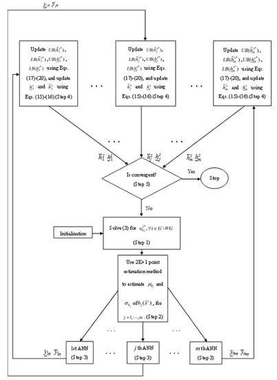
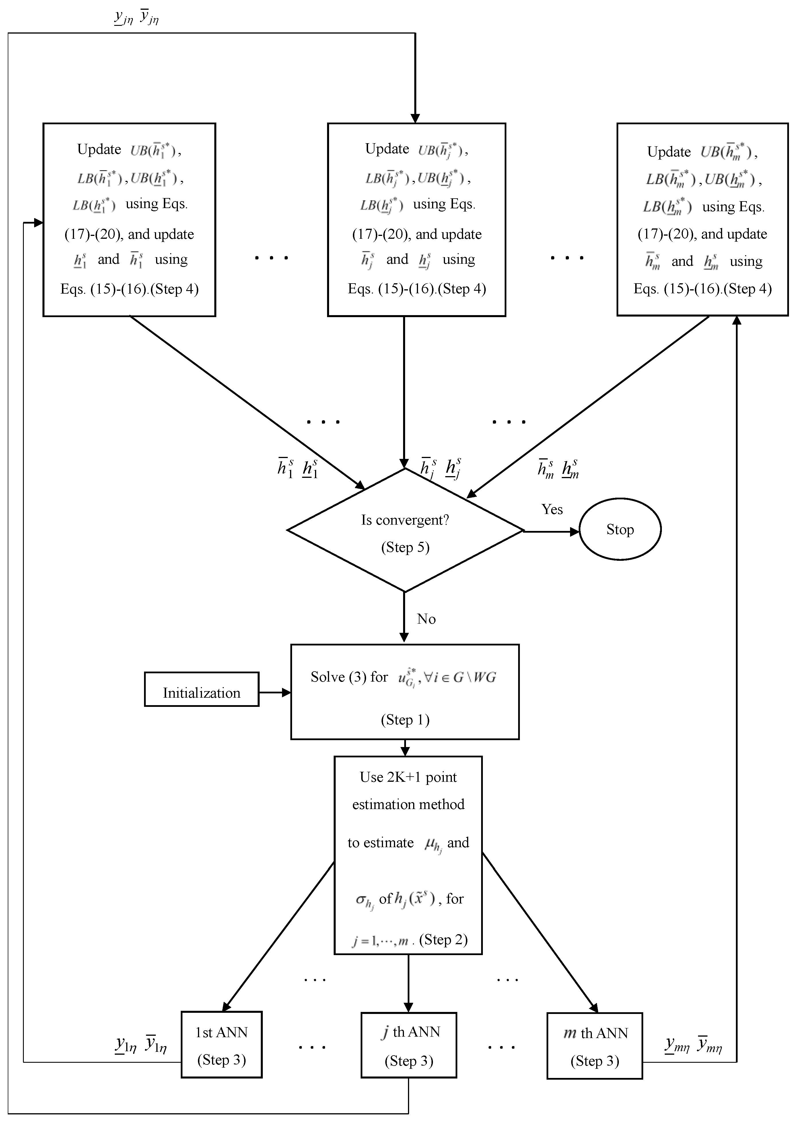
2.2.3. Risk-Limiting Schedule of Optimal Non-Renewable Power-Generation Algorithm

• Initial Setting of Bounds

In the bisection method, the initial values of the four bounds $UB({\overline{h}}_j^{s*})$, $LB({\overline{h}}_j^{s*})$, $UB({\underset{\_}{h}}_j^{s*})$ and $LB({\underset{\_}{h}}_j^{s*})$ must first be specified. With respect to the transmission line real power flow, since ${\overline{h}}_j^o>{\overline{h}}_j^{s*}$, ${\underset{\_}{h}}_j^o=-{\overline{h}}_j^o$ and $|p_{ij}|\ge 0$, the initial values of these four bounds can be set to $UB({\overline{h}}_j^{s*})={\overline{h}}_j^o$, $LB({\overline{h}}_j^{s*})=0$, $UB({\underset{\_}{h}}_j^{s*})=0$ and $LB({\underset{\_}{h}}_j^{s*})={\underset{\_}{h}}_j^o$. With respect to the bus voltage magnitude, since ${\overline{h}}_j^o>{\overline{h}}_j^{s*}>{\underset{\_}{h}}_j^{s*}>{\underset{\_}{h}}_j^o$, the initial values of these four bounds can be set to $UB({\overline{h}}_j^{s*})={\overline{h}}_j^o$, $LB({\overline{h}}_j^{s*})={\underset{\_}{h}}_j^o+d$, $UB({\underset{\_}{h}}_j^{s*})={\overline{h}}_j^o-d$ and $LB({\underset{\_}{h}}_j^{s*})={\underset{\_}{h}}_j^o$, where d is a positive real number.

• Algorithm

Based on the analysis presented in Section 2.2.1 and Section 2.2.2, the algorithmic steps of the proposed RSONP algorithm for solving the RSONP problem (Equation (2)) can be presented in the following.

Given data: The pdf $p(v_l)$, parameters $C_p$, $a$, $A$ and $|\text{cos}{\mathsf{\varphi }}_l|$ of bus $l\in WG$. The pdf $p(P_{D_i^L})$ and $|\text{cos}{\mathsf{\varphi }}_{D_i}|$, $\forall i=1,\cdots ,N^L$. The $m$ ANNs constructed off-line. The values of η, $d$ and ε.

Step 0: Calculate ${\widehat{u}}_{W_l}={[{\widehat{P}}_{W_l},{\widehat{Q}}_{W_l}]}^T$ using Equations (4) and (5) and calculate ${\widehat{u}}_{D_i^L}={[{\widehat{P}}_{D_i^L},{\widehat{Q}}_{D_i^L}]}^T$ using Equation (6) based on $p(v_l)$ and $p(P_{D_i^L})$. For $j=1,\cdots ,m$, set initial values of $UB({\overline{h}}_j^{s*})$, $LB({\overline{h}}_j^{s*})$, $UB({\underset{\_}{h}}_j^{s*})$ and $LB({\underset{\_}{h}}_j^{s*})$ as described above, and calculate ${\overline{h}}_j^s$ and ${\underset{\_}{h}}_j^s$ by Equations (15) and (16).

Step 1: Solve OPFPRB (Equation (3)) using an available OPF solution method [30] and obtain the SONP $u_{G_i}^{s*},\forall i\in G\backslash WG$.

Step 2: Use $2K+1$ point estimation method to estimate ${\mathsf{\mu }}_{h_j}$ and ${\mathsf{\sigma }}_{h_j}$ of $h_j({\tilde{x}}^s)$ for $j=1,\cdots ,m$.

Step 3: For $j=1,\cdots ,m$, input ${\mathsf{\mu }}_{h_j}$ and ${\mathsf{\sigma }}_{h_j}$, obtained in Step 2, into the $j$th ANN, and whose outputs are the estimated η-upper bound ${\overline{y}}_{j\mathsf{\eta }}({\underset{\_}{\mathbf{h}}}^s,{\overline{\mathbf{h}}}^s)$ and η-lower bound ${\underset{\_}{y}}_{j\mathsf{\eta }}({\underset{\_}{\mathbf{h}}}^s,{\overline{\mathbf{h}}}^s)$ of $h_j({\tilde{x}}^s)$.

Step 4: For $j=1,\cdots ,m$, update $UB({\overline{h}}_j^{s*})$, $LB({\overline{h}}_j^{s*})$, $UB({\underset{\_}{h}}_j^{s*})$ and $LB({\underset{\_}{h}}_j^{s*})$ using Equations (17)–(20), and update ${\overline{h}}_j^s$ and ${\underset{\_}{h}}_j^s$ using Equations (15) and (16).

Step 5: If both $UB({\overline{h}}_j^{s*})-LB({\overline{h}}_j^{s*})<\mathsf{\epsilon }{\overline{h}}_j^o$ and $UB({\underset{\_}{h}}_j^{s*})-LB({\underset{\_}{h}}_j^{s*})<\mathsf{\epsilon }{\overline{h}}_j^o$ hold for all $j=1,\cdots ,m$, stop and the final $LB({\overline{h}}_j^{s*})$ and $UB({\underset{\_}{h}}_j^{s*})$ are the solutions for ${\overline{h}}_j^{s*}$ and ${\underset{\_}{h}}_j^{s*}$, respectively, for $j=1,\cdots ,m$; otherwise, return to Step 1. If the algorithm stops, output the optimal restrictive bounds $({\underset{\_}{\mathbf{h}}}^{s*},{\overline{\mathbf{h}}}^{s*})$ and the OSONP $u_{G_i}^{\widehat{s}*},\forall i\in G\backslash WG$, which is obtained from Step 1 in the final iteration.

2.2.4. Flow Chart of the Risk-Limiting Schedule of Optimal Non-Renewable Power-Generation Algorithm

The structure of the proposed RSONP algorithm for solving the RSONP problem can be summarized by the flow chart presented in Figure 2, and the corresponding algorithmic steps are also indicated in the figure.

3. Results and Discussion

3.1. Setup of Tests

The IEEE 118-bus system that is presented in [31] is used as the test system. In this system, there are 44 non-renewable power generation buses, 10 wind power generation buses and 25 buses of large load demand. Consequently, $|WG|=10$, $N^L=25$ and $K=35$. Bus 69 is designated as the swing bus; the number of transmission lines is 186, so $m=304$. $({\underset{\_}{V}}_j^o,{\overline{V}}_j^o)$ and $({\underset{\_}{p}}_{ij}^o,{\overline{p}}_{ij}^o)$ are set to (0.95, 1.05) and $(-|{\widehat{p}}_{ij}|(1+7\%),|{\widehat{p}}_{ij}|(1+7\%))$, respectively, where $|{\widehat{p}}_{ij}|$ is the absolute value of the $p_{ij}$ in the base case. In the OPFPRB (Equation (3)) and COPF problem (Equation (1)), the values of the cost coefficients $a_i,b_i$ and $c_i$ $\forall i\in G\backslash WG$ are randomly selected from the intervals (6.78, 74.33), (8.3391, 37.6968) and (0.002401, 0.069663), respectively. Notably, the units of $a_i,b_i$ and $c_i$ are $/${(\mathrm{MW})}^2{\left(\mathrm{h}\right)}^3$, $/${\mathrm{MW}\left(\mathrm{h}\right)}^2$ and $, respectively. The Weibull distribution given by Equation (22) and the normal distribution given by Equation (23) are adopted for $p(v_l)$ and $p(P_{D_i^L})$, respectively. The parameters used in the RSONP algorithm are set as follows. η = 0.95, $\mathsf{\epsilon }={10}^{-3}$, $d$ = 0.02, $\mathsf{\alpha }=9$, $\mathsf{\beta }=1.6$, $C_p=0.3$, $a=1.225$, $A=706.8$ and $|\text{cos}{\mathsf{\varphi }}_l|$ = 0.9; ${\mathsf{\mu }}_{D_i^L}$ is set to the load demand in the base case, and ${\mathsf{\sigma }}_{D_i^L}$ = 0.03 ${\mathsf{\mu }}_{D_i^L}$. The parameters used in the ANN are set as $q$ = 5 and epochs = 5000.

To study the effect of re-dispatching the SONP $u_{G_i}^{s*}$, $\forall i\in G\backslash WG$, on the performance of the OSONP $u_{G_i}^{\widehat{s}*},\forall i\in G\backslash WG$, and the corresponding generation cost, two test cases, A and B, are designed with extremely different re-dispatching results. In Case A, $r_{P_i}\%=r_{Q_i}\%=0,\forall i\in G\backslash WG$ and $i\ne 69$ are assumed, consistent with a situation in which no non-renewable power generation bus other than the swing bus has a power generation reserve to compensate for the power mismatch. In Case B, $r_{P_i}\%=r_{P_j}\%$ and $r_{Q_i}\%=r_{Q_j}\%,\forall i,j\in G\backslash WG,$ are assumed, approximately consistent with a situation in which all non-renewable power generation buses including the swing bus can generate enough power to compensate for the power deviations of interest.

Notably, all simulations in this test are performed using a personal computer with 3.3 GHz Intel Core I5 and 4 GB RAMS, and all algorithms are implemented in MATLAB (2015b, MathWorks, Natick, MA, USA).

3.2. Test Results, Comparison and Discussions of Case A

Based on the above test setup and the $m$ off-line constructed ANNs, the RSONP algorithm is used to solve the RSONP problems on the IEEE 118-bus system in test Case A to obtain the OSONP $u_{G_i}^{\widehat{s}*},\forall i\in G\backslash WG,$ and the optimal restrictive bounds $({\underset{\_}{\mathbf{h}}}^{s*},{\overline{\mathbf{h}}}^{s*})$. The five Terms (a)–(e) listed in

Table 1. The five terms evaluated in the test. RSONP: risk-limiting schedule of optimal non-renewable power-generation.

Term	Content
(a)	Number of iterations executed in the RSONP algorithm
(b)	Corresponding CPU time of (a)
(c)	${\displaystyle \sum _{j=1}^m[({\underset{\_}{h}}_j^{s*}}-{\underset{\_}{h}}_j^o{)}^2+{({\overline{h}}_j^o-{\overline{h}}_j^{s*})}^2]$
(d)	${\displaystyle \sum _{i\in G\backslash WG}{a}_i(P_{G_i}^{\widehat{s}*}}{)}^2+b_i{P}_{G_i}^{\widehat{s}*}+c_i$
(e)	$\text{Prob}\{{\underset{\_}{h}}_j^o\le h_j({\tilde{x}}^s)\le {\overline{h}}_j^o,\forall j=1,\cdots ,m|{\underset{\_}{\mathbf{h}}}^{s*},{\overline{\mathbf{h}}}^{s*}\}$

are reported or evaluated in this test.

The Terms (a) and (b) correspond to the run time of the RSONP algorithm. Term (c) is the optimal objective value of the RSONP problem (Equation (2)). Term (d) represents the scheduled optimal total non-renewable power generation cost in unit $/h, which is the optimal objective value of the OPFPRB (Equation (3)) when $({\underset{\_}{\mathbf{h}}}^s,{\overline{\mathbf{h}}}^s)=({\underset{\_}{\mathbf{h}}}^{s*},{\overline{\mathbf{h}}}^{s*})$. Term (e) reflects the performance of the OSONP $u_{G_i}^{\widehat{s}*},\forall i\in G\backslash WG,$ and is evaluated based on the MCS presented in Section 2.1.3 but replacing $({\underset{\_}{\mathbf{h}}}^s,{\overline{\mathbf{h}}}^s)$ and $u_{G_i}^{s*},\forall i\in G\backslash WG$ by $({\underset{\_}{\mathbf{h}}}^{s*},{\overline{\mathbf{h}}}^{s*})$ and $u_{G_i}^{\widehat{s}*},\forall i\in G\backslash WG$, respectively.

Table 2. Results of using the RSONP algorithm to solve the RSONP problem on the IEEE 118-bus system in Case A.

(a) *	(b) *	(c) *	(d) *	(e) *
6	48.6	18.292	129,711.75	95.89
7	56.8	10.871	129,699.91	95.74
8	64.5	4.355	129,688.83	95.43
9	72.1	2.871	129,673.23	95.29
10	83.4	0.709	129,661.69	95.21

* Terms regarding (a)–(e) are specified in Table 1.

presents the test results concerning the aforementioned five terms that were obtained using the proposed RSONP algorithm in Case A. Although RSONP algorithm takes ten iterations to reach the termination criterion, the results that were obtained in 6–9 th iterations are also reported. Columns 1 and 3 of Table 2 reveal the iteration-wise improvement of the objective value of the RSONP problem (Equation (2)), indicating that the distance between the obtained restrictive bounds and the normal bounds becomes smaller each iteration. As the restrictive bounds become less restrictive, the scheduled optimal total non-renewable power generation cost shown in Column 4 of Table 2 becomes smaller as predicted. Moreover, as the restrictive bounds becomes more restrictive, the performance of the OSONP $u_{G_i}^{\widehat{s}*},\forall i\in G\backslash WG$, improves but at the cost of an increase in the scheduled optimal total non-renewable power generation cost as is observed from Columns 3–5 in Table 2. This is reasonable, because a higher cost is required for a better performance. The performance of the OSONP $u_{G_i}^{\widehat{s}*},\forall i\in G\backslash WG,$ in iterations six to ten of the RSONP algorithm exceeds 0.95 and the consumed CPU time are all less than 83.4 s, as revealed by Columns 5 and 2 in Table 2. In fact, the RSONP algorithm can be terminated after iteration 7, because the corresponding CPU time is less than one minute, but the performance is 0.55% better than that achieved in ten iterations, at the cost of only a 0.03% increase in the scheduled optimal total non-renewable power generation cost. The above results imply the following. The solution obtained at the end of iteration ten being the best is simply because the objective function of the RSONP problem (Equation (2)) considers only Term (c) that is proportional to Term (d), the non-renewable power generation cost, but do not consider Term (e), the performance regarding the probability of satisfying the security constraints in the presence of uncertain power generation and load demand. Since some system operators may care more about the security than the cost, a multi-objective OPF that considers both non-renewable power generation cost and the probability of satisfying the security constraints would be an issue that is worthy of investigation.

To demonstrate the advantage of the RSONP algorithm, the performance of the obtained OSONP $u_{G_i}^{\widehat{s}*},\forall i\in G\backslash WG,$ is compared with the conventional schedule of optimal non-renewable power-generation (CSONP) $u_{G_i}^{o*},\forall i\in G\backslash WG,$ which is obtained by solving the COPF problem (Equation (1)) using the OPF solution method [30] that was used in Step 1 of the RSONP algorithm. The performance of $u_{G_i}^{o*},\forall i\in G\backslash WG$, is defined as $\text{Prob}\{{\underset{\_}{h}}_j^o\le h_j({\tilde{x}}^o)\le {\overline{h}}_j^o,\forall j=1,\cdots ,m|{\underset{\_}{\mathbf{h}}}^o,{\overline{\mathbf{h}}}^o\}$, where ${\tilde{x}}^o$ is the normal-bound-based random state-vector after re-dispatching (NRSAR) for all buses $i=1,\cdots ,N$. The NRSAR ${\tilde{x}}^o$ is obtained using the procedure that was elucidated in the re-dispatching stage (Section 2.1.3) but with $u_{G_i}^{\widehat{s}*}$, ${\tilde{u}}_{G_i}^s$, $\forall i\in G\backslash WG,$ and ${\tilde{x}}^s$ replaced by $u_{G_i}^{o*}$, ${\tilde{u}}_{G_i}^o$, $\forall i\in G\backslash WG,$ and ${\tilde{x}}^o$, respectively, where ${\tilde{u}}_{G_i}^o,\forall i\in G\backslash WG,$ is the Normal-bound-based Non-renewable Power-generation After Re-dispatching (NNPAR) that was obtained by re-dispatching the CSONP $u_{G_i}^{o*},\forall i\in G\backslash WG,$ using Equations (9) and (10) based on the re-dispatching percentage share in Case A. The procedure for evaluating $\text{Prob}\{{\underset{\_}{h}}_j^o\le h_j({\tilde{x}}^o)\le {\overline{h}}_j^o,\forall j=1,\cdots ,m|{\underset{\_}{\mathbf{h}}}^o,{\overline{\mathbf{h}}}^o\}$ in Case A is also based on the MCS presented in Section 2.1.3 but replacing $({\underset{\_}{\mathbf{h}}}^s,{\overline{\mathbf{h}}}^s)$ and $u_{G_i}^{s*},\forall i\in G\backslash WG$ by $({\underset{\_}{\mathbf{h}}}^o,{\overline{\mathbf{h}}}^o)$ and $u_{G_i}^{o*},\forall i\in G\backslash WG$, respectively. The test results show that the performance of the CSONP $u_{G_i}^{o*},\forall i\in G\backslash WG,$ in Case A is 0.7723 which is far from performance of greater than 0.95 that results from all the OSONP $u_{G_i}^{\widehat{s}*},\forall i\in G\backslash WG,$ obtained in iterations six to ten of the proposed RSONP algorithm as shown in Table 2. However, the total non-renewable power generation cost of $u_{G_i}^{o*},\forall i\in G\backslash WG,$ that is calculated as ${\displaystyle \sum _{i\in G\backslash WG}{a}_i(P_{G_i}^{o*}}{)}^2+b_i{P}_{G_i}^{o*}+c_i$ is $129,630.47/h. Hence, in Case A, the performance of the OSONP $u_{G_i}^{\widehat{s}*},\forall i\in G\backslash WG,$ obtained by executing the RSONP algorithm for ten iterations is 23.28% better than that of CSONP $u_{G_i}^{o*},\forall i\in G\backslash WG,$ at the cost of a 0.024% increase in the total non-renewable power generation cost. The above results reveal that the proposed RSONP algorithm can be applied in real time to a large power system and effectively reduce the risk of violating security constraints in the presence of uncertain power generation and load demand at the very small cost of an increase in the total non-renewable power generation cost.

3.3. Test Results, Comparisons and Discussions of Case B

The procedure of using the RSONP algorithm to solve the RSONP problem on the IEEE 118-bus system in Case B is the same as that in Case A, but with a different re-dispatching percentage share.

Table 3. Results of using the RSONP algorithm to solve the RSONP problem on the IEEE 118-bus system in Case B.

(a) *	(b) *	(c) *	(d) *	(e) *
6	47.5	18.278	129,709.06	95.86
7	56.4	10.843	129,696.38	95.65
8	65.3	4.326	129,681.13	95.38
9	71.5	2.858	129,670.84	95.26
10	82.6	0.722	129,659.72	95.17

* Terms regarding (a)–(e) are specified in Table 1.

presents the test results of Case B regarding the five Terms, (a)–(e), defined in Table 1, and they are qualitatively the same as those in Case A.

To demonstrate the advantage of the RSONP algorithm in Case B, the performance of the previously obtained CSONP $u_{G_i}^{o*},\forall i\in G\backslash WG,$ is also investigated in Case B. The test procedures are the same as that for Case A described in Section 3.2 except for the re-dispatching percentage share. The test result shows that the performance of the CSONP $u_{G_i}^{o*},\forall i\in G\backslash WG,$, i.e., $\text{Prob}\{{\underset{\_}{h}}_j^o\le h_j({\tilde{x}}^o)\le {\overline{h}}_j^o,\forall j=1,\cdots ,m|{\underset{\_}{\mathbf{h}}}^o,{\overline{\mathbf{h}}}^o\}$ in Case B is 0.7715 (<0.95) in contrast to the larger than 0.95 performances resulted from all the OSONP $u_{G_i}^{\widehat{s}*},\forall i\in G\backslash WG,$ obtained by the proposed RSONP algorithm using 6 to 10 iterations as presented in Table 3. Notably, the total non-renewable power generation cost of CSONP $u_{G_i}^{o*},\forall i\in G\backslash WG,$ in Case B is exactly the same as that presented in Case A. Therefore, comparing with the CSONP $u_{G_i}^{o*},\forall i\in G\backslash WG,$ the performance of the OSONP $u_{G_i}^{\widehat{s}*},\forall i\in G\backslash WG,$ obtained from executing the RSONP algorithm for 10 iterations in Case B is 23.35% better at the small cost of a 0.022% increase in the total non-renewable power generation cost. Since the re-dispatching percentage share for all the non-renewable power generation busses in these two cases are extremely different, the test results presented in Table 2 and Table 3 demonstrate the robustness of the proposed RSONP algorithm.

4. Conclusions and Further Research

Intermittent renewable power generation and uncertain load demand may cause security constraints to be violated. To limit this risk, an RSONP problem is formulated and a computationally efficient RSONP algorithm is presented and tested on the IEEE 118-bus power system. The computing speed of the RSONP algorithm and its comparison with the CSONP show that it can be applied in real time to reduce the risk of violating security constraints at the very small cost of an increase in the total non-renewable power generation cost. As for further research, due to the conflicting nature between the non-renewable power generation cost and the probability of satisfying security constraints indicated in Section 3.2, it would be worthwhile to formulate a multi-objective OPF problem by taking into account the aforementioned two conflicting terms and propose a computationally efficient algorithm to solve it.

References

1. Niayifar, A.; Porte-Agel, F. Analytical modeling of wind farms: A new approach for power prediction. Energies 2016, 9, 741. [Google Scholar] [CrossRef]
2. Cho, Y.; Lee, C.; Hur, K.; Kang, Y.C.; Muljadi, E.; Park, S.-H.; Choy, Y.-D.; Yoon, G.-G. A framework to analyze the stochastic harmonics and resonance of wind energy grid interconnection. Energies 2016, 9, 700. [Google Scholar] [CrossRef]
3. Curreli, A.; Serra-Coch, G.; Isalgue, A.; Crespo, I.; Coch, H. Solar energy as a form giver for future cities. Energies 2016, 9, 544. [Google Scholar] [CrossRef]
4. Buonomano, A.; Calise, F.; Vicidomini, M. Design, simulation and experimental investigation of a solar system based on PV and PVT collectors. Energies 2016, 9, 496. [Google Scholar] [CrossRef]
5. Luo, Z.; Hong, S.-H.; Kim, J.-B. A price-based demand response scheme for discrete manufacturing in smart grids. Energies 2016, 9, 650. [Google Scholar] [CrossRef]
6. Kim, Y.-S.; Hwang, C.-S.; Kim, E.-S.; Cho, C. State of charge-based active power sharing method in a standalone microgrid with high penetration level of renewable energy sources. Energies 2016, 9, 480. [Google Scholar] [CrossRef]
7. Li, Y.; Li, W.; Yan, W.; Yu, J.; Zhao, X. Probabilistic optimal power flow considering correlations of wind speeds following different distributions. IEEE Trans. Power Syst. 2014, 29, 1847–1854. [Google Scholar] [CrossRef]
8. Zou, B.; Xiao, Q. Solving probabilistic optimal power flow problem using quasi Monte Carlo method and ninth-order polynomial normal transformation. IEEE Trans. Power Syst. 2014, 29, 300–306. [Google Scholar] [CrossRef]
9. Dvorkin, Y.; Pandzic, H.; Ortega-Vazquez, M.A.; Kirschen, D.S. A hybrid stochastic/interval approach to transmission-constrained unit commitment. IEEE Trans. Power Syst. 2015, 30, 621–631. [Google Scholar] [CrossRef]
10. Wu, H.; Shahidehpour, M.; Li, Z.; Tian, W. Chance-constrained day-ahead scheduling in stochastic power system operation. IEEE Trans. Power Syst. 2014, 29, 1583–1591. [Google Scholar] [CrossRef]
11. Ahmadi-Khatir, A.; Conejo, A.J.; Cherkaoui, R. Multi-area unit scheduling and reserve allocation under wind power uncertainty. IEEE Trans. Power Syst. 2014, 29, 1701–1710. [Google Scholar] [CrossRef]
12. Kusiak, A.; Verma, A.; Wei, X. Wind turbine capacity frontier from SCADA. Wind Syst. Mag. 2012, 3, 36–39. [Google Scholar]
13. Sttt, B.; Marinho, J.L. Linear programming for power system network security applications. IEEE Trans. Power Appl. Syst. 1979, 98, 837–848. [Google Scholar] [CrossRef]
14. Burchett, R.C.; Happ, H.H.; Vierth, D.R. Quadratically convergent optimal power flow by Newton approach. IEEE Trans. Power Appl. Syst. 1985, 103, 3267–3275. [Google Scholar]
15. Sun, D.I.; Ashly, B.; Brewer, B.; Hughes, A.; Tinney, W.F. Optimal power flow by Newton approach. IEEE Trans. Power Appl. Syst. 1984, 103, 2864–2880. [Google Scholar] [CrossRef]
16. Wu, Y.; Debs, A.S.; Marsten, R.E. A direct nonlinear predictor-corrector primal-dual interior point algorithm for optimal power flow. IEEE Trans. Power Syst. 1994, 9, 876–882. [Google Scholar]
17. Lin, C.-H.; Lin, S.-Y. A new dual-type method used in solving optimal power flow problems. IEEE Trans. Power Syst. 1997, 12, 1667–1675. [Google Scholar]
18. Salgado, R.S.; Ranger, E.L., Jr. Optimal power flow solutions through multi-objective programming. Energy 2012, 42, 35–45. [Google Scholar] [CrossRef]
19. Narimani, M.R.; Azizipanah-Abarghooee, R.; Zoghdar-Moghadam-Shahrekohne, B.; Gholami, K. A novel approach to multi-objective optimal power flow by a new hybrid optimization algorithm considering generator constraints and multi-fuel type. Energy 2013, 49, 119–136. [Google Scholar] [CrossRef]
20. Niknam, T.; Narimani, M.R.; Jabbari, M.; Malekpour, A.R. A modified shuffle frog leaping algorithm for multi-objective optimal power flow. Energy 2011, 36, 6420–6432. [Google Scholar] [CrossRef]
21. Niknam, T.; Azizipanah-Abarghooee, R.; Narimani, R. Reserve constrained dynamic optimal power flow subject to valve-point effects, prohibited zones and multi-fuel constraints. Energy 2012, 47, 451–464. [Google Scholar] [CrossRef]
22. Varaiya, P.; Wu, F.F.; Bialek, J.W. Smart operation of smart grid: Risk-limiting dispatch. Proc. IEEE 2011, 99, 40–57. [Google Scholar] [CrossRef]
23. Zhang, H.; Li, P. Chance constrained programming for optimal power flow under uncertainty. IEEE Trans. Power Syst. 2011, 26, 2417–2424. [Google Scholar] [CrossRef]
24. Lin, S.-Y.; Lin, A.-C. RLOPF (risk-limiting optimal power flow) for systems with high penetration of wind power. Energy 2014, 71, 49–61. [Google Scholar] [CrossRef]
25. Danaraj, R.M.S. Economic Dispatch by Quadratic Programming. Available online: http://www.mathworks.com/matlabcentral/fileexchange/19538-economic-dispatch-by-quadratic-programming (accessed on 4 April 2015).
26. Svozil, D.; Kvasnicka, V.; Pospichal, J. Introduction to multi-layer feed-forward neural networks. Chemom. Intell. Lab. Syst. 1997, 39, 43–62. [Google Scholar] [CrossRef]
27. Wei, X.; Kusiak, A.; Sadat, H.R. Prediction of influent flow rate: Data-mining approach. J. Energy Eng. 2012, 139, 118–123. [Google Scholar] [CrossRef]
28. Wilamowski, B.M.; Yu, H. Improved computation for Levenberg-Marquardt training. IEEE Trans. Neural Netw. 2010, 21, 930–937. [Google Scholar] [CrossRef] [PubMed]
29. Morales, J.M.; Perez-Ruiz, J. Point estimate schemes to solve the probabilistic power flow. IEEE Trans. Power Syst. 2007, 22, 1594–1601. [Google Scholar] [CrossRef]
30. Zimmerman, R.; Murillo-Sanchez, C.; Gan, D. MATPOWER: A MATLAB Power System Simulation Package; PSERC, Cornell University: Ithaca, NY, USA, 2005. [Google Scholar]
31. IIT Power Group. One-Line Diagram of IEEE 118-Bus System. Illinois Institute of Technology, 2003. Available online: http://motor.ece.iit.edu/data/IEEE118bus_inf/IEEE118bus_figure.pdf (accessed on 25 May 2015).
Figure 1. Three-layer artificial neural network (ANN).
Energies 09 00868 g001
Figure 2. Flow chart of the risk-limiting schedule of optimal non-renewable power-generation algorithm.
Energies 09 00868 g002