Article

Operational Modal Analysis of a Spar-Type Floating Platform Using Frequency Domain Decomposition Method

1
Natural Ocean Engineering Laboratory (NOEL), Mediterranea University of Reggio Calabria, Reggio Calabria 89122, Italy
2
DICEAM Department, Mediterranea University of Reggio Calabria, Reggio Calabria 89122, Italy
3
Energy and Power Department, Cranfield University, Cranfield MK43 0AL, UK
4
Tecnalia Research & Innovation, Energy and Environment Division, Bilbao 48160, Spain
*
Author to whom correspondence should be addressed.
Energies 2016, 9(11), 870; https://doi.org/10.3390/en9110870
Submission received: 21 July 2016 / Revised: 19 September 2016 / Accepted: 17 October 2016 / Published: 26 October 2016
(This article belongs to the Special Issue Modeling and Simulation for Wind Turbine Loads Analysis)

Abstract

:
System identification of offshore floating platforms is usually performed by testing small-scale models in wave tanks, where controlled conditions, such as still water for free decay tests, regular and irregular wave loading can be represented. However, this approach may result in constraints on model dimensions, testing time, and costs of the experimental activity. For such reasons, intermediate-scale field modelling of offshore floating structures may become an interesting as well as cost-effective alternative in a near future. Clearly, since the open sea is not a controlled environment, traditional system identification may become challenging and less precise. In this paper, a new approach based on Frequency Domain Decomposition (FDD) method for Operational Modal Analysis is proposed and validated against numerical simulations in ANSYS AQWA v.16.0 on a simple spar-type structure. The results obtained match well with numerical predictions, showing that this new approach, opportunely coupled with more traditional wave tanks techniques, proves to be very promising to perform field-site identification of the model structures.

1. Introduction

Floating wind turbine concepts have been actively investigated in the last decades. Theoretical and experimental studies have recently demonstrated technical feasibility and economic benefits of floating concepts in waters deeper than 50–60 m, where standard fixed supports are not feasible or too expensive [1,2,3,4,5,6]. Among floating concepts under study, the spar, consisting of a slender hollow cylinder, placed in vertical position and ballast-stabilized, seems to be particularly appropriate for deep waters (above 100 m). Spar prototypes are involved in projects such as UMaine-Hywind [4], Hywind [7], and OC3-Hywind [8,9]. Insight into the wind-wave response of a spar floating wind turbine has been provided by numerical studies—see e.g., Karimirad and Moan [10].
Experimental tests play a crucial role in the development and assessment of floating wind turbines. For inherent difficulties in full scale testing, tests on scale models are generally conducted, either in seawater or, more frequently, in wave basins or tanks [11,12,13,14]. In particular, field experiments in seawater allow the use of intermediate to large scale models, better representing the key features of the full scale structure, although the non-controlled environment may prove the interpretation of the results to be more challenging. With regard to spar concepts only, comparisons between experimental and numerical results have been carried out by Sethuraman and Venugopal [11] on a scale wind turbine mounted on a stepped spar using OrcaFlex, Skaare et al. [12] on a 1:47 scale model of the Hywind spar using SIMO/RIFLEX, and Myhr et al. [13] on a scale model of OC3-Hywind spar using 3Dfloat and ANSYS. A 1:128 scale model of OC3-Hywind with three catenary mooring lines has been realized and tested by Shin [14], under periodic waves and irregular waves. The authors are currently investigating a 1:30 scale model of the OC3-Hywind spar in seawater, installed at the NOEL laboratory of Reggio Calabria, Italy [15].
Since floating supports for offshore wind turbines can often be treated as rigid bodies, the most common approach in the investigation of their dynamic behavior is based on six degrees of freedom models, processed in time or frequency domain to figure out the main dynamic characteristics on the structure with respect to the standard motions of surge, sway, heave, roll, pitch, and yaw. However, often, motions in different degrees of freedom are coupled and it makes sense to adopt modal analysis to achieve a deeper understanding of the system rigid body dynamics. In this context, experimental system identification may be attempted also in non-controlled environments using Operational Modal Analysis (OMA) methods, which make use of structural response data only, under the assumption that the input can be taken as white noise, or random excitation with broadband frequency content over the range of structural natural frequencies. This is frequently the case in engineering structures like buildings, towers, bridges, and offshore structures, loaded by ambient forces like wind, waves, or traffic. Examples of OMA methods are Stochastic Subspace Identification (SSI) method, Peak-Picking (PP) method, Frequency Domain Decomposition (FDD) method, Ibrahim Time-Domain (ITD) method, Eigensystem Realization Algorithm (ERA), Random Decrement Technique (RDT) [16,17,18].
These techniques have been applied to offshore structures in a few studies. Park et al. [19] have identified natural frequencies and corresponding mode shapes of a scale steel box structure floating in a water tank, using the FDD method in conjunction with the PP method. They assessed the correlation between experimental and analytical modal parameters built by a finite element model. Liu et al. [20] applied the SSI method to a real four-leg jacket-type offshore platform located in China. Kim et al. [21] identified the mode shapes of a segmented hull model towed in a model basin using RDT and Proper Orthogonal Decomposition (POD). Mysolzyk et al. [22] applied the FDD method to identify a scale tripod model in a wave basin.
All the above-mentioned studies refer to the structural vibration analysis (elasticity), while operational modal analysis has never been used to identify the coupled rigid body motion of a floating structure. Within the research activities currently carried out by the authors on a 1:30 scale model of the OC3-Hywind prototype at the NOEL laboratory [15], this paper aims to assess the feasibility of a FDD approach to identify an ANSYS-AQWA [23] numerical implementation of a spar structure, under irregular waves generated by JONSWAP spectrum. Natural frequencies, mode shapes, and modal damping ratios are obtained for different parameters of JONSWAP spectrum. Numerical results show that a FDD approach does provide sufficiently accurate results when the peak of the JONSWAP spectrum is relatively far from the natural frequencies of the spar, because in this case the input excitation is pretty flat in the range of interest. On the contrary, accuracy deteriorates as the natural frequencies fall at the vicinity of the peak, due to the relevant steepness of the spectral function in this range.
The paper is organized as follows: the basic principles of FDD method are illustrated in Section 2, the numerical model of the spar is described in Section 3, and the results of the FDD identification are discussed in Section 4.

2. Frequency Domain Decomposition (FDD) Method

A complete analytical treatment of the FDD method is out of the scope of this work. In this section, the main hypotheses are highlighted and a brief overview is given. A more detaileddescription of the method can be found in Brincker et al. [17,18].

2.1. Hypotheses of the Method

Frequency Domain Decomposition (FDD) is a non-Bayesian method for Operational Modal Analysis of structures. Acting in the frequency domain, it gives the mode shapes and the associated natural frequencies and damping coefficients as output, given a sufficient number of measurement channels as input. The most important requirements of the method are the following:
  • The equations of motion of the structure are linear.
  • The structure is lightly damped, e.g., modal damping coefficients do not exceed 10%–15%.
  • The external load on the structure, though unknown, can be regarded as a white noise over the frequency range of interest.
In view of an application of the method for the dynamic identification of rigid body motions of offshore structures, the first hypothesis can be considered fulfilled whenever potential theory holds or non-linear terms, such as viscous drag damping on slender cylinders, can be reasonably linearized (see e.g., Chakrabarti [24], Spanos [25]). Provided that the equation of motion has been expressed in an appropriate linear form, the second assumption may be considered as valid in several applications of interest. Whenever damping is high, due to sea state severity or structural characteristics, FDD method should not be adopted. Regarding the third hypothesis, ocean wave spectra are typically narrow-banded, hence the applicability of the FDD technique for system identification of offshore structures in real seas is questioned. The aim of the present work is to investigate the applicability and the efficiency of the FDD method on offshore structures, under common operational conditions driven by JONSWAP spectra [26], in view of possible future applications of the method to field experiments.

2.2. Brief Overview of the Method

Generally, the dynamics of a structure can be described by an infinite number of degrees of freedom; however, in engineering practice, structure motions are usually represented by a finite number of variables, usually translations or rotations, kept as low as possible to make analysis simpler. In the case of offshore structures, one can often treat the structure as a single rigid body resulting in only six degrees of freedom corresponding to the rigid translations and rotations of the structure.
If the equation of motion of the structure is linear, its response in terms of motion y(t) can always be seen as a linear combination of the modal contributions:
y ( t ) = Φ q ( t )
where Φ is the mode shape matrix and q(t) the set of modal coordinates. Straightforwardly, the covariance matrix Cyy(τ) of the response y is related to the covariance matrix Cqq(τ) of the modal coordinates q as shown in Equation (2). By taking Fourier Transform of both sides of Equation (2), we obtain the relation between the two power spectral matrices Syy(ω) and Sqq(ω), shown in Equation (3).
C y y ( τ ) = Φ C q q ( τ ) Φ T
S y y ( ω ) = Φ S q q ( ω ) Φ T
Under the assumption of uncorrelated modes [16], it must be noted that, for any fixed frequency, Equation (3) is formally equivalent to a Singular Value Decomposition (SVD) of the spectral density matrix Syy, being Sqq a diagonal matrix. In detail, each column of the mode shape matrix Φ represents a singular vector and each corresponding term in the main diagonal of Sqq is the corresponding singular value. The order of the singular vectors at each frequency ω depends on that of singular values, which are conventionally sorted in descending order.
The practical application of the FDD method descends directly from the few considerations above. In fact, given a certain number of measurement channels on the structure, equal to or larger than the number of modes used to represent the structure motions, one can easily calculate the power spectral matrix Syy(ω). Then, for each frequency ω, the matrix Φ(ω) and the diagonal matrix Sqq(ω) can be obtained through SVD.
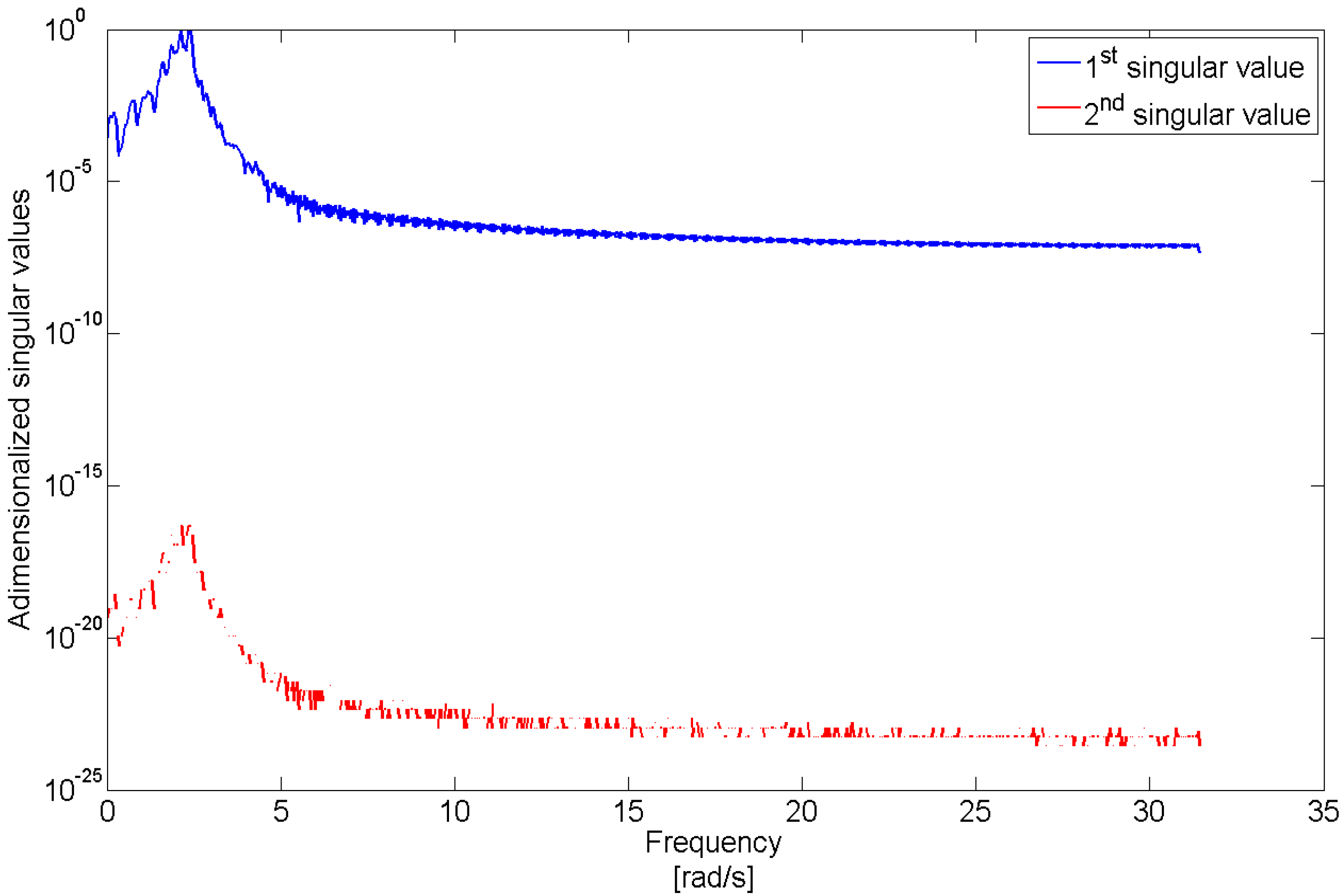
For instance, considering an ideal 2-Degrees Of Freedom (DOF) system, a typical plot of the two singular values in the frequency domain will be like that of Figure 1.
At the natural frequency ωn,i of the i-th mode, the spectral density matrix Syyn,i) will be dominated by that mode. As a consequence, due to Equation (3) and to the fact that singular values of SVD are sorted in descending order, the first term of the diagonal matrix Sqqn,i) will represent the modal spectral density ordinate of the mode at its natural frequency, and the first column of the matrix Φn,i) will represent the mode shape vector. The two peaks of the first singular value plot in Figure 1 occur each at the natural frequency of a mode and represent the corresponding modal spectral density ordinates at that frequency.
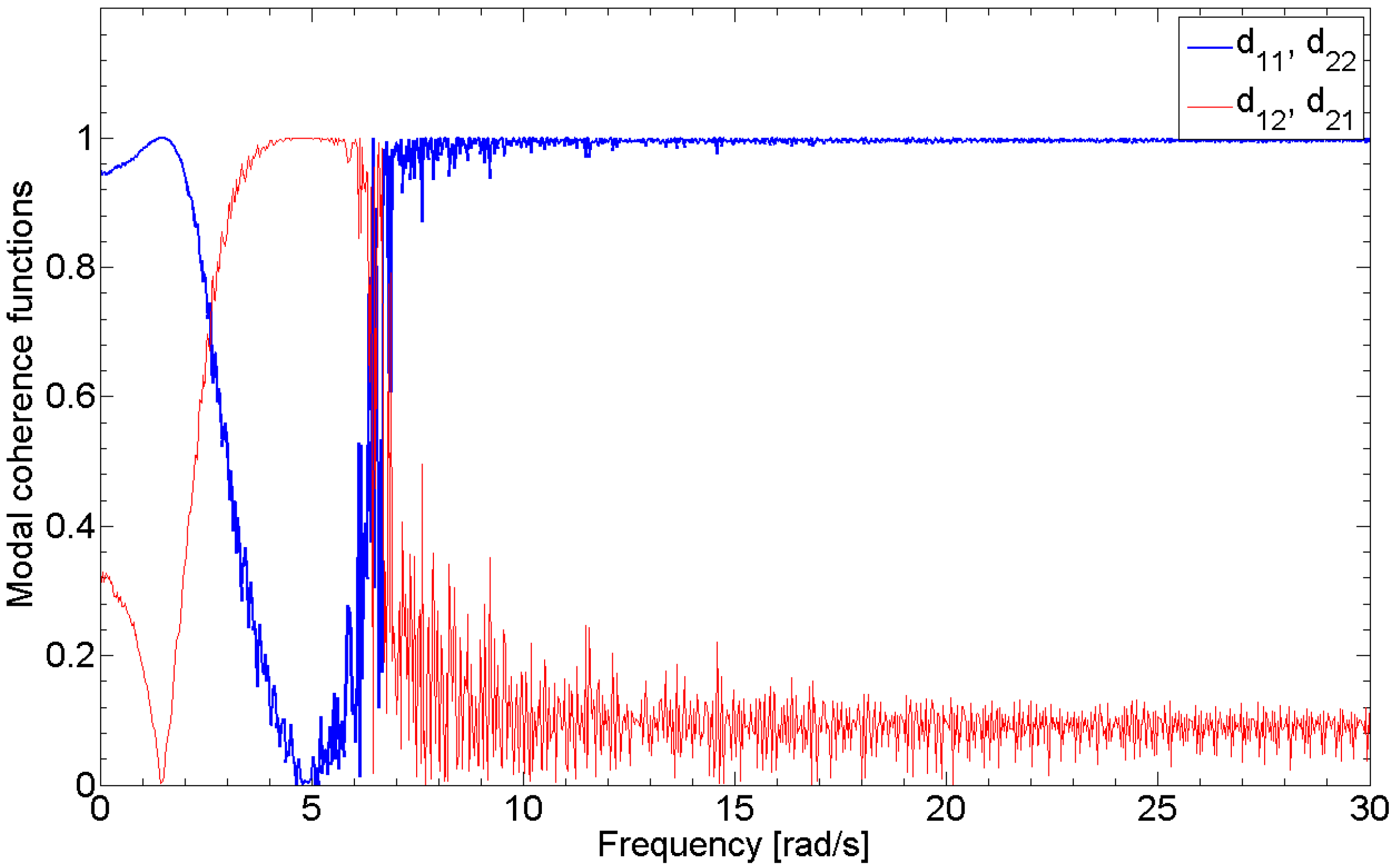
In order to estimate over the whole frequency domain the two modal spectral density functions, which will be used for the estimation of the modal damping, mode shape can be used to define a discrimination function, referred to as modal coherence. Practically speaking, the modal coherence of the mode j with respect to the mode k is a function of frequency defined as:
d j k ( ω ) = | φ j ( ω ) φ k ( ω n , k ) | ,
The modal coherence functions of the two singular vectors of the ideal case represented in Figure 1, with respect to the two mode shapes of the system, are shown in Figure 2.
The modal coherence function allows us to define a similarity criterion between the mode shape vector and the singular vectors estimated at all the frequencies. In fact, the value of the modal coherence tends to unity as the singular vector estimation tends to the mode shape. As a consequence, we can arbitrarily define a threshold sufficiently close to unity and assume that the singular vector calculated at each frequency actually corresponds to a mode shape if the corresponding modal coherence exceeds this threshold:
φ j ( ω ) φ k d j k ( ω ) > t 2 ,
Straightforwardly, we can build the modal power spectral density function for each estimated mode, as:
S j ( ω ) = S q k , q k ( ω ) d j k ( ω ) > t 2 ,
It should be noted that Equation (6) is referred to the whole frequency domain, hence the modal power spectral density function can be estimated for a wide frequency range, including frequencies far from the modal natural frequency. However, there may be some small regions in the frequency domain where the modal coherence of all the modes is less than the threshold t2 (see e.g., the frequencies around 2.5 rad/s in Figure 2). These regions correspond to the frequency values where the singular vectors switch from a structural mode to another. According to Equation (6), it is theoretically not possible to estimate modal spectral density in these regions. However, provided that the choice of the threshold t2 is appropriate, these regions are very narrow and sufficiently far from the modal natural frequency, resulting in relatively small spectral density ordinates. As a consequence, the damping estimation is not significantly affected by the presence of these regions and so the modal spectral density can be accepted as it is or, equivalently, corrected—e.g., by linear interpolation.
Many engineering applications fall in a case similar to that of Figure 1—i.e., each mode dominates structure dynamics at its natural frequency. Alternatively, there may be cases—e.g., dealing with certain offshore structures—in which some additional issues are to be tackled since there are modes which do not dominate the structure dynamics at their natural frequency. A very common case in offshore engineering is given by structures whose different modes have approximately the same natural frequency, due to the symmetrical nature of the structures. In this case, depending on the excitation forces and on the system damping, near the natural frequency of these modes, one of them will be dominating over the others. As a consequence, the first entry of the matrix Sqq at the natural frequency of these modes will represent the modal spectral ordinate of the dominating mode and the first column of the matrix Φ will represent its mode shape, while the information related to the non-dominating mode will be shifted to the subsequent positions in the matrices. This case is schematically represented in Figure 3, always dealing with an ideal 2-DOF system.
A similar situation may occur also when a mode is dominating the structure dynamics over a wide frequency range, to the extent that it overwhelms other modes at their natural frequencies, even if they are relatively far from the natural frequency of the dominating mode. From a physical point of view, this situation may occur when one mode contribution to the overall structure response is very low, either because of the characteristics of the structure or of the external load. However, this may also happen for numerical reasons when the variables in Syy have different measurement units. That is the case, for example, of structures whose degrees of freedom are translational and rotational, as it is typical in offshore practice where the structures are regarded as rigid bodies. In such cases the choice of measurement units—e.g., degrees or radians—dramatically affects the numerical importance of one mode among the others, so that one class of motions may numerically overwhelm the other, occupying the first entries of the matrices. Theoretically speaking, the final result of the method is not affected by that choice since only the positions of the different contributions in the SVD matrices vary, while identified mode shapes, natural frequencies, and modal spectral density functions should remain the same. However, in practice, attention should be paid to avoid overwhelmed modes, since results are less accurate in the last entries of the matrix.
To summarize the above discussion, FDD method is based on the correct interpretation of the coupled information coming from the singular value plot and the modal coherence function for each singular vector. It is important to remark that, in the most general case, the “horizontal reading” of the first singular value in the singular value plot may not be sufficient to identify all the peaks related to each mode and that a “vertical reading” may be also needed, not only to identify the possibly missing peaks in the first singular value—as it happens e.g., in Figure 2—but also to reconstruct the modal spectral density function of each mode in the entire frequency domain, including frequencies far from its natural one.
Once the modal spectral density function is estimated for each mode, damping ratio can be estimated too using classical methods such as the half power bandwidth method, which acts directly on the modal power spectral density in the frequency domain, or the logarithmic decrement, which acts on the modal auto-correlation—i.e., the Inverse Fourier Transform of the modal power spectral density—in the time domain. The latter is usually more accurate, hence it has been chosen for the present study.

3. Case Study

3.1. Description of the Numerical Model of the Structure

The structure chosen for the present work is a moored spar, inspired to the OC3-Hywind Spar buoy coupled with the NREL-5MW offshore wind turbine in fully parked conditions [9].
The ANSYS AQWA software package has been used for the numerical modeling of the structure response. The hull has been represented using 104 line elements and wave forces have been calculated by means of Morison Equation:
f = f I n + f D r ,
f I n = ( 1 + c A ) ρ π R 2 a w c A ρ π R 2 u ¨ ,
f D r = c D ρ R | v w u ˙ | ( v w u ˙ ) ,
where aw and vw represent respectively the wave particle velocity and acceleration, u the vector of element motions, R the radius of the line element, ρ the water density, and cA and cD the added mass and drag coefficients.
The nonlinear term in Equation (7) represents a drag viscous damping, which is the main source of damping for spar structures. However, as shown e.g., in Jonkman [9], experimental evidence on spar structures often reveals the presence of some additional linear damping that cannot be regarded neither as viscous nor as radiation damping. Consequently, linear damping matrices are usually added to better represent the structure response.
The aim of this work is to test, for the first time, the applicability and the efficiency of the FDD technique in the non-controlled offshore environment. Therefore, instead of considering the linearized damping coefficient of the OC3-Hywind, augmented by the additional damping suggested by Jonkman [9], a wide range of reference values has been considered for the modal damping coefficients. These values have been chosen as those that would be reasonably encountered in typical offshore structures upon applying a linearization procedure, and span the whole range of damping levels allowed by the FDD method, as mentioned in Section 2.1. The added mass coefficient cA has been set equal to 1.0.
Table 1 and Table 2 respectively report the main characteristics of the structure and of its mooring system, which is made up of three equally spaced catenary lines.

3.2. Modal Analysis of the Structure

Except for the nonlinear restoring from mooring lines, which is revealed to be negligible in the range of motions considered in this work, the system dynamics is fully linear. Consequently, modal analysis of the structure is expected to give the same results as the FDD method applied to the time histories of the structure motions.
In order to perform the modal analysis of the structure, all the elements of the mass matrix have been obtained as the sum of the structural mass or inertia and the corresponding added mass, calculated by means of Equation (8) as:
A 11 = z min 0 c A ρ π R 2 ( z ) d z ,
A 15 = A 51 = z min 0 c A ρ π R 2 ( z ) ( z z G ) d z ,
A 55 = z min 0 c A ρ π R 2 ( z ) ( z z G ) 2 d z ,
The stiffness matrix has been obtained by calculating separately the hydrostatic terms relative to the motions of heave, roll, and pitch and the mooring terms relative to surge and sway, using catenary equation. The yaw term has been assumed equal to that suggested by Jonkman [9] for the OC3-Hywind.
The resulting non-zero terms of mass and stiffness matrices of the structure are reported in Table 3. The natural frequencies and the normalized mode shape vectors of the structure, calculated by means of classical modal analysis, are reported respectively in Table 4 and in Equation (13), where translations are expressed in meters, and rotations in radians. In the following, modes will always be referred to as ordered in Table 4 and Equation (13).
Φ = [ α γ β γ 0 α δ β δ 0 β γ α γ 0 β δ α δ 0 0 0 1 0 0 0 4.5 × 10 4 β γ 4.5 × 10 4 α γ 0 1.1 × 10 1 β δ 1.1 × 10 1 α δ 0 4.5 × 10 4 α γ 4.5 × 10 4 β γ 0 1.1 × 10 1 α δ 1.1 × 10 1 β δ 0 0 0 0 0 0 1 ] ,
where the non-dimensional real variables (γ, δ) represent the normalization factors of the mode shapes. Since the structure is axisymmetric, two eigenvalues (natural frequencies) have multiplicity 2 (see Table 4), hence the corresponding eigenvectors (mode shapes) depend on two arbitrary parameters (α, β). In our case, these parameters are taken as coincident with the load direction. Assuming that the wave direction is identified by the angle θ with respect to x-direction, we can use:
α = cos θ ; β = sin θ ,

4. Results of the FDD Technique

In this section, the results of the FDD technique are presented and commented. Four damping combinations are used to represent a wide range of possible structure designs. In the two sub-sections, two wave spectra are considered: the first one is typical of the operational conditions of the structure at the full scale, while the second one is close to the resonant frequency of some modes, a situation in which the identification method is expected to fail.

4.1. Non-Resonant Wave Conditions

The motions of the structure subjected to a sea state, representative of common operational conditions, have been obtained in ANSYS AQWA for four different cases, setting damping ratios of each mode in a way that a wide range of damping matrices, corresponding to lightly, moderately, and strongly damped structures is investigated.
Each analysis has a duration of 20,000 s and a time step of 0.4 s. The sea state chosen for the four analyses has significant wave height of 2 m, peak frequency of 1 rad/s and JONSWAP spectrum. It should be noted that the peak of the wave spectrum is sufficiently far from the natural frequencies of the spar structure, except that of yaw motion. Consequently, the values of the spectrum in the range of the natural frequencies is almost constant and equal to 0. The sample frequency is variable from 0.005 rad/s close to the structure natural frequencies to 0.1 rad/s close to the peak of the spectrum. The wave direction is set equal to 45°.
The modal shape matrix of the structure for the case study considered is shown in Equation (15), where degrees are chosen among radians as the measurement unit of rotations, due to the numerical issues mentioned in Section 2.2, while translations are expressed in meters. The damping ratios chosen for each of the four cases are reported in Table 5.
Φ = [ 0.707 0.707 0 0.115 0.115 0 0.707 0.707 0 0.115 0.115 0 0 0 1 0 0 0 0.018 0.018 0 0.698 0.698 0 0.018 0.018 0 0.698 0.698 0 0 0 0 0 0 1 ] ,
Damping matrices have been obtained for each case and motions of the structure have been figured out using ANSYS AQWA. Then, FDD analysis has been run, using a built-in code, and results have been compared in terms of natural frequencies, damping ratios, and mode shapes, using the modal coherence as defined in Equation (4), between the mode shapes resulting from modal analysis and those estimated from FDD. The value chosen for the threshold t2 mentioned in Equations (5) and (6) is 0.85.
The singular value plot obtained in the first case is shown in Figure 4 to illustrate a typical output of the method for the case study considered.
The first singular value has three peaks. The first two correspond respectively to the first and the third mode, while the third one corresponds to the JONSWAP spectrum (it has been smoothed to overcome the coarse discretization realized in AQWA in the frequency domain). As expected, the first singular value does not show the peaks relative to all the six modes, since the natural frequencies of the missing modes are close to those already identified. It is thus necessary to read the plot “vertically”, passing to the subsequent singular values. In particular, the second singular value shows the peak relative to the fourth mode and the third singular value shows the peaks relative to the second and the fifth modes. It should be noted that the small peak, which can be observed in the second singular value at low frequencies does not correspond to any real mode but represents a “transition” between the real ones.
The sixth mode, which is limited to the yaw motion, cannot be estimated properly because the simplified numerical model of the structure does not take into account any wave force in this degree of freedom. However, a small peak corresponding to the sixth mode can be observed in the third singular value plot at the frequency of about 0.3 rad/s, corresponding to a minor peak in the Response Amplitude Operator of the structure in yaw, estimated by AQWA at almost the same frequency. As a consequence, the sixth mode shape has been successfully estimated, while the information on the natural frequency and the damping ratio are not sufficient to obtain an accurate estimation.
As it can be seen, the singular value plot is itself a precious source of information on the dynamic behavior of the structure. From a more quantitative point of view, the efficiency of the FDD technique in the four cases of the present study is shown in terms of comparison between input data and output of FDD in Table 6, Table 7, Table 8 and Table 9.
Except for the sixth mode, which has already been discussed, the results of the identification are quite satisfactory. In terms of natural frequencies, we have a little underestimation respect to the input data, but errors never exceed 15%. Regarding mode shapes, the identification is almost perfect except for some rare cases, when the mode is identified using the lowest singular values. This is the case of the second mode in the fourth case, which has been identified through the fourth singular vector. Damping estimations are very good for the dominating modes—i.e., the first and the third—which are always identified through the first singular vector, while they become poorer when using the lower singular vectors. However, it should be kept in mind that, in real applications, the damping matrix often does not have an evident physical meaning and is usually defined in a conventional way to take into account multiple effects. As a consequence, the estimation of FDD technique, though approximate, can be regarded as a useful mean to obtain information about structure damping at least in its order of magnitude.

4.2. Close to Resonance Wave Conditions

The same process of Section 4.1 has been attempted shifting the peak frequency of the wave spectrum to 0.3 rad/s, which is close to the natural frequencies of the third, fourth and fifth mode, as well as to the pseudo-peak of the sixth mode. All the other parameters are kept the same.
The singular value plot is shown in Figure 5 for the first combination of damping ratios, which is the only one considered in this case.
As it can be seen, in this case, the peak relative to the first mode is still clearly identified by the first singular value, while the one relative to the third mode cannot be figured out, since it lies in the range of JONSWAP spectrum. Similarly, the third and the fourth mode cannot be clearly identified. It is interesting to note, however, that the “transitional” peak of the second singular value at low frequency observed in Figure 4 is not present in Figure 5. That happens because the almost resonant modes (third, fourth, and fifth) limit their influence on the first two singular values to the frequency range interested by resonance. As a consequence, the peak in the second singular value at low frequency in this case corresponds to the second mode, enabling it to be identified more accurately than previously, when it fell in the third singular value. At last, it is remarkable that the pseudo-peak in the third singular value—corresponding to the sixth mode—is still present in the singular value plot, even if its frequency is closer to the peak frequency of the wave spectrum than the ones of the other almost resonant modes. The physical reason of this permanence is that, as it has been mentioned previously, no wave force in yaw degree of freedom is taken into account in the mode, hence the wave does not provoke resonance. The quantitative results of the identification process are reported in Table 10.
As evident from Figure 5, the estimations for third, fourth, and fifth mode are not reliable in such a case, while the first two modes are described even more accurately than in Section 3.1 and the sixth mode shape is still estimated correctly.

5. Conclusions

The present work proposes a methodology for the dynamic identification of the rigid body motions of a spar floating support for offshore wind turbine, using the Frequency Domain Decomposition (FDD) method for Operational Modal Analysis. The method has been applied on a numerical model of the spar floating support, implemented in ANSYS AQWA, where the rotor is assumed to be in fully parked conditions and the rotor-nacelle assembly is modeled as a lumped mass. Consistently with the basic assumptions of the FDD method, the numerical model is based on a linear equation of motion, with modal damping coefficients lower than 15%. The results of the identification method have been obtained in terms of natural frequencies, mode shapes, and modal damping ratios; and these results have been compared to the input data of the numerical model. Firstly, a series of tests with four different damping matrices have been conducted in non-resonant JONSWAP wave conditions. The modal damping coefficients have been chosen in a such way that a wide range of realistic structure designs are represented. Very consistent results—in terms of mode shapes, natural frequencies identification, as well as modal damping ratios—have been obtained for all the four damping matrices. Generally speaking, the method has proved to work better for the dominating modes, which are associated with the first two singular values, while less accurate results are obtained for the modes associated with the subsequent singular values. Secondly, a different JONSWAP wave condition with peak frequency close to the natural frequencies of three modes (close-to-resonance wave condition) has been tested for a specific damping matrix. In this case, the results have shown that the method fails in identifying the resonant modes, but proves to be even more accurate in identifying the other ones, with respect to the non-resonant wave conditions.
In conclusion, the FDD method here proposed has proven to be a viable method for output-only identification of floating structures, provided that the equation of motion can be written in a linear form in the time domain. If nonlinear terms, such as viscous drag, have to be taken into account, they should be appropriately linearized. To enhance the efficiency of the method, various wave conditions should be considered, since the identification of each mode is more accurate as the peak frequency of the sea state is far from the natural frequency of the mode. Sea states inducing high modal damping ratios—i.e., larger than 15%—should be excluded from analysis, consistently with the basic assumptions of the FDD method.
Possible practical applications of the method are not only the full scale structures in their operational conditions but also intermediate to large scale models to be tested in seawater. Such models may be advantageous with respect to traditional small scale models tested in ocean basin, as longer and cheaper experimental activities may be carried out.

Acknowledgments

Vincenzo Nava´s work was supported by the Basque Government ELKARTEK 2015 program -grant KK-2015/00097.

Author Contributions

All the Authors have contributed to each section of the paper. The importance of each contribution follows the order chosen for the Authors.

Conflicts of Interest

The authors declare no conflict of interest.

References

  1. Failla, G.; Arena, F. New perspectives in offshore wind energy. Phil. Trans. R. Soc. A 2015, 373, 20140228. [Google Scholar] [CrossRef] [PubMed]
  2. Carbon Trust. Floating Offshore Wind : Market and Technology Review. Available online: https://www.carbontrust.com/media/670664/floating-offshore-wind-market-technology-review.pdf (accessed on 11 July 2016).
  3. Lefebvre, S.; Collu, M. Preliminary design of a floating support structure for a 5 MW offshore wind turbine. Ocean Eng. 2012, 40, 15–26. [Google Scholar] [CrossRef]
  4. Robertson, E.; Jonkman, J. Loads analysis of several offshore floating wind turbine concepts. In Proceedings of the International Society of Offshore and Polar Engineers (ISOPE) 2011 Conference, Maui, HI, USA, 19–24 June 2011.
  5. Nava, V.; Soares, C.G.; Arena, F.; Soares, C.; Pena, F. On the assessment of extreme forces on a floating spar wind turbine. Dev. Marit. Transp. Exploit. Sea Resour. 2014, 2, 933–942. [Google Scholar]
  6. Nava, V.; Aguirre, G.; Galvan, J.; Sanchez-Lara, M.; Mendikoa, I.; Perez-Moran, G. Experimental studies on the hydrodynamic behavior of a semi-submersible offshore wind platform. In Proceedings of the 1st International Conference on Renewable Energies Offshore, Lisbon, Portugal, 24–26 November 2014.
  7. Hywind Demo. Available online: http://www.statoil.com/en/TechnologyInnovation/NewEnergy/RenewablePowerProduction/Offshore/Hywind/Pages/HywindPuttingWindPowerToTheTest.aspx (accessed on 12 July 2016).
  8. Jonkman, J.; Musial, W. Offshore Code Comparison Collaboration (OC3) for IEA Task 23 Offshore Wind Technology and Deployment; NREL/TP-5000-48191; National Renewable Energy Laboratory (NREL): Golden, CO, USA, December 2010.
  9. Jonkman, J. Definition of the Floating System for Phase IV of OC3; NREL/TP-5000-47535; National Renewable Energy Laboratory (NREL): Golden, CO, USA, May 2010.
  10. Karimirad, M.; Moan, T. Wave and wind induced dynamic response of catenary moored spar wind turbine. J. Waterw. Port. Coast. Ocean Eng. 2012, 138, 9–20. [Google Scholar] [CrossRef]
  11. Sethuraman, L.; Venugopal, V. Hydrodynamic response of a stepped-spar floating wind turbine: Numerical modeling and tank testing. Renew. Energy 2013, 52, 160–174. [Google Scholar] [CrossRef]
  12. Skaare, B.; Hanson, T.D.; Nielsen, F.G.; Yttervik, R.; Hansen, A.M.; Thomsen, K.; Larsen, T.J. Integrated dynamic analysis of floating offshore wind turbines. In Proceedings of the European Wind Energy Conference & Exhibition (EWEC), Milan, Italy, 7–10 May 2007.
  13. Myhr, A.; Maus, K.J.; Nygaard, T.A. Experimental and computational comparisons of the OC3-Hywind and tension-leg-buoy (TLB) floating wind turbine conceptual designs. In Proceedings of the International Society of Offshore and Polar Engineering (ISOPE) 2011 Conference, Hawaii, HI, USA, 19–24 June 2011.
  14. Shin, H. Model test of the OC3-Hywind Floating Offshore Wind Turbine. In Proceedings of the International Society of Offshore and Polar Engineering (ISOPE) 2011 Conference, Hawaii, HI, USA, 19–24 June 2011.
  15. Ruzzo, C.; Fiamma, V.; Nava, V.; Collu, M.; Failla, G.; Arena, F. Progress on the experimental set-up for the testing of a floating offshore wind turbine scaled model in a field site. Wind Eng. 2016, 40, 455–467. [Google Scholar] [CrossRef]
  16. Basten, T.G.H.; Schiphorst, F.B.A. Structural health monitoring with a wireless vibration sensor network. In Proceedings of the International Conference on Noise and Vibration Engineering, ISMA 2012, Leuven, Belgium, 17–19 September 2012.
  17. Brincker, R.; Andersen, P.; Jacobsen, N.J. Automated Frequency Domain Decomposition for Operational Modal Analysis. In Proceedings of the 24th Conference and Exposition on Structural Dynamics 2006 (IMAC-XXIV), St. Louis, MS, USA, 30 January–2 February 2006.
  18. Brincker, R.; Zhang, L. Frequency domain decomposition revisited. In Proceedings of the 3rd International Operational Modal Analysis Conference, IOMAC 2009, Portonovo, Italy, 4–6 May 2009.
  19. Park, S.; Song, H.C.; Kim, E.H.; Jung, K.H.; Cho, S.H.; Kim, S.C. Modal properties of a scaled model of floating structure. In Proceedings of the 20th International Society of Offshore and Polar Engineering (ISOPE) Conference, Beijing, China, 20–25 June 2010.
  20. Liu, F.; Li, H.; Hu, S.L.J. Stochastic modal analysis for a real offshore platform. In Proceedings of the 6th International Operational Modal Analysis Conference, Gijón, Spain, 12–14 May 2015.
  21. Kim, Y.; Ahn, I.G.; Park, S.G. Extraction of the mode shapes of a segmented ship model with a hydroelastic response. Int. J. Nav. Archit. Ocean Eng. 2015, 7, 979–994. [Google Scholar] [CrossRef]
  22. Mieloszyk, M.; Opoka, S.; Ostachowicz, W. Frequency domain decomposition performed on the strain data obtained from the aluminum model of an offshore support structure. J. Phys: Conf. Ser. 2015, 628, 012111. [Google Scholar]
  23. ANSYS AQWA (2014) Theory Manual, Release 16.0; ANSYS Inc.: Canonsburg, PA, USA.
  24. Chakrabarti, S.K. Computational Mechanics. In Hydrodynamics of Offshore Structures; WIT Press: Southampton, UK, 1987. [Google Scholar]
  25. Spanos, P.D. Stochastic linearization in structural dynamics. Appl. Mech. Rev. 1981, 1, 1–8. [Google Scholar]
  26. Hasselmann, K.; Barnett, T.P.; Bouws, E.; Carlson, H.; Cartwright, D.E.; Enke, E.; Ewing, J.A.; Gienapp, H.; Hasselmann, D.E.; Krusemann, P.; et al. Measurements of wind-wave growth and swell decay during the Joint North Sea Wave Project (JONSWAP). Dtsch. Hydrogr. Zeit. 1973, A12, 1–95. [Google Scholar]
Figure 1. Typical singular value plot for a 2-DOF system.
Energies 09 00870 g001
Figure 2. Modal coherence functions for a sample 2-DOF system.
Energies 09 00870 g002
Figure 3. Singular value plot for a 2-DOF system where the two modes have the same natural frequency.
Energies 09 00870 g003
Figure 4. Singular value plot for the first combination of damping ratios (case 1) in non-resonant wave conditions.
Energies 09 00870 g004
Figure 5. Singular value plot for the first combination of damping ratios (case 1) in close to resonance wave conditions.
Energies 09 00870 g005
Table 1. Main characteristics of the structure.
VariableValueUnits
Water depth207.0m
Diameter6.5 to 9.4m
Draught120m
Taper position−12.0 to −4.0m
Centre of gravity position−78.8m
Total mass7.997 × 106kg
Roll-pitch inertia2.304 × 1010kg·m2
Yaw inertia1.181 × 108kg·m2
Table 2. Main characteristics of the mooring system.
VariableValueUnits
Line length472.0m
Line mass per unit length143.1kg·m−1
Fairlead position−70.2m
Yaw stiffness9.834 × 107Nm·rad−1
Radius anchors-fairleads438.8m
Table 3. Mass and stiffness matrices of the structure.
VariableValueUnits
M11, M221.623 × 107kg
M15, M241.378 × 108kg·m·rad−1
M337.997 × 106kg
M44, M553.461 × 1010kg·m2·rad−1
M661.181 × 108kg·m
K11, K226.478 × 104kg m2 rad−1
K333.352 × 105N·m−1
K44, K551.355 × 109N·m−1
K669.834 × 107N·m·rad−1
Table 4. Natural frequencies of the structure.
VariableValueUnits
ωn,1, ωn,20.063rad·s−1
ωn,30.205rad·s−1
ωn,4, ωn,50.202rad·s−1
ωn,60.912rad·s−1
Table 5. Damping ratios for the four cases.
ModeCase 1Case 2Case 3Case 4
10.010.050.100.07
20.010.050.100.03
30.010.050.100.10
40.010.050.100.03
50.010.050.100.07
60.010.050.100.01
Table 6. Evaluation of FDD efficiency for the first case.
ModeNatural Frequencies (rad/s)Modal CoherenceDamping Ratios
InputOutputInputOutput
10.0630.0550.9980.0100.010
20.0630.0550.9720.0100.019
30.2050.2051.0000.0100.013
40.2020.2010.9890.0100.003
50.2020.2010.9710.0100.001
60.9120.2901.0000.0100.029
Table 7. Evaluation of FDD efficiency for the second case.
ModeNatural Frequencies (rad/s)Modal CoherenceDamping Ratios
InputOutputInputOutput
10.0630.0550.9960.0500.052
20.0630.0550.8620.0500.084
30.2050.2020.9980.0500.057
40.2020.2010.9830.0500.016
50.2020.1990.9780.0500.074
60.9120.2900.9950.0500.126
Table 8. Evaluation of FDD efficiency for the third case.
ModeNatural Frequencies (rad/s)Modal CoherenceDamping Ratios
InputOutputInputOutput
10.0630.0541.0000.1000.109
20.0630.0570.9660.1000.160
30.2050.1981.0000.1000.148
40.2020.2010.9210.1000.044
50.2020.1990.9810.1000.111
60.9120.2900.9980.1000.321
Table 9. Evaluation of FDD efficiency for the fourth case.
ModeNatural Frequencies (rad/s)Modal CoherenceDamping Ratios
InputOutputInputOutput
10.0630.0540.9980.0700.089
20.0630.0540.5790.0300.052
30.2050.2020.9970.1000.139
40.2020.2010.9470.0300.010
50.2020.1990.8850.0700.034
60.9120.2880.9740.0100.029
Table 10. Evaluation of FDD efficiency for the first damping ratio combination (case 1) in close to resonance wave conditions.
ModeNatural Frequencies (rad/s)Modal CoherenceDamping Ratios
InputOutputInputOutput
10.0630.0590.9980.0100.010
20.0630.0591.0000.0100.011
30.2050.1990.7510.0100.000
40.2020.1990.6430.0100.012
50.2020.1990.7790.0100.004
60.9120.2790.9960.0100.032

