1. Introduction
In contrast to the extensive research on methods of forecasting electricity spot price expectations, the full predictive specification of price density functions has received much less attention. Point forecasts, unlike probabilistic forecasts, even when they are very accurate, provide no information on the range of risks. Yet the risks of extreme price excursions and episodes of high volatility have important managerial implications for trading, operations, and revenue planning, and this is becoming increasingly so as the technology mix shifts towards intermittent renewable power. Whilst high spiking prices in scarcity conditions have been well-documented, low price events, at times of high wind, solar, or hydro outputs, are increasingly adding to the complexity of risk management and operational control. Thus, to undertake thorough risk simulations or stochastic optimizations of alternative decisions under conditions of price risk, inputs of the full price density functions will generally be required. Furthermore, it is not the case that price densities can be reliably estimated as stable residual distributions around well-specified models for price expectations. The shape of the price density distribution often changes distinctly over the separate intraday trading periods as well as seasonally and with structural changes in the market. These distinctive densities are a function of the fundamental demand/supply drivers and market conduct together with the stochastic persistence of shocks. The task of predicting the price densities is particularly challenging, therefore in practice, the starting point is often a deterministic fundamental model of the supply stack and the price formation process. Such market models do not easily accommodate time series specifications and are generally recalibrated ex post to actual data (two exceptions are [
1,
2]). This two-stage process is often referred to as a “hybrid” adjustment to merge the statistical characteristics more fully with the market fundamental model in order to improve forecast accuracy. This is because by combining fundamental and statistical models, it is possible to incorporate the impact of both the projected fundamental changes in the market (such as generation expansion, mothballing of generation units, subsidies, or drops in energy demand) and the empirically revealed behavioral aspects (such as strategic and speculative behavior). However, such hybrid processes have typically focused only upon adjusting the mean bias and not the full density specifications. It is with this motivation, therefore, that we investigate the forecasting ability of a novel, fully parametric model for hourly price densities, which is sufficiently flexible in specification to accurately recalibrate the forecasts from a fundamental market model.
In a wide-ranging review on electricity price forecasting, [
3] notes the paucity of research on density methods and moreover observes that even within the limited focus on predictive distributions, most of the work has been upon interval estimates or estimating specific quantiles rather than on fully parametric specifications of the density functions themselves. Quantile regression in particular has become effective in estimating specific percentiles of the predictive distribution as functions of fundamental exogenous variables (e.g., fuel prices, demand, reserve margin, etc.). Effective applications of this approach to electricity prices include [
4,
5,
6], but as [
7] notes, a focus upon distinct quantiles has limitations compared to a fully parametric specification and in particular, as observed by [
8], the quantile regression estimates in the tails of the distribution tend to be less reliable than those generated by parametric methods. Most importantly, perhaps, is the absence of a closed form of analytic representation of the predictive distribution, as might be required for example in asset pricing, options valuation, or portfolio optimization [
9].
As an alternative to quantile regression, we therefore investigate several fully parametric specifications for hourly electricity prices (from the Spanish market) to find a distributional form that not only fits all observed density shapes acceptably well but is also expressible in terms of its first four moments. These four moments can, under an appropriately specified distribution, in turn be capable of being estimated as dynamic latent variables from a Linear Additive Model (following [
10]) linking them to one or more exogenous variables (e.g., the forecasts from a fundamental market model). In this respect, this is an extension to the approach taken by [
11], who used a Johnson’s U distribution with time varying means and variances, but constant skewness and kurtosis, to predict short-term electricity prices in the California Power Exchange and the Italian Power Exchange. However, by focusing upon the first four moments, we seek to additionally capture the changing skewness and fat tails that have added to the riskiness of power prices and furthermore to calibrate all four moments to the forecasts from a fundamental model. Whilst the dynamic estimation of the first four moments is primarily being sought to facilitate the full specification of a predictive density function, we should observe that these moment estimates are valuable in their own right. Thus, [
12], for example, demonstrated that forward prices can be expressed as a Taylor expansion involving the moments of the spot price distribution.
We develop this methodology in the context of medium term electricity price forecasting, which is also relatively under-researched compared to the short term, as noted by [
13]. By medium term, we consider horizons of weeks and months, over which substantial operational planning, fuel procurement, sales, and financial modelling need to be supported by forecasts and risk management. Regarding density forecasting in the medium term, the authors are only aware of the methodologies proposed in [
4,
14,
15,
16,
17]. In [
17], the focus is only on predicting the probability of extremely low prices given a threshold, and not on the full density function The analysis of [
14] is limited to a 95% prediction interval, computed using a seasonal dynamic factor analysis, without accounting for exogenous variables, and focusing upon a short period of one week during which there were no structural changes. Furthermore, in [
16], the lead time is for up to four weeks (which is a short- to medium-term horizon) and only 90% and 99% prediction intervals are given. In our work, we extend the fundamental market modelling of [
4,
15], and the non-parametric hybrid approach of [
2], as a basis for a hybrid formulation leading to a fully parametric density specification with dynamic latent moment estimates for mean, variance, skewness, and kurtosis. Therefore, to the best of the authors’ knowledge, the work presented here is the first study that evaluates real out-of-sample density forecasts in the medium term from a wide diversity of parametric models with time-varying higher moments. In addition, none of the existing works focus on the medium term and use a hybrid framework in which not only probabilistic fundamental information from a market equilibrium model is incorporated, but also information coming from statistical techniques. As a pragmatic extension, this work is furthermore innovative in combining the probabilistic forecasts from several competing parametric distributions.
The paper is structured as follows. In
Section 2, an overview of the hybrid method is described, as well as theoretical details and empirical applications are presented. In
Section 3, forecast combination techniques are examined to investigate increased accuracy. In
Section 4, we conclude with a summary and some critical comments.
2. The Hybrid Recalibration Process
2.1. Overview of the Methodology
Following [
4], we use a market equilibrium model (“MEQ”) for hourly wholesale electricity prices in Spain as the starting point for the recalibration process. We do not describe this model in detail since it is well documented elsewhere (see [
18,
19]) and the research focus of this paper is upon the recalibration process. Briefly, this is a detailed optimization formulation in which each generating company tries to maximize its own profit ([
19] subject to conjectural variations on the strategic behavior of the other market agents. In addition, therefore to the fundamentals of demand, supply, fuel costs, and plant technical characteristics it also estimates market conduct. Thus, this model is able to adequately represent the operation and behavior of the Spanish electric power system. Monte Carlo simulations based upon input distributions for the uncertain variables then provide probabilistic hourly predictions of the hourly prices. The means and selected percentiles of these MEQ derived prices are then used, alongside other exogenous variables including the production of the generating units, the international exchanges and the net demand, as regressors in the recalibration model.
The novel approach presented here comprises different blocks. On the one hand, the hybrid approach uses the probabilistic forecasts obtained as the outputs of the fundamental model (MEQ) as inputs to several general four-parameter distributions for hourly prices. The first four moments of these distributions are dynamically estimated as latent state variables and furthermore modeled as functions of several exogenous drivers. We refer to this as the two-stage approach.
Beyond this, a three-stage approach is proposed in which the percentiles of the price cumulative distribution functions of the fundamental model are firstly recalibrated with quantile regression (as suggested in [
4]), and in a subsequent stage, incorporated into the two-stage forecasting approach. Finally, we investigate if, in the presence of multiple probabilistic forecasts of the same variable, it is better to combine the forecasts than to attempt to identify the single best forecasting model (
Section 3). A general overview of the hybrid framework is indicated by the flowchart represented in
Figure 1.
2.2. Implementation of the Proposed Methodology
The case studies in this paper use a data set that has been constructed from executions of the market equilibrium model for the Spanish day-ahead market for the period ranging between 1 May 2013 and 30 June 2014. It is sometimes observed that that the Spanish market is one of the most difficult to predict (see [
20]) and certainly in this period of time it is particularly challenging with various structural and regulatory interventions.
With the objective of realistic medium-term predictions, 14 executions of the fundamental model (MEQ) have been accomplished, one per month. The forecasting horizon varies from one to two months. More precisely, for hourly predictions for month m, each execution of the fundamental model is carried out in a single step in the first hour of month m-1.
It should be noted that real ex ante forecasts of the probability distributions for all the exogenous risk factors such as the demand, wind generation, the unplanned unavailabilities of the thermal power units or fuel prices have been carried out using historical data. This set of distributions was generated in cooperation with the risk management team of a major energy utility active in the Spanish market at that time. In the case of fuel costs, the distribution functions were centered on the forward market expectations. The data corresponding to the Spanish market are available from the Iberian Energy Market Operator ([
21]).
As for implementing the density recalibration model, in the second stage, the data set ranging from 1 May 2013 to 30 November 2013 that has been constructed with real ex ante predictions of the fundamental model was used for in-sample estimation of parameters, with the out-of-sample forecast evaluations being taken from 1 January 2014 to 30 June 2014. In order to thoroughly compare the forecasting capabilities, a series of multi-step forecasts with re-estimation of model parameters in an expanding window of one month was undertaken. In order to check the appropriateness of the specification of window length, we also experimented with rolling windows from 7 to 12 months. Thus, for making predictions for January 2014, the data set from 1 May 2013 to 30 November 2013 was used for estimation. Thereafter, in order to make forecasts for February 2014, the models were estimated from 1 May 2013 to 31 December 2013 and so on until June 2014.
The criterion used to evaluate the overall quality of the probabilistic forecasts is based on counting the number of observations that exceeds in each period of the out-of-sample data set the defined target percentiles: 1%, 5%, 30%, 50%, 70%, 95%, and 99%. The density recalibration model is essentially a multifactor adaptation of the Generalized Additive Model for Location, Scale, and Shape (“GAMLSS”).
2.3. Generalized Additive Model for Location, Scale, and Shape
GAMLSS is a general framework that was proposed by [
10] to overcome some relevant limitations of the well-known Generalized Linear Models (GLM, as proposed by [
22]) and Generalized Additive Models (GAM, as introduced in [
23]). The highly flexible GAMLSS models assume that the response variable presents a general parametric distribution (a GAMLSS model is parametric in the sense that it requires a parametric distribution assumption for the response variable, but this does not mean that the functions of explanatory variables cannot involve non-parametric smoothing functions such as splines).
(these distributions will be explained in detail in
Section 2.4) in which
and
are location and scale parameters and
and
represent the shape parameters. These parameters can be characterized by means of a wide number of functional forms and can change over time as a function of several covariates. From a mathematical point of view, let
be the vector of
independent observations of the response variable for the hour
, with distribution function
, where
are the distribution parameters to predictors
for
. Let
be a known monotone link function relating the distribution parameters to explanatory variables and stochastic variables (random effects to deal with extra variability that cannot be explained by these explanatory variables) through
where
and
are vectors of length
;
is a known matrix of regressors of order
;
is a vector of coefficients of length
;
is a fixed known
design matrix and
is a
dimensional random variable. The first term represents a linear function of explanatory variables and the second one represents random effects. It should be noted that Equation (1) can be equally extended to nonlinear functional terms. In order to restrict the possible combinations of structures of the general formulation, Equation (1), the functional relationship between the moments of the distributions and the covariates used in the proposed models (described later) was assumed linear, without random effects.
The estimation method for the vector of coefficients
and the random effects
is based on the maximum likelihood principle through a generalization of the algorithm presented in [
24], which uses the first and (expected or approximated) second and cross derivatives of the likelihood function with respect to the distribution parameters,
. Due to the fact that computation of cross derivatives is sometimes problematic when the parameters
are orthogonal (this is to say, the expected values of the cross derivatives in the likelihood function are null), a generalization of the algorithm developed in [
25,
26] has been used. This algorithm, which does not compute the expected values of the cross derivatives, is more stable (especially in the first iterations) and faster than the one developed by [
24].
Thus, if in Equation (1) a distribution function of four parameters for the price
without random effects is considered, the likelihood to be maximized with respect to the
coefficients is represented as:
where
is the number of observations. The likelihood is then maximized with an iterative algorithm that has both an outer and an inner cycle (the former one calls repeatedly the last one). The outer cycle is in charge of fitting the model of each distribution parameter
while the rest of the distribution parameters are fixed at their latest estimates values. Then, for each fitting of a distribution parameter
, the inner cycle ckecks the maximization of the whole likelihood with respect to the
coefficients, for
. The outer cycle is continued until the change in the likelihood is sufficiently small. It should be noted that this algorithm requires initialization of the distribution parameter
, but does not need initial values for the
parameters.
Following this approach, very occasional difficulties (less than 1% of the time) have arised regarding algorithm convergence. Mainly, these problems have occurred when: (i) the parametric distribution function for the electricity price is not adequate or not flexible enough; (ii) the starting values of the variables are not correctly defined; (iii) the structure of the functional form chosen is overspecified and too complex, particularly when trying to fit the higher moments
and
(which were the most challenging); and (iv) the step length in the Fisher’s scoring algorithm is too wide. Some of these problems can be easily solved by fitting a series of models of increasing complexity. Thus, for instance, simpler models can provide starting values for the more complicated ones, as proposed in [
10]. Moreover, the absence of multiple maxima has been also guaranteed by using several widely varying starting values. This point is particularly critical when the data set is small. Overall, the algorithm has been found to be fast and stable, especially when explicit derivatives are used (note that numerical derivatives can be used instead, but this results in higher computational time), which is coherent with [
10].
2.4. Density Selection
Selecting the appropriate density function is a crucial aspect of the recalibration model. In this study, 32 continuous density functions with two, three, and four parameters among those listed by [
27] were considered. Some distributions which have been widely used in the econometric literature were intially discarded.as being inappropriate. This is particularly the case with symmetric distributions (i.e., the t-distribution or the power exponential) since the flexible representation of skewness is important in this application. This is also the case with other distributions with three parameters (such as the skew normal), that do not show enough flexibility.
Overall, as expected, four-parameter distributions, which are able to model both skewness and kurtosis in addition to the location and scale parameters, demonstrated the best fit in terms of the global deviance criterion (which is defined as the negative of twice the fitted log likelihood function). As a basis for comparison in the later out of sample forecast validation, we retained the best four fitting densities, namely: the Box-Cox power exponential (BCPE), the Skew t type 3 (ST3) and the Skew exponential power types 2 and 3 (SEP2 and SEP3). These are all descrided in detail in [
28]. For the sake of clarity, the basics of these density functions are presented in the Appendix.
2.5. Selection of the Regressors
One of the beneficial features of this approach is that the exogenous variables can be different for each of the four latent moment estimations. For the regressors, we considered both the expected values and the percentiles of the cumulative distribution function of the variables which included MEQ price, Demand, Net Demand (defined as demand less renewable production, which is a measure of the demand on the thermal price-setting generators), Wind generation, Exports, and Imports. The conventional stepwise procedure of moving from a more general model to a more specific one was followed (e.g., [
29,
30]). With backward elimination, we retained only statistically significant regressors at a 5% significance level, using the standard Chi-squared test, which compares the deviance change when the parameter is set to zero with a
critical value.
The signs of the significant variables are summarized in
Table 1 and
Table 2, for two representative models. These results present in general a coherent interpretation, mostly consistent with plausible expectations. In particular, it is noteworthy that a direct relationship between the percentiles of the MEQ price and the moments of the parametric distributions was evident across all the tested windows. In addition, Net Demand, Exports, and Wind generation output were also significant, out testing from a large range of exogneous variables. It is interesting that the kurtosis measure, which in risk measurement practice is usually taken to be an indicator of the fatness of the tails of the distribution, in the case of BCPE distribution is dependent on the 1st and 99th percentiles of the fundamental price. This is coherent and very similar to the interpretations in many quantile-based measures of peakedness [
31,
32,
33] (for instance, in [
33] the coefficient of kurtosis is given by:
where
,
,
,
and
is the unconditional cumulative distribution function CDF of
). Note also how the 99th percentile of the Net Demand, which is associated to demand shocks, has a negative impact in the kurtosis of SEP2 distribution. Regarding skewness, which conceptually describes which side of the distribution has a longer tail, it is also appealing to observe its direct relationship with the left tail of the MEQ distribution. This fact is related to a certain extent with some centile based measures of skewness proposed in the literature (for example, the Hinkley’s measure of skewness [
34], which is independent of position and scale and is given by:
where
and
is the unconditional CDF of
. Note that a common value widely used for the
is 0.75). In addition, it seems that the expected wind production, which is a significant variable in the SEP2 distribution for increasing skewness, helps to justify changes in the skewness between different hours. Finally, it can be seen that the MEQ price and the net demand variables (both mean and median) are positive on price levels, indicating adaptive behavior.
2.6. Performance Analysis
In this subsection, the accuracies of the best four hybrid models are empirically evaluated when making ex ante forecasts for each hour of the validation period (1 January 2014 to 30 June 2014).
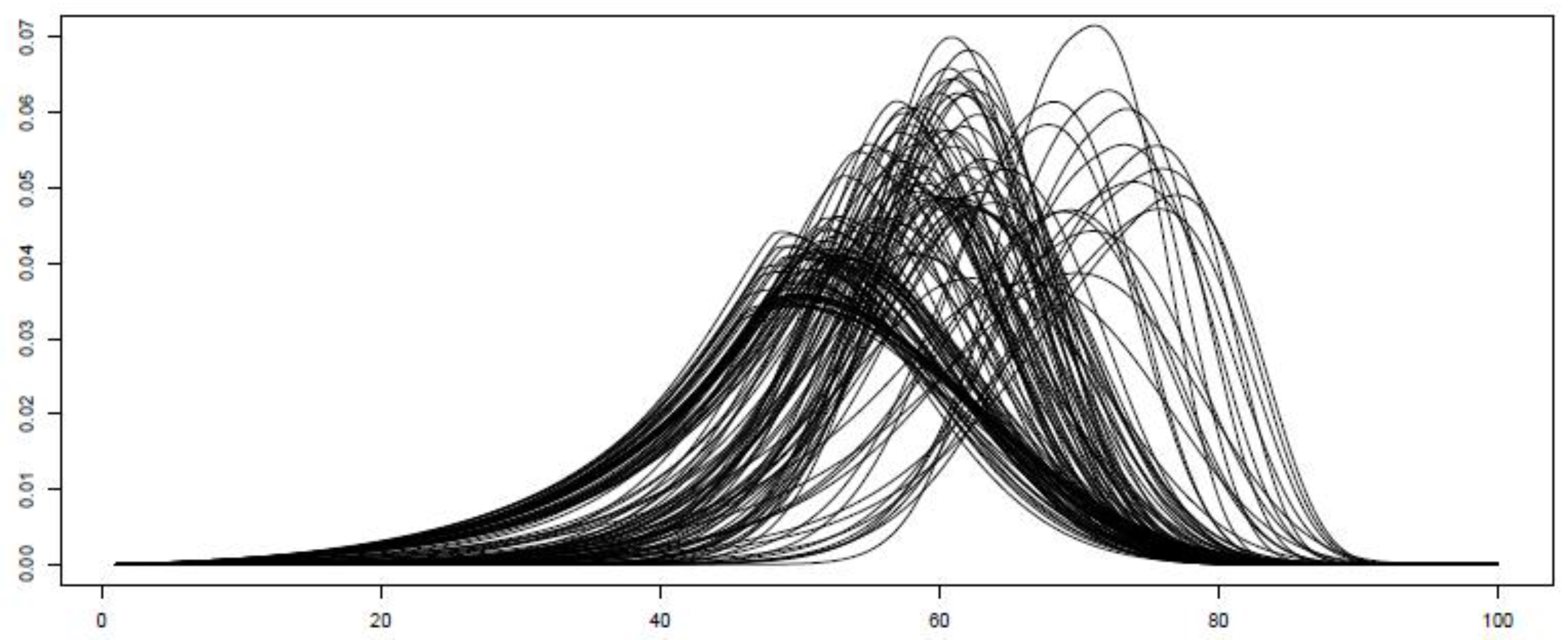
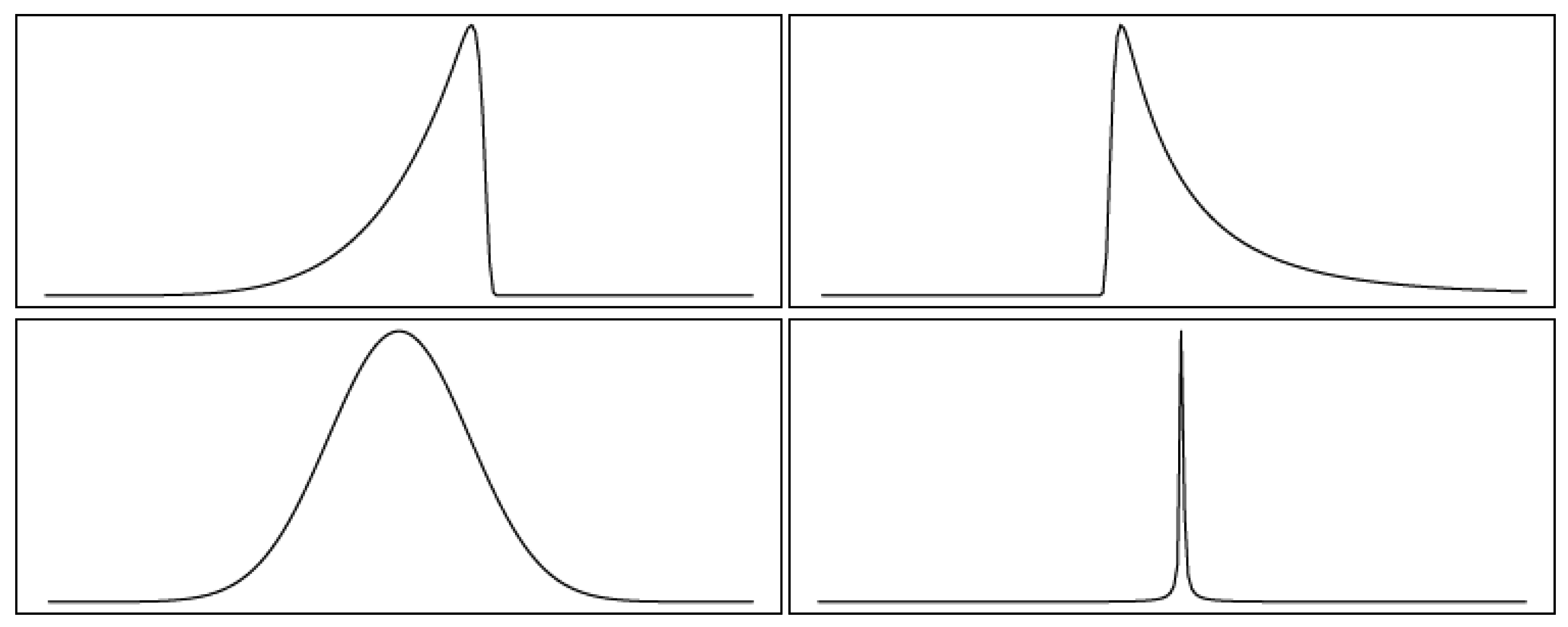
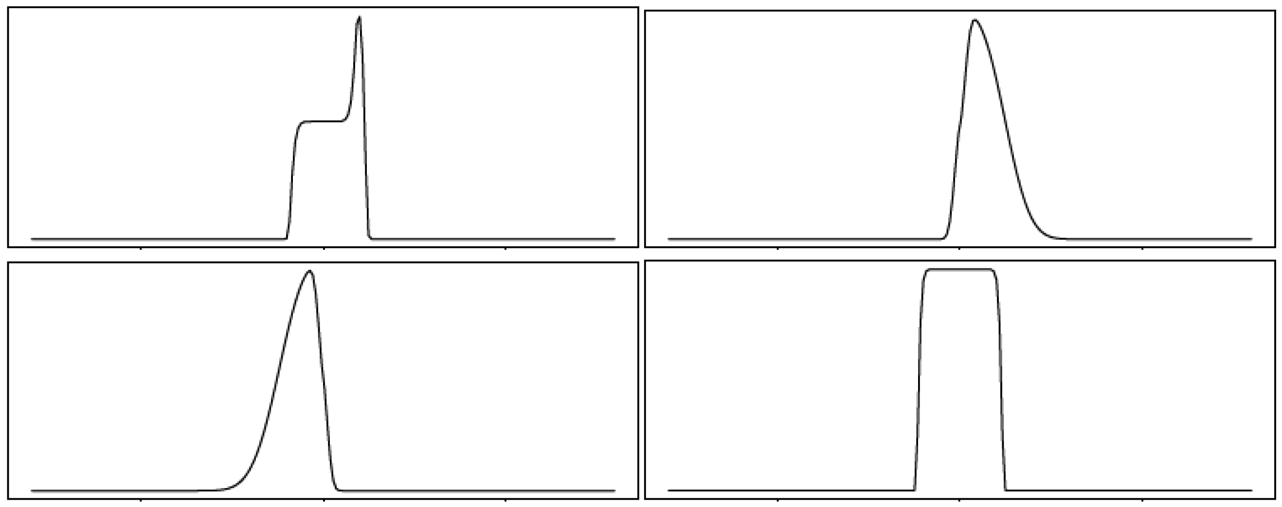
First, we illustrate the flexibility of these models in capturing a wide diversity of shapes of the probability density function (PDF). For example,
Figure 2 presents the predicted hourly PDF for the particular case of the BCPE model during one week of June 2014. As can be seen, this approach is able to encompass, among other characteristics, the features of asymmetry and fat tails.
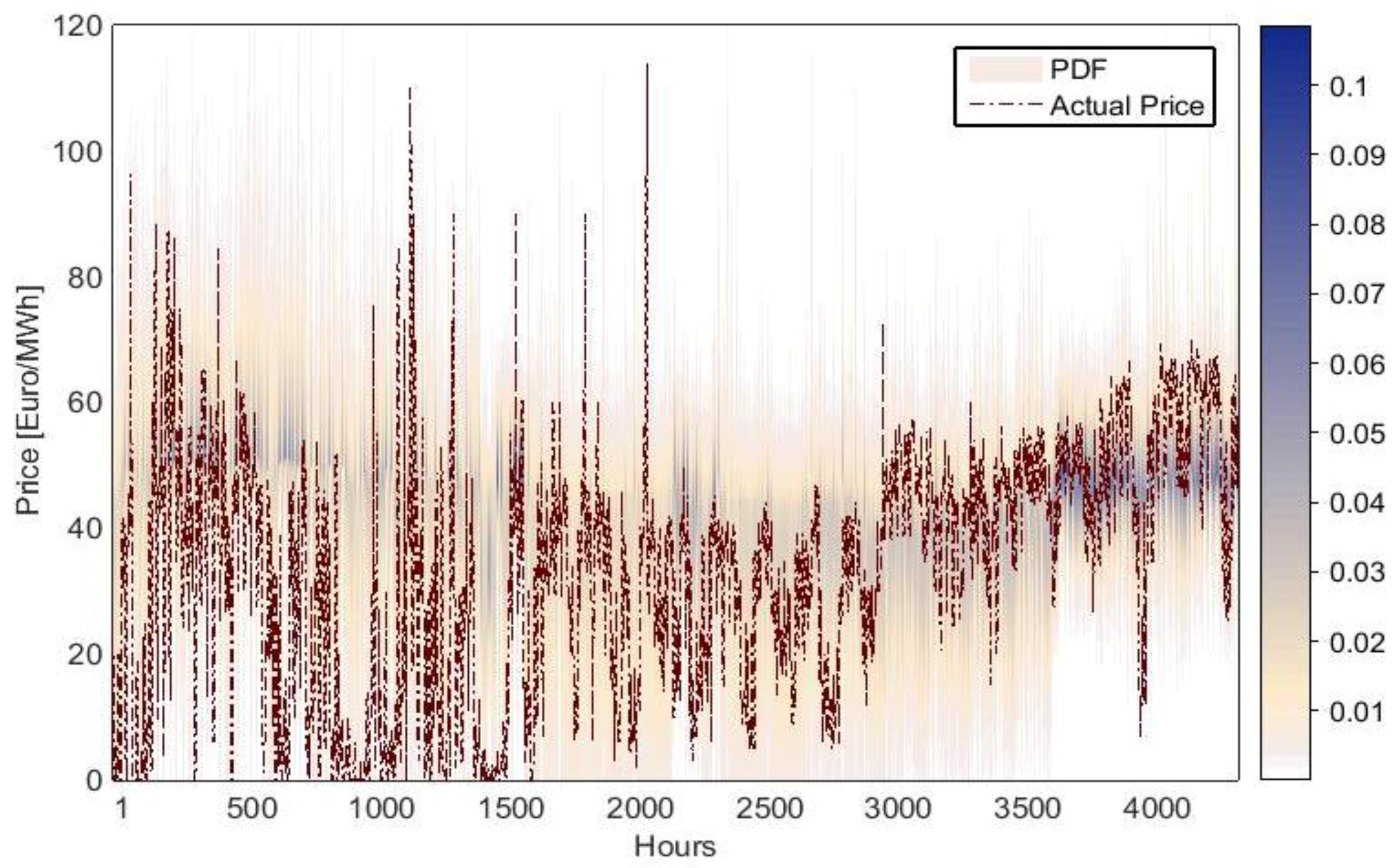
In addition to this,
Figure 3 shows the PDFs that have been estimated on an hourly basis with the SEP2 model. The color scale ranges from white (null probability) to blue (the highest predicted probability). It is evident that the actual price always falls within the range of predicted prices. Moreover, the actual price for most days is near the mode value, and the model assigns a high probability of occurrence to it.
Table 3 shows the exceedence rate for the seven target percentiles throughout the validation sample for each of the models. The proposed recalibration process is benchmarked against the uncalibrated market equilibrium model MEQ percentiles and the hybrid approach based upon recalibrations using conventional quantile regression (denoted as MEQ-QR), which performed best in [
4]. Overall, as seen in
Table 3, the proposed methodology is not outperformed by the nonparametric MEQ-QR benchmark, which furthermore does not offer analytical solutions, but would have been expected to estimate the percentiles more precisely. Moreover, the extreme quantiles appear to be better calibrated with the proposed parametric approach, which is crucial in risk analysis. This is consistent with the well-known underperformance of quantile regression in the extreme tails because of the scarcity of data points. Regarding the purely fundamental model (MEQ), it is evident that it does not fully capture all of the important characteristics of the electricity price series, particularly in the tails of the price density function where behavioral factors are apparently more relevant than basic fundamentals. Overall, these results validate the proposed parametric recalibration process as an effective methodology to capture not only the projected fundamental changes in the market, but also behavioral aspects.
3. Combinations for Increased Accuracy
In this section, we investigate if further modelling combinations can increase accuracy. We first observe that the MEQ-QR values could be taken as inputs to the GAMLSS recalibration process instead of the basic MEQ values. This approach has been indicated previously as the three-stage hybrid approach.
Table 4 reports a summary of the exceedance rates across the target quantiles. These findings demonstrate, perhaps not surprisingly, that the effectiveness of the hybrid recalibration technique is apparently increased if both quantile regression and GAMLSS recalibrations are used in sequence for additional refinement in model specification. Note that this three-stage hybridization scheme allows a relaxation of the constraints imposed to avoid the crossing between the quantile curves (since the most common approach to estimate quantile regression curves is to fit a function for each target percentile individually, the quantile curves can cross when multiple percentiles are estimated. This can lead to a lack of monotonicity and therefore, to an inconsistent distribution for the response) as these restrictions are naturally forced in the parametric distributions. Consequently, this fact leads to a major flexibility and a reduction in possible bias.
Also perhaps not surprising is that there is no clear winner amongst the different density models presented. It is appealing to observe that the three-stage approach with SEP2 distribution improves the forecasting accuracy in the center of the distribution, but loses precission at the tails in comparison to the two-stage approach. It is also of interest to note that a distribution such as ST3, that is not able to model platykurtosis in certain hours, gains accuracy in the upper tail of the distribution. This observation naturally leads to a proposal for combining the probabilistic forecasts.
It is well known for both point [
35] and density [
36,
37,
38] forecasting that combinations of forecasts may offer diversification gains and can provide insurance against possible model misspecification, data sets that are not sufficiently informative and structural changes (see [
39]). Although the idea of combining forecasts in itself is not new, it has been barely touched upon in the context of electricity spot prices (see the discussion of [
3]). Thus, we test different combination schemes on the methods (MEQ-QR-SEP2, MEQ-QR-SEP3 and MEQ-QR-ST3). Note that including MEQ-QR-BCPE, which is the worst model, in the combinations leads to poor forecasting performance. This is consistent, as expected, with [
40] and others who have observed that it is advisable to restrict combinations to a few good models.
Unlike [
41,
42], we used the probabilistic forecasts instead of the point predictions. As stated in [
35], combinations of probability density forecasts impose extra requirements beyond those that have been highlighted for combinations of point forecasts. The fundamental requirement is that the combination must be convex with weights restricted to the zero-one interval so that the probability forecast never becomes negative and always sums to one. Consistently with this prerequisite, we test equal weighting, as that is generally advocated as the most robust, and one performance-based weighting. For the latter, we use weights which are inversely proportional to the least absolute deviation (LAD).
The most natural approach to forecast averaging is the use of the arithmetic mean of all forecasts produced by the different models. This scheme, which is denoted as Equally Weighted Combination, EWC, is robust and is widely recommended in forecast combinations (see e.g., [
43,
44,
45]). In Equation (3) the EWC scheme is represented, where
is the number of methods used (three in the case study here presented: MEQ-QR-SEP2, MEQ-QR-SEP3, and MEQ-QR-ST3),
is the forecast of the price in hour
for the percentile
from parametric method
(i.e.,
, in which
is the unconditional CDF) and
is the final weighted prediction for the percentile
and hour
.
The other method for combining distributions we considered is based on the LAD, which hereinafter will be referred to as quantile regression averaging (QRA), and proceeds as follows:
- (1)
As in the previous combination approach, for each proposed parametric distribution function (MEQ-QR-SEP2, MEQ-QR-SEP3, and MEQ-QR-ST3), the corresponding quantile functions are derived for the usual target percentiles, so that . Note as the distribution functions vary with time (i.e., as the information set of explanatory variables evolves) so will the quantile functions.
- (2)
The predicted quantile functions
are combined for each percentile
using the asymmetric absolute loss function to yield the LAD regression. The LAD regression may be viewed as a particular case of quantile regression and intuitively, this method assigns specific weights for each percentile depending on the inverse of the absolute deviation error, so that larger weights are given to models that show smaller deviation error during the in-sample data set. Recall that the weights are sequentially updated after each additional moving window. As constructed quantile functions are sample unbiased, then we might expect that the weights’ sum to unity and there is strong intuitive appeal for omitting the constant (see [
46]).
Table 5 reports the accuracy metrics for the combinations. Again, there is not a clear winner in terms of forecasting performance. However, it seems that model averaging, following the discussion of [
47] and the findings of [
48] (in this reference, it is shown that simple combination schemes perform better than more sophisticated rules relying on estimating optimal weights that depend on the full variance-covariance matrix of forecast errors) and [
35] can capture different aspects of market conditions (particularly when the different approaches contain distinct information), provide a model diversification strategy that can improve forecasting robustness. As might be expected, this improvement is more apparent in the central percentiles than in the tails. Nevertheless, the improvements from these more elaborate combining methods are not huge and if the focus is upon tail risks it is better to find the best method instead of a combination. In these results, the indications are that ST3 is the most accurate for the high tails, and SEP3 for the low tails. All of this further vindicates the basic recalibration process based upon GAMLSS methodology.
4. Conclusions
The parametric recalibration methodology, as presented in this paper, offers a potentially valuable technique for the practical use of fundamental market models and their translation into well-calibrated density forecasts. The recalibration process improves accuracy compared to state of the art baseline techniques and is not substantially outperformed by more elaborate combining methods. Especially for the tail percentiles, where risk management is most crucial, the GAMLSS recalibration procedure—allied to the selection of an appropirate four parameter density function—would appear to offer the most accurate and analytically attractive approach to price density forecasting. In addition, the dynamic estimation of the first four moments is potentially beneficial in many analytical models of derivative pricing and portfolio optimization.
We did not discuss in detail the underlying fundamental model that was being recalibrated. In principle, the density recalibration process as presented, is applicacable to outputs from any fundamental model, whether such a model is a simple supply function stack or a computationally-intensive market equilibrium model. One would expect, however, that with simpler fundamental predictors, the scope for recalibration would be greater and that more exogenous variables would be significant in the dynamic estimation of the regressor coefficients for the latent moments. Nevertheless, selecting the appropriate regressors is a delicate process and overfitting should be a crucial concern in applying this methodology. Extensive out-of-sample validation testing is clearly required.


