Article

Improving the Stability and Accuracy of Power Hardware-in-the-Loop Simulation Using Virtual Impedance Method

1
School of Electrical Engineering, Wuhan University, Wuhan 430072, China
2
State Grid Henan Electric Power Research Institute, Zhengzhou 450000, China
*
Author to whom correspondence should be addressed.
Energies 2016, 9(11), 974; https://doi.org/10.3390/en9110974
Submission received: 13 September 2016 / Revised: 17 October 2016 / Accepted: 17 November 2016 / Published: 22 November 2016
(This article belongs to the Special Issue Next-Generation Low-Carbon Power and Energy Systems)

Abstract

:
Power hardware-in-the-loop (PHIL) systems are advanced, real-time platforms for combined software and hardware testing. Two paramount issues in PHIL simulations are the closed-loop stability and simulation accuracy. This paper presents a virtual impedance (VI) method for PHIL simulations that improves the simulation’s stability and accuracy. Through the establishment of an impedance model for a PHIL simulation circuit, which is composed of a voltage-source converter and a simple network, the stability and accuracy of the PHIL system are analyzed. Then, the proposed VI method is implemented in a digital real-time simulator and used to correct the combined impedance in the impedance model, achieving higher stability and accuracy of the results. The validity of the VI method is verified through the PHIL simulation of two typical PHIL examples.

1. Introduction

Power hardware-in-the-loop (PHIL) systems represent an emerging novel technique that is being increasingly applied in power systems for equipment testing and validation. The typical building blocks of a PHIL simulator are shown in Figure 1. Such a simulator is generally composed of three major parts: (I) the original power system (OPS), which is modeled in a real-time simulator; (II) the interface equipment (IE), which links the hardware and the simulated system [1]; and (III) the piece of hardware under test (HUT). The reference signal is obtained on the OPS side, and it is applied to the terminals of the actual hardware through the IE to establish a virtual exchange of power between the simulated virtual network and the power HUT. In a PHIL system, the simulated network and the HUT are both operating at a high power level [2,3,4,5]. Many simulation platforms that support PHIL simulations are commercially available [6,7,8,9,10,11,12,13,14], and such simulations have been extensively used for testing and design of distributed generation systems [15,16,17,18] and electric vehicles [19]. Moreover, PHIL systems offer several advantages over other analysis and testing methods. These systems minimize the cost and risk of examining various extreme conditions and maximize the likelihood of identifying hidden defects in an apparatus before their impacts are discovered in actual operations. Thus, the potentially serious consequences can be avoided.
The key element in a PHIL system is the simulation/hardware interface. Ideally, the IE between the HUT and the OPS should have an infinite bandwidth, unity gain, and zero time delay. However, an ideal IE in a PHIL system is neither achievable nor affordable. Moreover, some types of errors (IE bandwidth, sensor noise, time delay, and ripple of the IE) may cause severe stability issues or unacceptable accuracy issues in the results [20,21,22,23,24,25]. Therefore, these concerns are worth researching, both theoretically and practically. To address the stability issues of PHIL systems, various interface algorithms (IAs), which are used to connect the virtually simulated system and physical hardware, have already been proposed [26]. In the ideal transformer and inductor model (ITM) [27], the voltage amplifier reproduces the simulated voltage and imposes it onto the hardware circuit. The actual current is measured in the hardware circuit and fed back into the simulated circuit. An interface method that is based on a first-order approximation linear system has been proposed in [28]; it is based on the historical data collected, and the model coefficients are calculated and updated. However, this method is often ill-conditioned and yields incorrect coefficients [29]. Another approach, called the transmission-line model (TLM) [30], represents the linking of reactive components (i.e., inductors and capacitors) between the physical and simulated networks as a transmission line. However, the method does require the introduction of an interface series resistor on the physical side. This resistor is not part of the original network. Hence, the power loss in the resistor is not part of the system solution. The reference [31] described the five different interface algorithms, along with discussions of their relative strengths and weaknesses, with the damping impedance method (DIM) providing the better stability and accuracy. However, it is difficult to achieve the value of the damping impedance, especially in a complicated simulation. Meanwhile, other commonly employed methods, which include the addition of hardware and software filters, are described in [32,33], but, these methods heavily effect the accuracy of PHIL systems. Therefore, the search for a better method to improve the stability and accuracy of the PHIL simulations remains a research topic of considerable interest.
The impedance method has been widely used in grid-connected systems. The impedance of a grid-connected voltage-source converter is critical to any analysis of the stability and resonance between the converter and the grid, including that with the filter of the converter [34]. Particularly, a grid-connected voltage-source converter can be modeled as a current source in parallel with an impedance [35], and the stability of the system is determined by the magnitude of the impedance that can be improved by increasing the output impedance at the harmonic frequencies [36]. Similarly, to improve the stability of a PHIL system [37,38], a virtual impedance (VI) method [39,40,41] can be introduced.
This paper is the first to describe the application of the VI method to improve the stability and accuracy of the PHIL simulations. This method can be conveniently implemented on the OPS side. The stability criterion for a PHIL simulation is based on the equivalent impedance model, which is a simple model including an OPS impedance and a combined impedance of the HUT and the IE. The VI method is used to correct the combined impedance in the impedance model. The accuracy of a PHIL system has also been investigated and is herein discussed. Through the PHIL simulations of two typical PHIL examples, it is revealed that the VI method obtains a higher stability and accuracy than another method.
The remainder of this paper is organized as follows. In Section 2, the impedance model of the PHIL simulation is established. The stability and accuracy of the PHIL simulation are analyzed. Then, the VI method and its design rules are presented in Section 3. In Section 4, PHIL simulation results are reported to verify the effectiveness of the proposed method. Finally, Section 5 presents the conclusions.

2. Modeling of a PHIL System

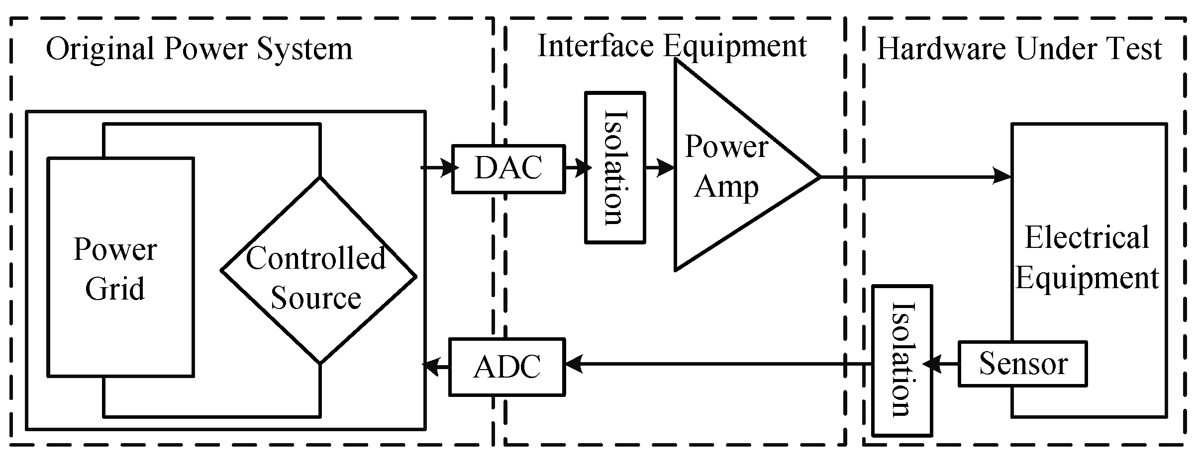
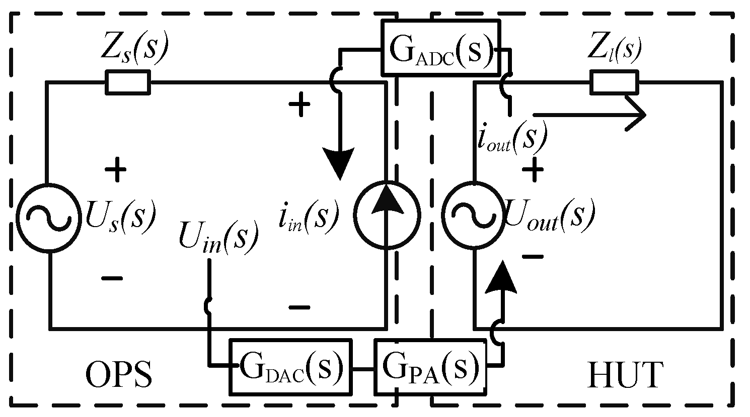
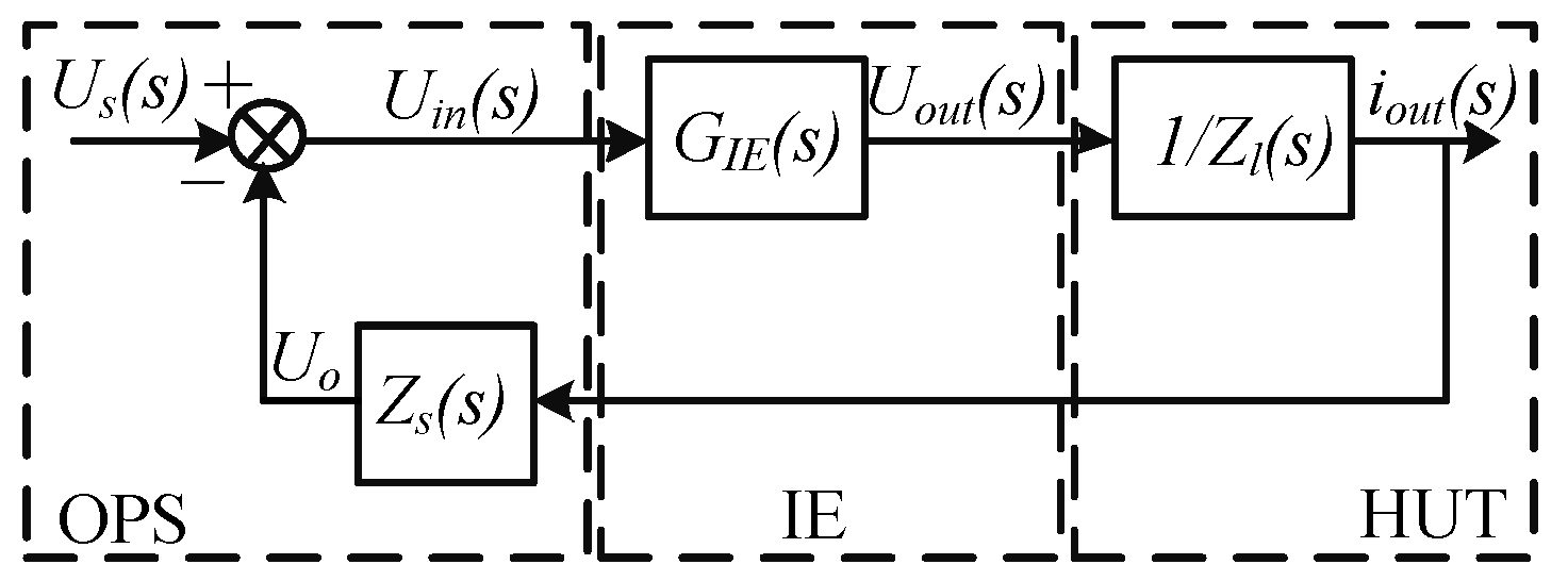
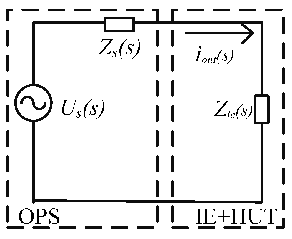
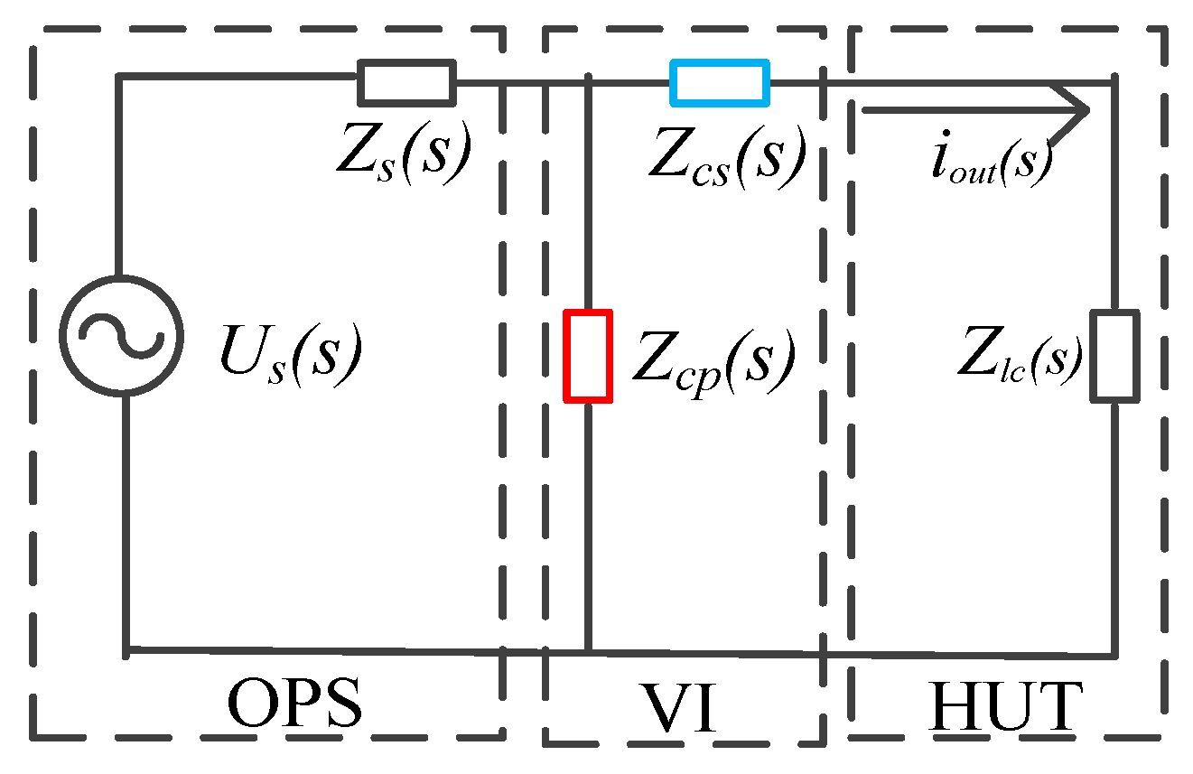
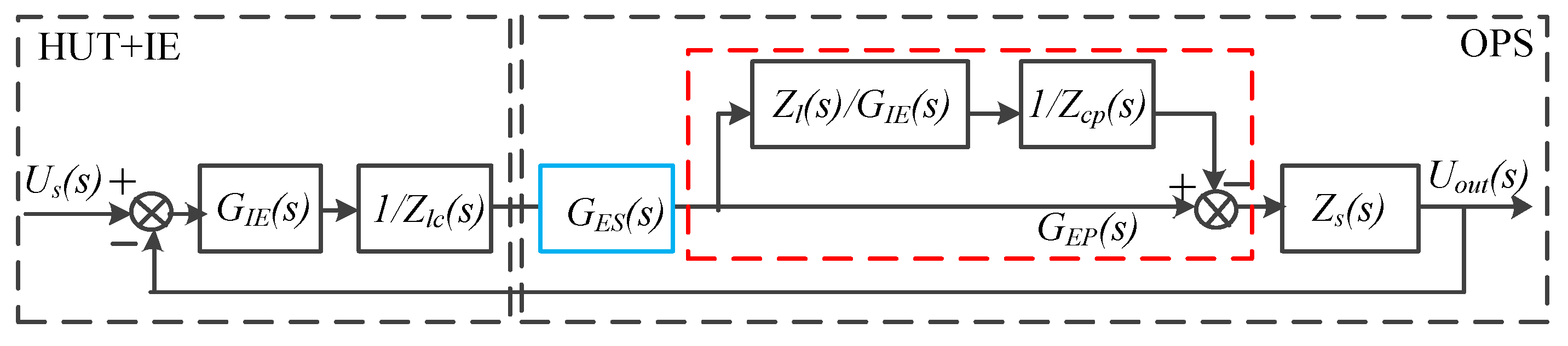
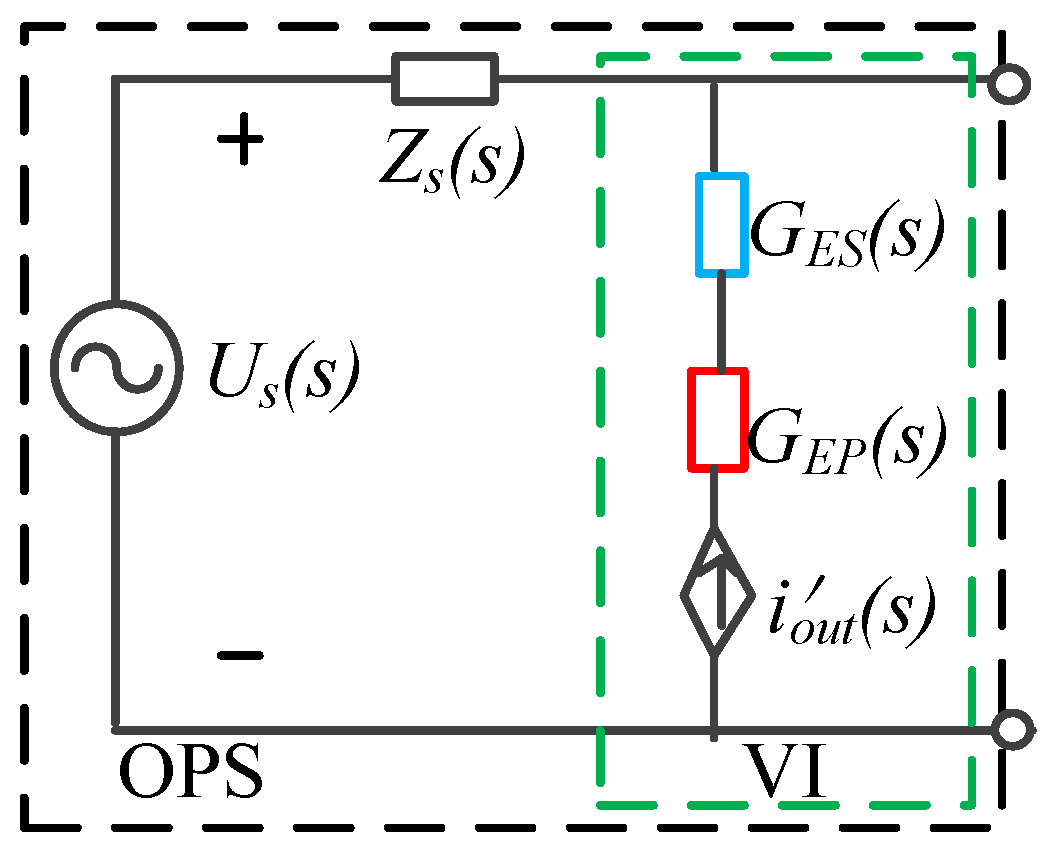
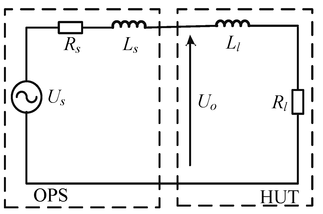
2.1. PHIL System Model

Figure 1 shows the overall architecture of a PHIL simulation. As mentioned in the introduction, the system consists of three fundamental subsystems: the original power system (OPS), the interface equipment (IE) and the hardware under test (HUT). As shown in Figure 1, the IE connects the real-time simulator and the real system. The most important components of the IE are the power amplifier (PA), a digital-to-analog converter (DAC) and an analog-to-digital converter (ADC).
The generic PHIL model, shown in Figure 2, is based on the ideal transformer method (ITM) [29]. The ITM is one of the most conventional and straightforward methods for implementing a PHIL simulation.
This paper focuses on the simulation of the power grid (OPS side). The majority of the grid impedance arises from long distribution wires and low-power transformers. This impedance can be modeled as an inductor in series with a resistor for simplicity. Therefore, this impedance can be modeled by its Thévenin equivalent. An ideal grid voltage source Us(s) is placed in series with a grid impedance Zs(s) on the OPS side. The load Zl(s) is the equivalent load on the HUT side. To facilitate the simulation, a voltage amplifier reproduces the simulated voltage Uin(s) as a physical voltage Uout(s) and imposes it on the load resistor. The actual current iout(s) drawn by the resistor is measured, and the measured signal is fed back into the simulated circuit by a current source producing a current iin(s). The main procedures for a PHIL simulation is described as follows.
To build an accurate and flexible PHIL system, a PA in the laboratory is applied. The schematic diagram of the PA, which employs a single-phase H-bridge converter connected to the HUT, is provided in Figure 3. An output filter is used to suppress high-frequency switching components to prevent them from entering the HUT.
As shown in Figure 4, a voltage controller Gc(s) based on the Proportion Integration (PI) controller is proposed. Gc(s) can be formulated as
G c ( s ) = K p + K i s .
To achieve a higher stability of the PA, an active damping factor Kc for the PA inverter is added to the system. The digital controller of the PA is subject to a computation delay, a pulse-width modulation (PWM) delay and other delay components, which can be represented by Gd(s). KPWM represents the transfer function of the inverter. Thus, the transfer function of the PA can be formulated as
G P A ( s ) = K p w m G d ( s ) G c ( s ) L C s 2 + K p w m K c G d ( s ) + K p w m G d ( s ) G c ( s ) .
DAC and ADC interface cards are needed to exchange signals between the real-time simulator and the hardware. For simplicity, the DAC and ADC are considered as part of an approximate equivalent model of the interface subsystem. The transfer function of the DAC and ADC components of the interface GDA(s) includes a small time delay Td, and it can be formulated as
G D A ( s ) = e T d s .
For mathematical analysis, a simpler and approximate equivalent circuit is adopted, where GIE(s) represents the combination of GDA(s) and GPA(s):
G I E ( s ) = G P A ( s ) G D A ( s ) .
Thus, the equivalent transfer function block diagram of the PHIL simulation model can be established as shown in Figure 5.
To establish an equivalent impedance model, the equivalent circuit is formulated as
U i n ( s ) = U s ( s ) Z s ( s ) i o u t ( s ) .
The reference signal Uin(s) can be amplified into output voltage Uout(s) through the IE. The output voltage Uout(s) imposes on the HUT, which is formulated as
U o u t ( s ) = U i n ( s ) G I E ( s ) .
According to Kirchhoff’s law, the following two equations can be obtained:
Z l ( s ) = U o u t ( s ) / i o u t ( s ) = U i n ( s ) G I E ( s ) / i o u t ( s ) ,
Z l c ( s ) = U i n ( s ) / i o u t ( s ) = Z l ( s ) / G I E ( s ) .
According to Equations (5)–(8), Zl(s) can be converted into a combined impedance Zlc(s) that includes GIE(s). Thus, the impedance model illustrated in Figure 6 is obtained. The stability and accuracy analysis based on this model are described as followings.

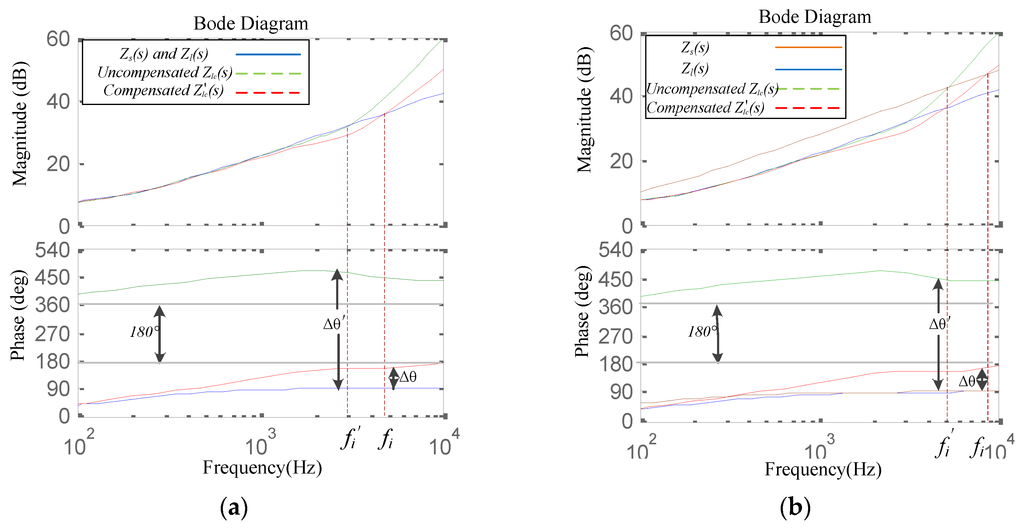
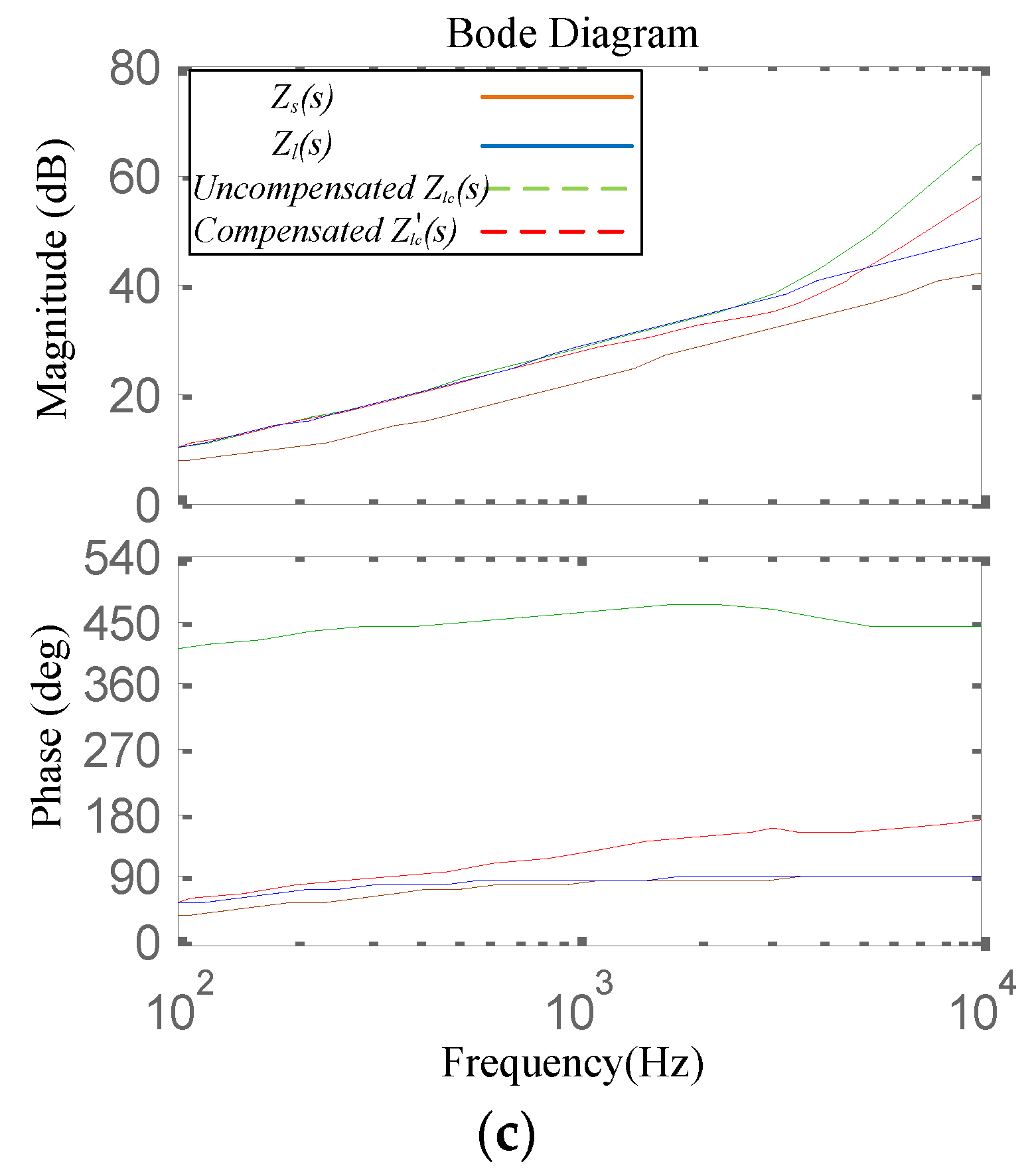
2.2. Stability Analysis

A PHIL simulation system can be represented by the equivalent circuit depicted in Figure 6, for which the output current can be written as
i o u t ( s ) = U s ( s ) Z s ( s ) + Z l c ( s ) .
This can be rearranged to yield the following equation:
i o u t ( s ) = U s ( s ) Z s ( s ) 1 1 + Z l c ( s ) / Z s ( s ) .
In this case, it is assumed that the source voltage is stable when the system is unloaded. Hence, both Us(s) and 1/Zs(s) are stable; therefore, the stability of the current depends on the stability of the second term on the right-hand side of Equation (10). The stability of the system can be estimated from the following equation:
H ( s ) = 1 1 + Z l c ( s ) / Z s ( s ) .
Therefore, Zlc(s) and Zs(s) determine the stability of the PHIL system. According to [42], if the frequency responses of Zs(s) and Zlc(s) intersect at fi, then the phase margin (PM) must be positive (PM > 0°). Thus, PM is formulated as
P M = 180 ° { arg [ Z s ( s ) ] arg [ Z l c ( s ) ] } .
To improve the stability of the system, it is necessary to compensate and correct for the combined impedance Zlc(s). To this end, the magnitude and phase margin of the combined impedance Zlc(s) are increased near the intersection frequency.

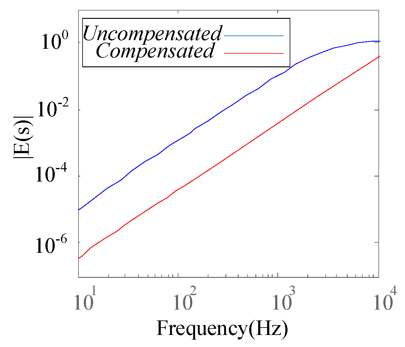
2.3. Accuracy Evaluation

The accuracy of a PHIL simulation can be estimated by comparing the combined impedance Zlc(s) to the actual impedance Zl(s). Because most of the errors in such a system arise from the IE, the impedance error is calculated based on the HUT subsystem, where the combined impedance Zlc(s) is the most important component in terms of accuracy. The impedance error E(s) can be evaluated as follows:
E ( s ) = | Z l ( s ) Z l c ( s ) Z l ( s ) | .

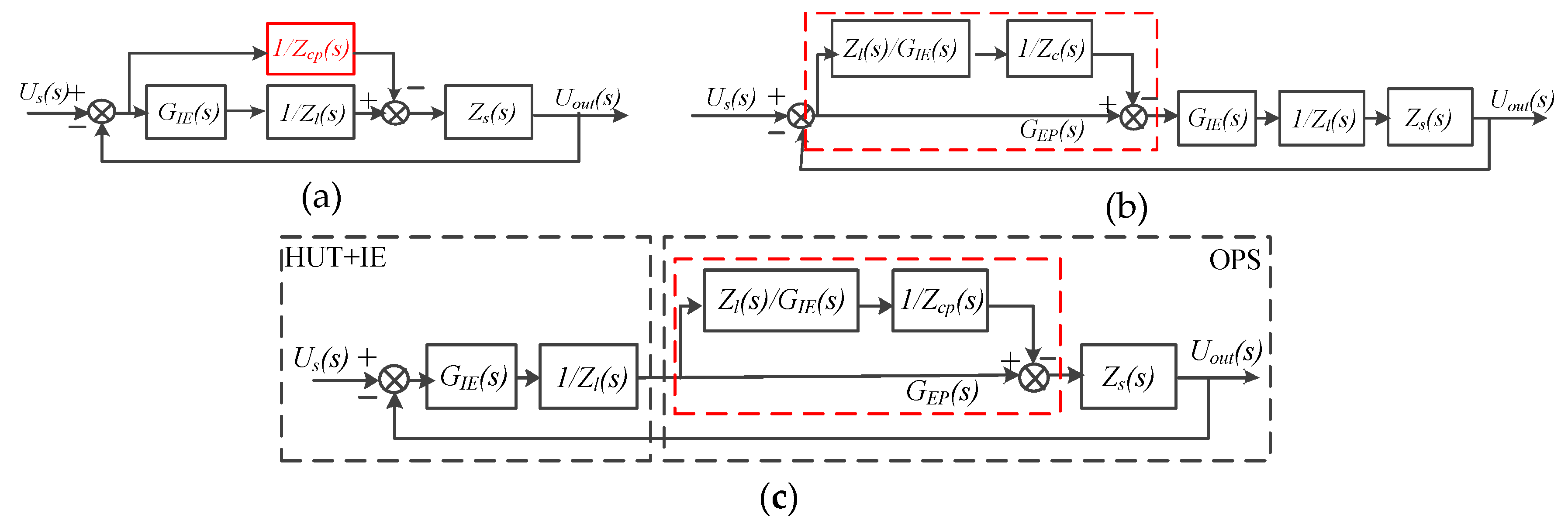
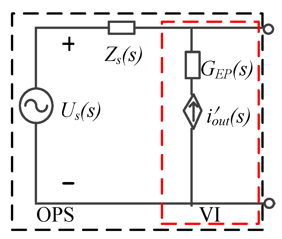
3. Proposal to Improve the Stability and Accuracy of PHIL Simulations

Based on the impedance model, the combined impedance Zlc(s) can be shaped by means of the VI. Thus, the accuracy of a PHIL simulation can be enhanced by introducing a paralleling impedance to shape the combined impedance Zlc(s).
Figure 7 shows the equivalent circuit for the PHIL simulation system with a paralleling impedance Zcp(s).
The shaped impedance Zeq(s) becomes
Z e q ( s ) = Z c p ( s ) Z l c ( s ) Z c p ( s ) + Z l c ( s ) = Z c p ( s ) Z l ( s ) / G I E ( s ) Z c p ( s ) + Z l ( s ) / G I E ( s ) .
As shown in Equation (14), to compensate the magnitude of impedance Zlc(s), it is necessary to make the impedance Zeq(s) equal to the impedance Zl(s). Thus, the impedance Zcp(s) can be derived as follows:
Z c p ( s ) = Z l ( s ) 1 G I E ( s ) .
In this way, the impedance error introduced by the IE can be eliminated.
Figure 8 shows the block structure of the equivalent transfer function of the PHIL system with equivalent impedance. The basic model depicted in Figure 8a can be transformed into the diagram shown in Figure 8b. The equivalent transformation presented in Figure 8c shows the equivalent model as it is implemented on the OPS side.
Figure 9 illustrates the implementation of the paralleling impedance. Moreover, because of the flexibility of the PHIL system provided by software simulation, various function blocks can be easily implemented in the simulation for a signal preprocessing. As shown in Figure 9, the introduction of the compensated block GEP(s) does not alter the PHIL system topology, it simply requires the insertion of a function block in the path of the feedback current signal to compensate for the error in the PHIL system. The equivalent transfer function can be calculated as follows:
G E P ( s ) = 1 G I E ( s ) = L C s 2 + K p w m K c G d ( s ) + K p w m G c ( s ) G d ( s ) K p w m G c ( s ) G d ( s ) .
The paralleling impedance improves the simulation performance of the PHIL system. However, the shaped impedance Zcp(s) may still intersect with impedance Zs(s) in the high-frequency range. Thus, an additional series virtual impedance is proposed. Figure 10 shows the structure of the PHIL system with the addition of a series impedance Zcs(s).
This series impedance is equivalent to a low-pass filter, the purpose of which is to ensure system stability and to avoid high-frequency components arising from numerical computations. The equivalent series impedance can be obtained as follows:
G E S ( s ) = 5000 s + 5000 .
The equivalent transformation is presented in Figure 11. The equivalent model is implemented on the OPS side.
Figure 12 illustrates the implementation of the series impedance. This function block can be easily implemented on the OPS side.

4. Experimental Verification

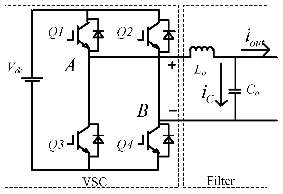
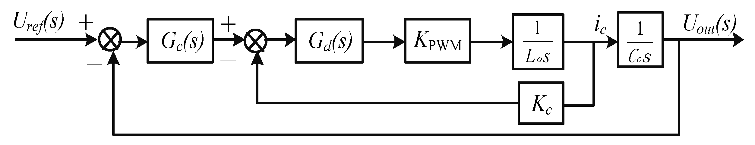
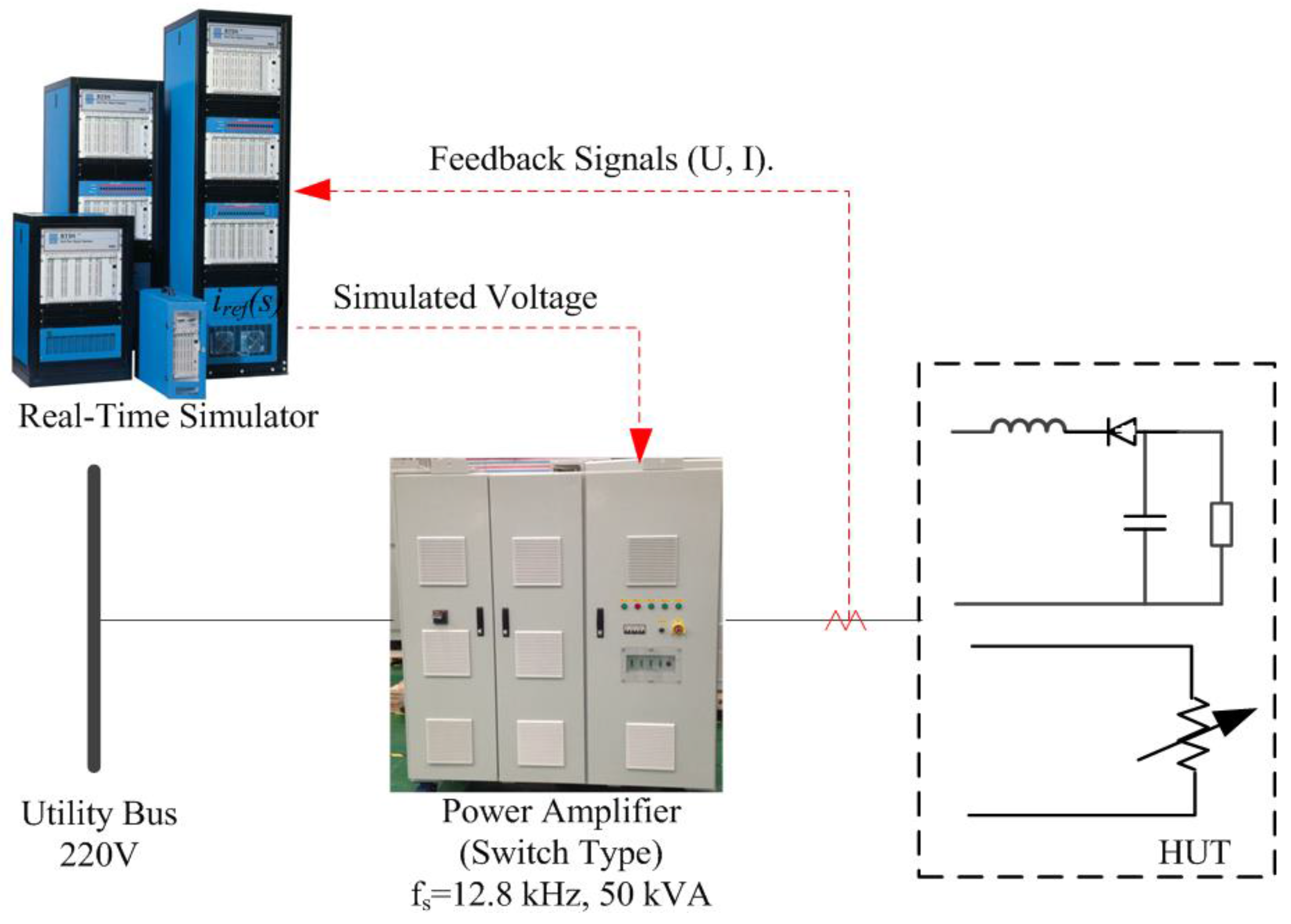
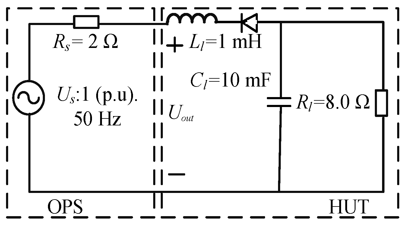
4.1. Description of the PHIL Platform

To verify the efficacy of the proposed method, two typical PHIL scenarios were simulated. Note that this paper focuses on the simulation of the power grid (OPS side). The majority of the grid impedance arises from long distribution wires and low-power transformers, and this impedance can be modeled as an inductor in series with a resistor for simplicity [42]. Firstly, a linear HUT scenario was theoretically analyzed. The impedance-based stability criterion was used to assess the stability of the PHIL system. The VI method was applied to this first scenario to improve the stability of the linear PHIL simulation. Then, a second scenario with a nonlinear HUT subsystem was established. A more complicated equivalent circuit was simulated to represent this scenario, and the validity of the VI method was again confirmed through this PHIL experiment.
Figure 13 shows the setup for the PHIL simulation platform. The platform included a real-time digital simulator (RTDS). The OPS was simulated in the RTDS using RTDS Technologies’ RSCAD graphical user interface (GUI) with a circuit simulation time step of 50 μs. An RTDS Giga-Transceiver Analogue Input (GTAI) card was used to import the feedback current signal. The reference output voltage signal was measured and transferred by a Giga-Transceiver Analogue Output (GTAO) card.
A prototype of a three-phase switch-type PA was built and tested in the lab. It includes three independent H-inverters and possesses the ability to generate PWM voltages from a constant direct current (DC)-voltage source. Field-programmable gate array (FPGA; EP4C115F23I7N) and advanced RISC (reduced instruction set computer) machine (ARM; STM32F417ZGT6) processors are used to control the PA. The switching frequency of the power amplifier is 12.8 kHz (with a sampling frequency of 25.6 kHz). The DC-link voltage is 450 V, and the output filter’s parameters are equal to Lo = 0.2 mH and Co = 60 μF. A PI controller is used as the output voltage regulator, with parameters of KP = 6 and Ki = 200, and the active damping regulator applies a damping factor of Kc = 5. A total time delay of 100 μs is assumed for the IE. For further analysis and comparison, the voltages are represented as per-unit (p.u.) values.
Stability Analysis: The original circuit for the first scenario was simulated using the PHIL model as shown in Figure 14. It can be assumed that impedance Zs is a combination of inductor Ls and resistor Rs and that impedance Zl is a combination of inductor Ll and resistor Rl. The effects of different values of inductor Ls and inductor Ll on the simulation stability were investigated. Table 1 shows the simulation parameters used in the analysis.
The grid impedance Zs(s) and the impedance Zl(s) are set using the simulation parameters, which are shown in Table 1. The combined impedance Zlc(s) and the compensated impedance Zlc(s) can be calculated using Equations (18) and (19):
Z l c ( s ) = Z l ( s ) / G I E ( s ) ,
Z l c ( s ) = Z l c ( s ) / G E S ( s ) G E P ( s ) .
The frequency responses of the grid impedance Zs(s), the impedance Zl(s), the combined impedance Zlc(s), and the compensated impedance Zlc(s) are shown in Figure 15.
Figure 15a,b show that the phase difference between impedance Zs(s) and the uncompensated impedance Zlc(s) approaches 180° when inductor Ls is greater than or equal to inductor Ll, indicating that the PM is negative (PM < 0°). Thus, the PHIL simulation is unstable. By contrast, when inductor Ls is smaller than inductor Ll, the simulation is stable. Figure 15c shows that in Case 3, there is no frequency intersection in the high-frequency range, as estimated using the impedance model. It is found that the compensated impedance Zlc(s) and impedance Zs(s) lead to critical stability. Thus, the stability of PHIL simulations can be improved using the VI method.
Accuracy Analysis: To describe the accuracy of the PHIL simulation without compensation, Equation (13) can be simplified to
E ( s ) = | Z l ( s ) Z l c ( s ) Z l ( s ) | = | 1 1 G I E ( s ) | .
The accuracy of the compensated PHIL system can be calculated as
E ( s ) = | Z l ( s ) Z l c ( s ) G E P ( s ) Z l ( s ) | = | 1 G E P ( s ) G I E ( s ) | .
The impedance error of the PHIL simulation is illustrated in Figure 16. The compensated error that is calculated using Equation (21) is less than the uncompensated error calculated using Equation (20).

4.2. Experimental Results

To confirm the efficacy of the proposed method, two typical PHIL simulations were established and tested. The proposed method was compared with the typical ITM method [29], which is one of the most conventional and straightforward methods of implementing PHIL simulations.

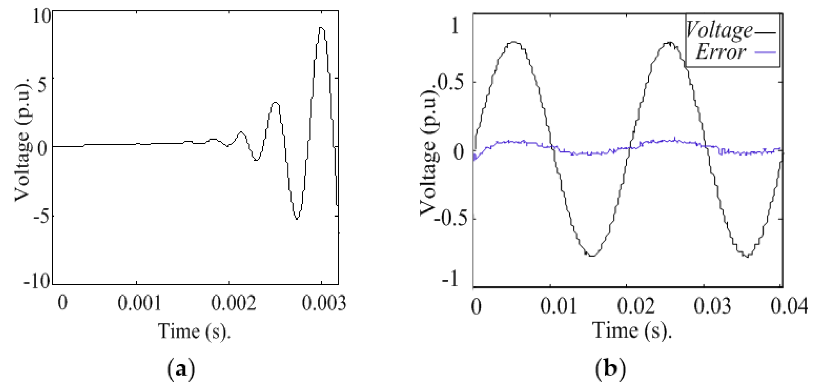
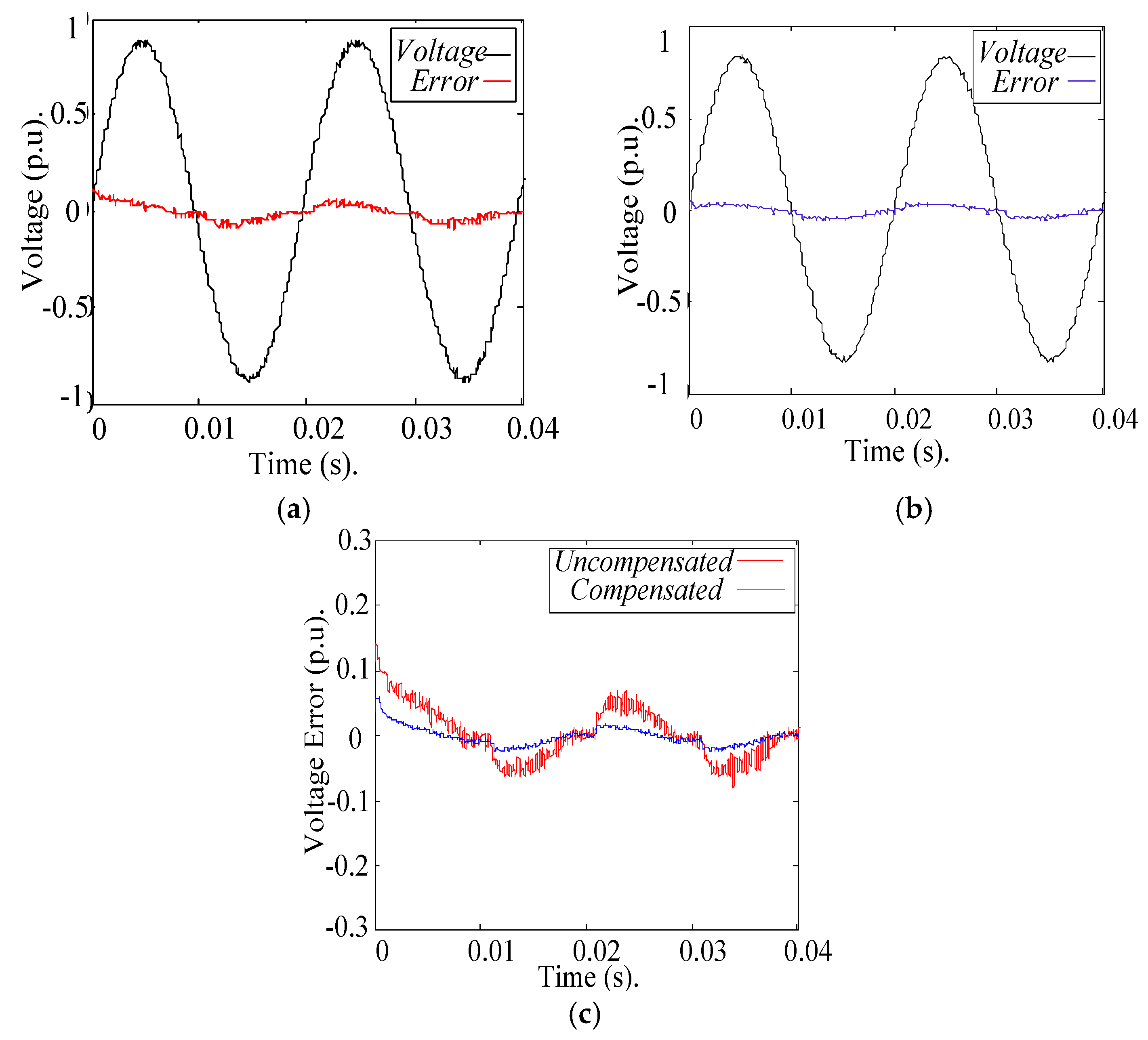
Scenario 1: Hardware with Linear Behavior 

As shown in Figure 14, the first considered scenario involved the resistor R and inductor L load circuit. The values of resistor R and inductor L are listed in Table 1. The simulation time step was set to 50 µs, and the parameters of the PA were designed as described in Section 4.1.
Simulations were operated with various values of inductor Ll and inductor Ls, and the output voltage waveforms and simulation errors for two cases are shown in Figure 17 and Figure 18. Figure 17a and Figure 18a show that the uncompensated PHIL simulation is unstable when inductor LsLl, whereas Figure 17b and Figure 18b show that the stability is significantly improved using the VI method.
Figure 19a,b show that when inductor Ls < Ll, the output voltage and the output voltage errors are improved, and Figure 19c shows that the accuracy is also improved. Thus, the effectiveness of the proposed method is confirmed.

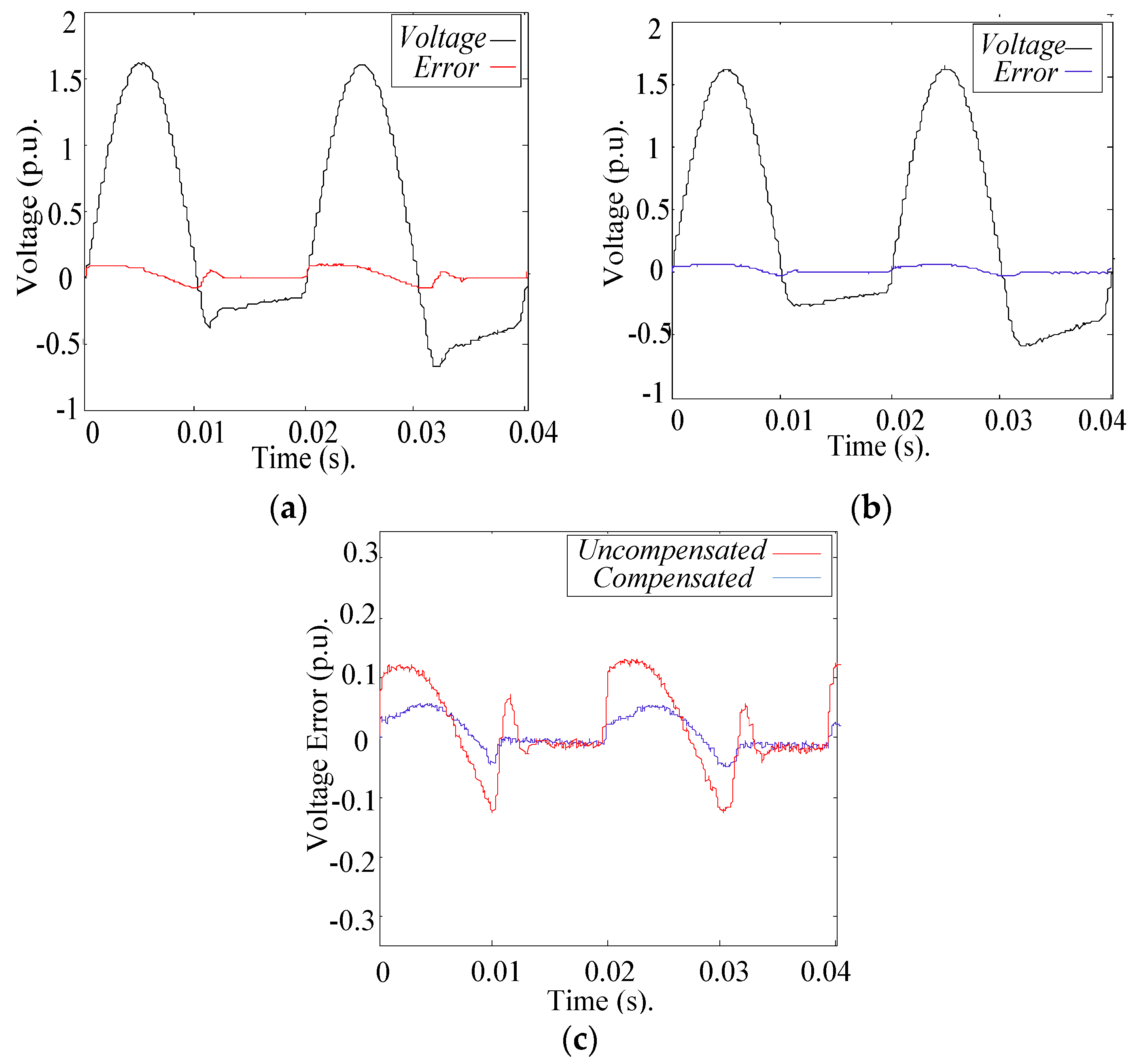
Scenario 2: Hardware with Nonlinear Behavior 

In practice, there are always nonlinear components on the HUT side. Thus, in the second considered PHIL scenario, a diode rectifier, which is a typical nonlinear device, is used. The circuit diagram is shown in Figure 20. In this case, the inductor is placed in series with a diode block, and a small capacitor is placed in parallel with the resistor. The parameters of the simulated circuit are shown in Figure 20. The simulation time step was set to 50 µs, and the parameters of the PA were designed as described in Section 4.1.
Figure 21 compares the experimental results for the uncompensated and compensated PHIL simulations. Better accuracy is achieved in the compensated PHIL simulation, confirming the effectiveness of the proposed compensation method.

5. Conclusions

This paper presents an effective VI method for enhancing the stability and accuracy of PHIL simulations. The proposed VI method is easy to be implemented in a digital real-time simulator. The VI method offers greatly simplified implementation on the OPS side. Therefore, it is suitable for most practical PHIL simulations involving highly complex circuits and nonlinear components. Through the establishment of an impedance model for a PHIL simulation, the stability and accuracy of the system can be analyzed. Furthermore, the stability and accuracy of PHIL simulations can be improved using the VI method. Simulations of two typical PHIL cases (one linear HUT and one nonlinear HUT) are presented to demonstrate these improvements, thereby verifying the validity of the VI method.

Acknowledgments

Project sponsored by the National key research and development program of China (2016YFB0900404).

Author Contributions

Xiaoming Zha, Chenxu Yin and Jianjun Sun designed the main components of the study, including the PHIL model, the VI method, the analyses of the stability and accuracy, the PHIL platform setup. Chenxu Yin is responsible for writing the paper. Meng Huang and Qionglin Li mainly worked on the dynamic analyses of the simulated data.

Conflicts of Interest

The authors declare no conflicts of interest.

References

  1. Ren, W.; Sloderbeck, M.; Steurer, M.; Dinavahi, V.; Noda, T.; Filizadeh, S.; Chevrefils, A.R.; Matar, M.; Iravani, R.; Dufour, C.; et al. Interfacing issues in real-time digital simulators. IEEE Trans. Power Deliv. 2011, 26, 1221–1230. [Google Scholar] [CrossRef]
  2. Steurer, M.; Edrington, C.S.; Sloderbeck, M.; Ren, W.; Langston, J. A megawatt-scale power hardware-in-the-loop simulation setup for motor drives. IEEE Trans. Ind. Electron. 2010, 57, 1254–1260. [Google Scholar] [CrossRef]
  3. Li, H.; Steurer, M.; Shi, K.L.; Woodruff, S.; Zhang, D. Development of a unified design, test, and research platform for wind energy systems based on hardware-in-the-loop real-time simulation. IEEE Trans. Ind. Electron. 2006, 53, 1144–1151. [Google Scholar] [CrossRef]
  4. Liu, Y.; Steurer, M.; Ribeiro, P. A novel approach to power quality assessment: Real time hardware-in-the-loop test bed. IEEE Trans. Power Deliv. 2005, 20, 1200–1201. [Google Scholar] [CrossRef]
  5. Tucker, J. Power-Hardware-In-the-Loop (PHIL) Considerations and Implementation Methods for Electrically Coupled Systems. Master’s Thesis, University of South Carolina, Columbia, SC, USA, 2011. [Google Scholar]
  6. Etemadi, A.H.; Iravani, R. Overcurrent and overload protection of directly voltage-controlled distributed resources in a microgrid. IEEE Trans. Ind. Electron. 2013, 60, 5629–5638. [Google Scholar] [CrossRef]
  7. Li, H.; Guo, F.; Yang, S.; Zhu, L.; Yao, C.; Wang, J. Usage profile optimization of the retired PHEV battery in residential microgrid. In Proceedings of the IEEE Transportation Electrification Conference and Expo, Asia-Pacific, Beijing, China, 31 August–3 September 2014; pp. 1–6.
  8. Guo, F.; Herrera, L.; Alsolami, M.; Li, H.; Xu, P.; Lu, X.; Lang, A.; Wang, J.; Long, Z. Design and development of a reconfigurable hybrid Microgrid test bed. In Proceedings of the IEEE Energy Conversion Congress and Exposition (ECCE), Denver, CO, USA, 15–19 Septemer 2013; pp. 1350–1356.
  9. Hwang, T.; Park, S. A seamless control strategy of a distributed generation inverter for the critical load safety under strict grid disturbances. IEEE Trans. Power Electron. 2013, 28, 4780–4790. [Google Scholar] [CrossRef]
  10. Dufour, C.; Bélanger, J. On the use of real-time simulation technology in smart grid research and development. IEEE Trans. Ind. Appl. 2014, 50, 3963–3970. [Google Scholar] [CrossRef]
  11. Ivanović, Z.R.; Adžić, E.M.; Vekić, M.S.; Grabić, S.U.; Čelanović, N.L.; Katić, V.A. HIL evaluation of power flow control strategies for energy storage connected to smart grid under unbalanced conditions. IEEE Trans. Power Electron. 2012, 27, 4699–4710. [Google Scholar] [CrossRef]
  12. Park, M.; Yu, I. A novel real-time simulation technique of photovoltaic generation systems using RTDS. IEEE Trans. Energy Convers. 2004, 19, 164–169. [Google Scholar] [CrossRef]
  13. Adzic, E.; Grabic, S.; Vekic, M.; Porobic, V.; Celanovic, N.F. Hardware-in-the-loop optimization of the 3-phase grid connected converter controller. In Proceedings of the 39th Annual Conference of the IEEE Industrial Electronics Society, Vienna, Austria, 10–13 November 2013; pp. 5392–5397.
  14. Knauff, M.; Schegan, C.; Chunko, J.; Fischl, R.; Miu, K. A preliminary modeling and simulation platform to investigate new shipboard power system prototyping techniques. In Proceedings of the Grand Challenges in Modeling and Simulation, Istabul, Turkey, 13–16 July 2009; pp. 198–204.
  15. Oh, S.; Yoo, C.; Chung, I.; Won, D. Hardware-in-the-loop simulation of distributed intelligent energy management system for Microgrids. Energies 2013, 6, 3263–3283. [Google Scholar] [CrossRef]
  16. Shiau, J.; Lee, M.; Wei, Y.; Chen, B. Circuit simulation for solar Power maximum Power Point tracking with different Buck-Boost converter topologies. Energies 2014, 7, 5027–5046. [Google Scholar] [CrossRef]
  17. Calise, F.; Capuano, D.; Vanoli, L. Dynamic simulation and Exergo-Economic optimization of a hybrid solar–geothermal cogeneration plant. Energies 2015, 8, 2606–2646. [Google Scholar] [CrossRef]
  18. Marco, J.; Kumari, N.; Widanage, W.D.; Jones, P. A cell-in-the-loop approach to systems modelling and simulation of energy storage systems. Energies 2015, 8, 8244–8262. [Google Scholar] [CrossRef]
  19. Locment, F.; Sechilariu, M. Modeling and simulation of DC Microgrids for electric vehicle charging stations. Energies 2015, 8, 4335–4356. [Google Scholar] [CrossRef]
  20. Lehfuss, F.; Lauss, G.; Kostampopoulos, P.; Hatziargyriou, N.; Crolla, P.; Roscoe, A. Comparison of multiple power amplification types for power hardware-in-the-loop applications. In Proceedings of the IEEE Workshop Complexity Engineering, Aachen, Germany, 11–13 June 2012; pp. 1–6.
  21. Lauss, G.; Faruque, M.O.; Schoder, K.; Dufour, C.; Viehweider, A.; Langston, J. Characteristics and design of Power hardware-in-the-loop simulations for electrical Power systems. IEEE Trans. Ind. Electron. 2016, 63, 406–417. [Google Scholar] [CrossRef]
  22. Viehweider, A.; Lauss, G.; Lehfuss, F. Interface and stability issues for SISO and MIMO power hardware in the loop simulation of distribution networks with photovoltaic generation. Int. J. Renew. Energy Res. 2012, 2, 632–639. [Google Scholar]
  23. Wu, X.; Lentijo, S.; Deshmuk, A.; Monti, A.; Ponci, F. Design and implementation of a power-hardware-in-the-loop interface: A nonlinear load case study. In Proceedings of the Twentieth Annual IEEE Applied Power Electronics Conference and Exposition, Urbana, IL, USA, 6–10 March 2005.
  24. Ayasun, S.; Fischl, R.; Chmielewski, T.; Vallieu, S.; Miu, K.; Nwankpa, C. Evaluation of static performance of simulation-stimulation interface for Power hardware in the loop. In Proceedings of the IEEE Power Tech Conference, Bologna, Italy, 23–26 June 2003.
  25. Jha, K.; Mishra, S.; Joshi, A. Boost-amplifier-based Power-hardware-in-the-loop simulator. IEEE Trans. Ind. Electron. 2015, 62, 7479–7488. [Google Scholar] [CrossRef]
  26. Lentijo, S.; D’Arco, S.; Monti, A. Comparing the dynamic performances of power hardware-in-the-loop interfaces. IEEE Trans. Ind. Electron. 2010, 57, 1195–1207. [Google Scholar] [CrossRef]
  27. Gan, C.; Todd, R.; Apsley, J.M. Drive system dynamics compensator for a mechanical system emulator. IEEE Trans. Ind. Electron. 2015, 62, 70–78. [Google Scholar] [CrossRef]
  28. Wu, X.; Lentijo, S.; Monti, A. A novel interface for power hardware-in-the-loop simulation. In Proceedings of the IEEE Workshop on Computers in Power Electronics (COMPEL 2004), Urbana, IL, USA, 15–18 August 2004; pp. 178–182.
  29. Ren, W.; Steurer, M.; Baldwin, T.L. Improve the stability and the accuracy of power hardware-in-the-loop simulation by selecting appropriate interface algorithms. IEEE Trans. Ind. Appl. 2008, 44, 1286–1294. [Google Scholar] [CrossRef]
  30. Feng, X.; Liu, J.; Lee, F.C. Impedance specifications for stable dc distributed power systems. IEEE Trans. Power Electron. 2002, 17, 157–162. [Google Scholar] [CrossRef]
  31. Paran, S.; Edrington, C.S. Improved power hardware in the loop interface methods via impedance matching. In Proceedings of the IEEE Electric Ship Technologies Symposium, Arlington, VA, USA, 22–24 April 2013; pp. 342–346.
  32. Siegers, J.; Santi, E. Improved power hardware-in-the-loop interface algorithm using wideband system identification. In Proceedings of the IEEE Applied Power Electronics Conference and Exposition, Fort Worth, TX, USA, 16–20 March 2014; pp. 1198–1204.
  33. Viehweider, A.; Lauss, G.; Felix, L. Stabilization of power hardware-in-the-loop simulations of electric energy systems. Simul. Model. Pract. Theory 2011, 19, 1699–1708. [Google Scholar] [CrossRef]
  34. Sun, J. Impedance-based stability criterion for grid-connected inverters. IEEE Trans. Power Electron. 2011, 26, 3075–3078. [Google Scholar] [CrossRef]
  35. He, J.; Li, Y.W.; Bosnjak, D.; Harris, B. Investigation and active damping of multiple resonances in a parallel-inverter-based microgrid. IEEE Trans. Power Electron. 2013, 28, 234–246. [Google Scholar] [CrossRef]
  36. Zhang, S.; Jiang, S.; Lu, X.; Ge, B.; Peng, F.Z. Resonance issues and damping techniques for grid-connected inverters with long transmission cable. IEEE Trans. Power Electron. 2014, 29, 110–120. [Google Scholar] [CrossRef]
  37. Wang, F.; Duarte, J.L.; Hendrix, M.A.M.; Ribeiro, P.F. Modeling and analysis of grid harmonic distortion impact of aggregated DG inverters. IEEE Trans. Power Electron. 2011, 26, 786–797. [Google Scholar] [CrossRef]
  38. Jia, Y.; Zhao, J.; Fu, X. Direct grid current control of LCL-filtered grid-connected inverter mitigating grid voltage disturbance. IEEE Trans. Power Electron. 2014, 29, 1532–1541. [Google Scholar]
  39. Lauss, G.; Lehfuss, F.; Viehweider, A.; Strasser, T. Power hardware in the loop simulation with feedback current filtering for electric systems. In Proceedings of the 37th Annual Conference on IEEE Industrial Electronics Society, Melbourne, Australia, 7–10 November 2011; pp. 3725–3730.
  40. Cespedes, M.; Sun, J. Impedance modeling and analysis of grid-connected voltage-source converters. IEEE Trans. Power Electron. 2014, 29, 1254–1261. [Google Scholar] [CrossRef]
  41. Ren, W.; Steurer, M.; Baldwin, T.L. An effective method for evaluating the accuracy of power hardware-in-the-loop simulations. IEEE Trans. Ind. Appl. 2009, 45, 1484–1490. [Google Scholar] [CrossRef]
  42. Yang, D.; Ruan, X.; Wu, H. Impedance shaping of the grid-connected inverter with LCL filter to improve its adaptability to the weak grid condition. IEEE Trans. Power Electron. 2014, 29, 5795–5806. [Google Scholar] [CrossRef]
Figure 1. Basic building blocks of a power hardware-in-the-loop (PHIL) simulation.
Energies 09 00974 g001
Figure 2. Structure diagram of a PHIL simulation system.
Energies 09 00974 g002
Figure 3. Switching power amplifier (PA) circuit.
Energies 09 00974 g003
Figure 4. Transfer function block diagram of the switching PA.
Energies 09 00974 g004
Figure 5. Transfer function block diagram of the PHIL simulation system.
Energies 09 00974 g005
Figure 6. Equivalent circuit for the PHIL simulation system.
Energies 09 00974 g006
Figure 7. Equivalent circuit for the PHIL simulation system with a paralleling virtual impedance (VI).
Energies 09 00974 g007
Figure 8. Transfer function diagram of the PHIL system: (a) s-domain model; (b) equivalent transformation I; (c) equivalent transformation II.
Energies 09 00974 g008
Figure 9. Implementation of a paralleling VI on the original power system (OPS) side.
Energies 09 00974 g009
Figure 10. Equivalent circuit for the PHIL system based on the VI model.
Energies 09 00974 g010
Figure 11. Transfer function block diagram for the PHIL system based on the VI model.
Energies 09 00974 g011
Figure 12. Implementation of the VI on the OPS side.
Energies 09 00974 g012
Figure 13. PHIL experimental setup.
Energies 09 00974 g013
Figure 14. Topology used in the first PHIL simulation scenario, with a linear resistance/inductor (RL) load circuit.
Energies 09 00974 g014
Figure 15. Frequency responses of different impedances Zs(s) and Zl(s), the combined impedance Zlc(s), and the compensated impedance Zlc(s): (a) Case 1; (b) Case 2; and (c) Case 3.
Energies 09 00974 g015aEnergies 09 00974 g015b
Figure 16. Diagram for evaluating the impedance accuracy of a PHIL simulation.
Energies 09 00974 g016
Figure 17. Scenario 1 simulation with Ls = 2 mH, Rs = 2 Ω, Ll = 2 mH, and Rl = 2 Ω: (a) uncompensated output voltage waveform and (b) compensated output voltage waveform.
Energies 09 00974 g017
Figure 18. Scenario 1 simulation with Ls = 4 mH, Rs = 2 Ω, Ll = 2 mH, and Rl = 2 Ω: (a) uncompensated output voltage waveform; (b) compensated output voltage waveform.
Energies 09 00974 g018
Figure 19. Scenario 1 simulation with Ls = 2 mH, Rs = 2 Ω, Ll = 4 mH, and Rl = 2 Ω: (a) uncompensated output voltage and error waveforms; (b) compensated output voltage and error waveforms; (c) magnified view of output voltage error waveforms.
Energies 09 00974 g019
Figure 20. Topology used in the second PHIL simulation scenario, with a nonlinear load.
Energies 09 00974 g020
Figure 21. Scenario 2 simulation with Rs = 2Ω, Ll = 1 mH, Cl = 10 mF, and Rl = 8 Ω: (a) uncompensated output voltage and error waveforms; (b) compensated output voltage and error waveforms; and (c) view of output voltage error waveforms.
Energies 09 00974 g021
Table 1. the value of the impedance Zs and impedance Zl.
ParameterValueParameterValue
Rs2 ΩRl2 Ω
LsCase (1): 2 mHLlCase (1): 2 mH
Case (2): 4 mHCase (2): 2 mH
Case (3): 2 mHCase (3): 4 mH

