Dynamic Simulation of a Trigeneration Scheme for Domestic Purposes Based on Hybrid Techniques

Abstract

In this paper, the design of a system providing electricity by coupling photovoltaic/thermal (PVT) collectors and a wind turbine (WT), sanitary hot water (SHW) coming from the PVT and evacuated tube collectors (ETCs) and fresh water (FW) produced in two seawater desalting facilities (membrane distillation, MD, and reverse osmosis, RO), has been carefully analyzed by means of a dynamic model developed in TRNSYS^®. This analysis is compulsory to operate a lab-scale pilot plant that is being erected at Zaragoza, Spain. A new model-type has been included in TRNSYS^® in order to include the MD unit in the scheme. A sensitivity analysis of some free-design variables, such that the ETC surface, PVT and ETC tilt, water storage tank, batteries capacities, and mass flow rates delivered to the SHW service and/or feeding the MD unit has been performed in order to propose the definite design of the scheme. The proposed base case was able to produce up to 15,311 L per year in the MD system and cover an electric energy demand of 1890 kWh. Coverage of SHW, water (including RO and MD) and power is respectively 99.3%, 100% and 70%. However, daily and yearly assessment of FW, SHW and power produced with the optimized design gave a better coverage of water and energy demands for a typical single family home. The improved and definite design was able to increase its MD production in 35% and the electric energy in 7% compared with base case.

1. Introduction

The need of safe-clean energy and water, especially in isolated areas in which power and water networks incur extra economic and environmental costs, is one of the challenges of the 21st century. The search for innovative and sustainable solutions to provide secure energy and water in isolated areas by integrating existing technologies is a reliable solution that should be explored. This paper is one attempt to solve this problem, providing a preliminary design for further implementation.

Nowadays, most of the energy produced around the world is obtained by burning fossil fuels. These kinds of fuels contribute to local air pollution, a significant decrease of woodlands around the world, ozone layer problems and higher temperatures around the whole planet [1]. For that reason, it is important to use alternative energy resources like solar and wind energy which could be sustainable options when mainly thermal and electric energy are required to produce sanitary hot water (SHW) or even fresh water (FW) [2].

In Europe, the solar thermal capacity is expected to reach about 150 to 250 GW by the year 2030, which would equate to a 7%–11% share of global electricity production [3]. With solar energy, both electricity and thermal energy can be obtained through the use of a photovoltaic/thermal (PVT) collector [4]. This hybrid collector integrates features of single photovoltaic and solar thermal systems in one combined product. The hybrid system basically consists of one absorbing plate to remove waste heat (cell cooling) from a photovoltaic panel (PV) through the circulation of a heat transfer fluid behind the PV cells [5]. This hybrid arrangement reduces the overall temperature losses on the collector and increases the global efficiency. In other words, the solar energy that is not transformed into electricity is converted into thermal energy that can be partially recovered and used for different purposes, such as SHW generation [6]. The electric efficiency of a single PV collector is about 10% to 20%, while a common thermal collector can harvest up to 60% with the same available surface. The combination of both systems (PVT) has an overall efficiency in the range of 40%–70% for unglazed and glazed panel designs. It has been demonstrated through an experiment that the electric efficiency of a PVT (glazed) system is about 6% while a single PV module under same conditions has 6.2% efficiency. However, if thermal energy is considered in the analysis, the global efficiency of the PVT can be increased up to 42% [7]. Similar results were found in Avellino, Italy, where a PVT module was proved to be more efficient than a single PV system. Besides, it was demonstrated that due to the electricity and thermal energy production of the PVT, the economic savings are twice the economic savings achievable utilizing the single PV module [8]. It should be noted that when a PVT operates at high thermal efficiency, the electric conversion is decreased. On the other hand, the PV cells do not allow heating the absorbing plate [9]. Other factors that could improve the overall PVT efficiency are the number of covers, the shape of the absorber plate and the operative design configurations such as connections and the operating flow rate.

To improve the electricity generation, wind turbines (WTs) are able to transform the kinetic energy of the wind into mechanical energy and then to electricity [10]. This kind of energy, as in the case of solar energy, is also free and widely available, does not pollute the environment (zero greenhouse emissions) and contributes to sustainable development [11]. Usually, wind energy can be used for pumping water, street lighting or as standalone generating power system. Nevertheless, it strongly depends on unpredictable weather or climatic changes [12].

Since it is not always is possible to have access to abundant wind or abundant solar irradiance, in isolated areas a wind-solar hybrid system is commonly utilized. In this way the electricity generated can greatly meet the load demand because one energy type can offset the shortfall of the other. For instance, during the day high solar irradiation and relatively low wind energy may occur, while by night the contrary occurs [11,12].

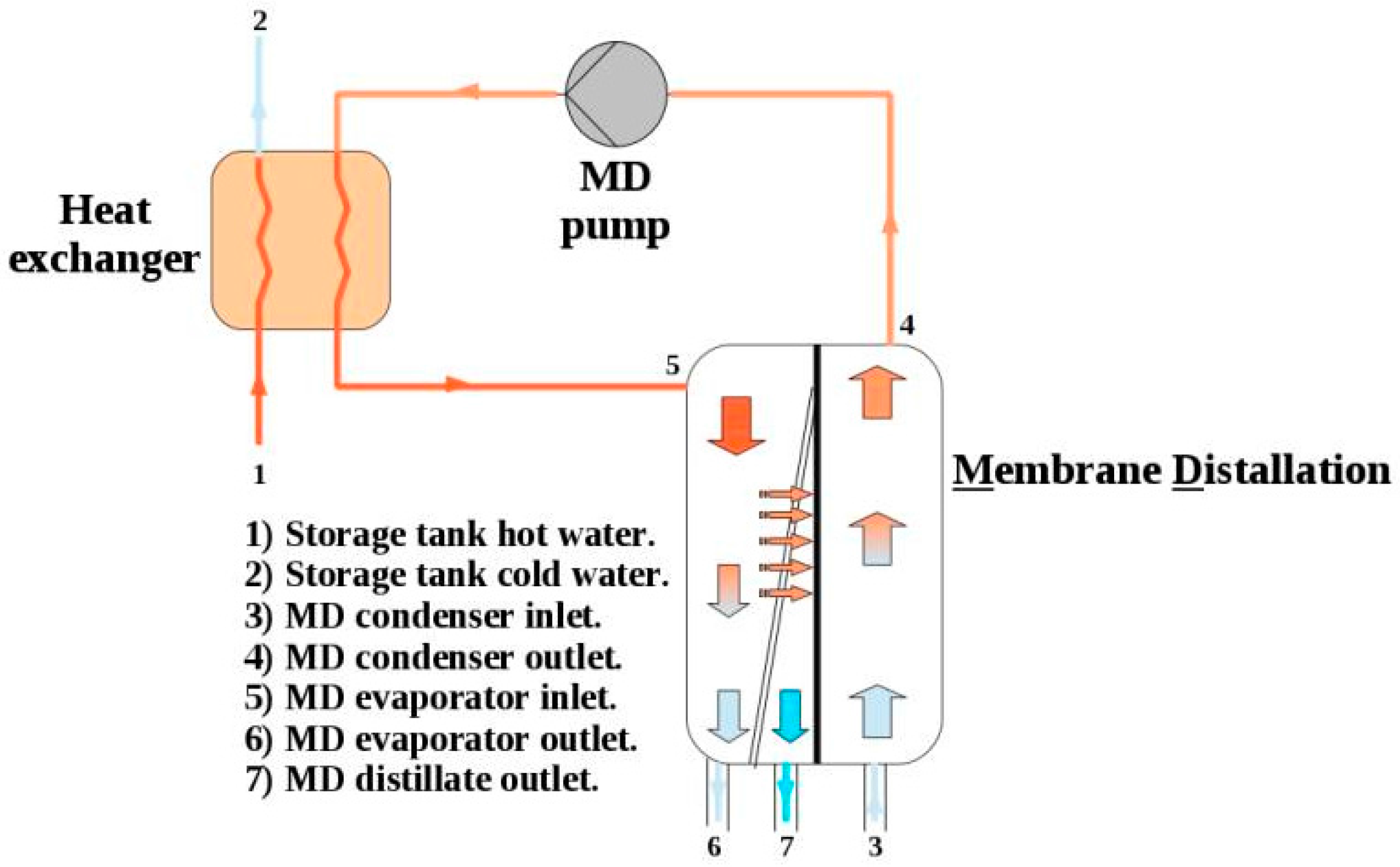
On the other hand, one of the major problems found in dry and/or isolated areas is water scarcity. The areas with the highest need of drinking water usually exhibit the highest solar energy availability [13]. Since solar energy can supply almost unlimited energy, it can be an ideal solution for distilling water in isolated areas. Membrane distillation (MD) is a non-isothermal membrane separation process used in various applications such as desalination. The feed water (sea water) does not need chemical pre-treatments, it works at atmospheric pressure, operation is flexible (continuous or intermittent operation), the process can be carried out with temperatures between about 70 and 90 °C, and solar energy can also be utilized to produce distillate by heating seawater up to that range [14]. The distillation process is based on the transport of vapor molecules through a hydrophobic micro-porous membrane [15]. Due to tension forces at the membrane surface, liquid water and any other non-volatile components cannot pass through it. Heat supplied by an external (waste) source produces some vapor from the liquid state. The difference in temperature and pressure on both sides of the membrane is the driving force which leads to vapor passing through the membrane. Then, vapor is condensed by the aid of a coolant (normally a counter flow that preheats the MD feed water), and distillation process is completed. The vapor pressure difference across the membrane which drives the MD process can be established using different configurations [16,17,18,19]:

• Direct contact membrane distillation (DCMD): is the simplest one. The membrane is in direct contact with both liquid phases (hot and cold).
• Air gap membrane distillation (AGMD): To reduce heat losses, an air gap is set between the membrane and the condensation surface. Process energy efficiency is improved but reduced distillate flows are usually obtained.
• Sweep gas membrane distillation (SGMD): Vapor is carried by a gas to an external condenser. It is usually applied to remove volatiles from the solution.
• Vacuum membrane distillation (VMD): The permeate side remains at low pressures. In some cases, vapor is condensed at a separate device.
• Permeate Gap Membrane Distillation (PGMD): Is similar to AGMD, but instead of using stagnant air, the condenser surface is full of water. The major advantage of PGMD is its energy efficiency, since an efficient heat recovery system [20,21] could be arranged.

The latter was the selected MD configuration for further modeling. Anyway, aside from the coincidence between water shortage and solar irradiation, and considering that MD is appropriate to be fed by solar energy for small capacities and isolated areas [16,22,23,24,25], distillation techniques have usually higher energy consumptions than membrane techniques like reverse osmosis (RO) or electrodialysis (ED, for brackish waters), which only consume power. Of course, power to drive the high-pressure pump of a RO unit could also be obtained from a renewable source [26], thus increasing the FW production in a hybrid scheme for seawater desalination. At present, RO processes use selective membranes which can retain most of the salt and microorganisms, leaving more than the 99% of the salts behind [13].

The hybridization of Renewable Energy System (RES) technologies has been usually utilized to provide FW in remote and arid areas. For instance, in [27] the design of a PV + WT coupled with a seawater RO unit including an energy recovery device (ERD) for a small island was generalized. In [28], the same scheme (30.8 kW_p of PV + 600 W of WT) was modeled and analyzed for desalting brackish water with RO (40 m³/day) at different locations in Tunisia. Experimental tests of the same arrangement in Israel (3.5 kW_p + 600 W) for an average production in the stand-alone brackish RO unit of 3 m³/day, can be found in [29]. If distillation units replace the RO, a multi-effect evaporator (MEE) supplied by solar and wind energy was also simulated and optimized depending on the solar collector area and system feasibility in Turkey [30].

However, hybridization in desalination is usually restricted to larger facilities. Concentrating solar power (CSP) was analyzed in the framework of a medium-scale research and development (R + D) European Project [31]. Produced steam was sent to a steam turbine (1 MW_e) that both supplied the RO system (800 m³/day) and the MED (50 m³/day) with the rejected steam. A back-up energy system (gas turbine, 1.25 MW_e) was also projected for cloudy days. For larger capacities, hybrid water desalination systems (MED + RO) supplied by conventional energy sources were optimized in [32]. A steam network with several turbines at different pressure levels was analyzed for a combined production of up to 126,300 m³/day. The same hybrid scheme supplied by a gas turbine (GT) and a combined cycle (CC) was also thermo-economically optimized in [33].

Apart from producing energy and water with hybrid techniques and RES (cogeneration schemes), there are very few examples of tri-generation or poly-generation schemes involving seawater desalination and RES. In [34,35], a poly-generation system based on PVTs, a LiBr-H₂O chiller, and a MED distiller, with a back-up biomass heater was simulated and optimized in TRNSYS^® (http://www.trnsys.com/) with weather data from Naples, Italy. A similar scheme could be optimized in its design and operation if conventional energy sources are neglected [36].

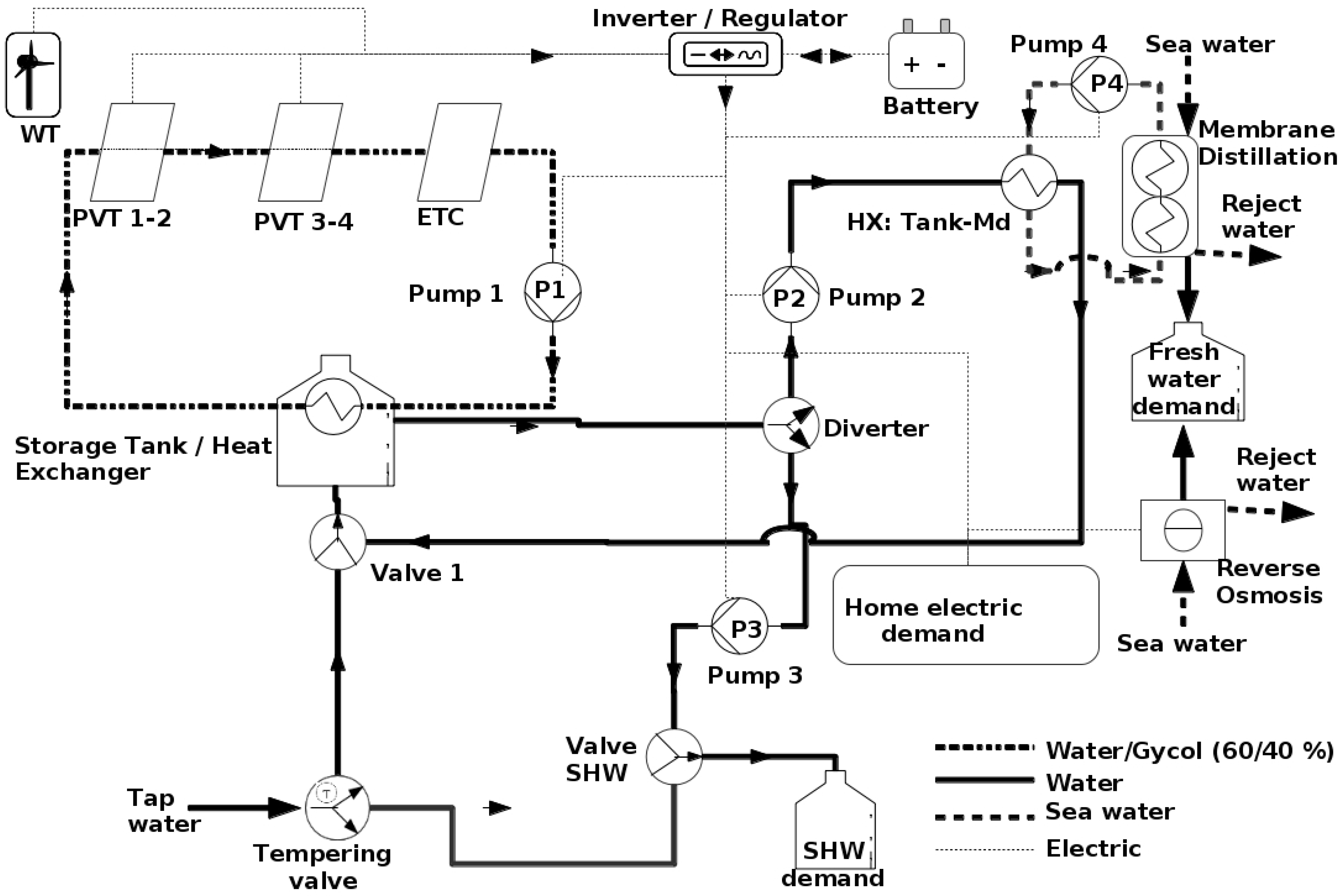
From the previous analysis, it can be observed that the combination of hybrid techniques for both RES and desalination, which also includes SHW, has not been studied in detail yet. Thus, this paper presents the design analysis of a double hybrid scheme (wind/solar + MD/RO) which allows for providing power, SHW and FW at a much reduced demand scale in isolated areas. This hybridization is a technically possible solution and its profitability will depend on alternative costs to provide water and energy by a network or local transport.

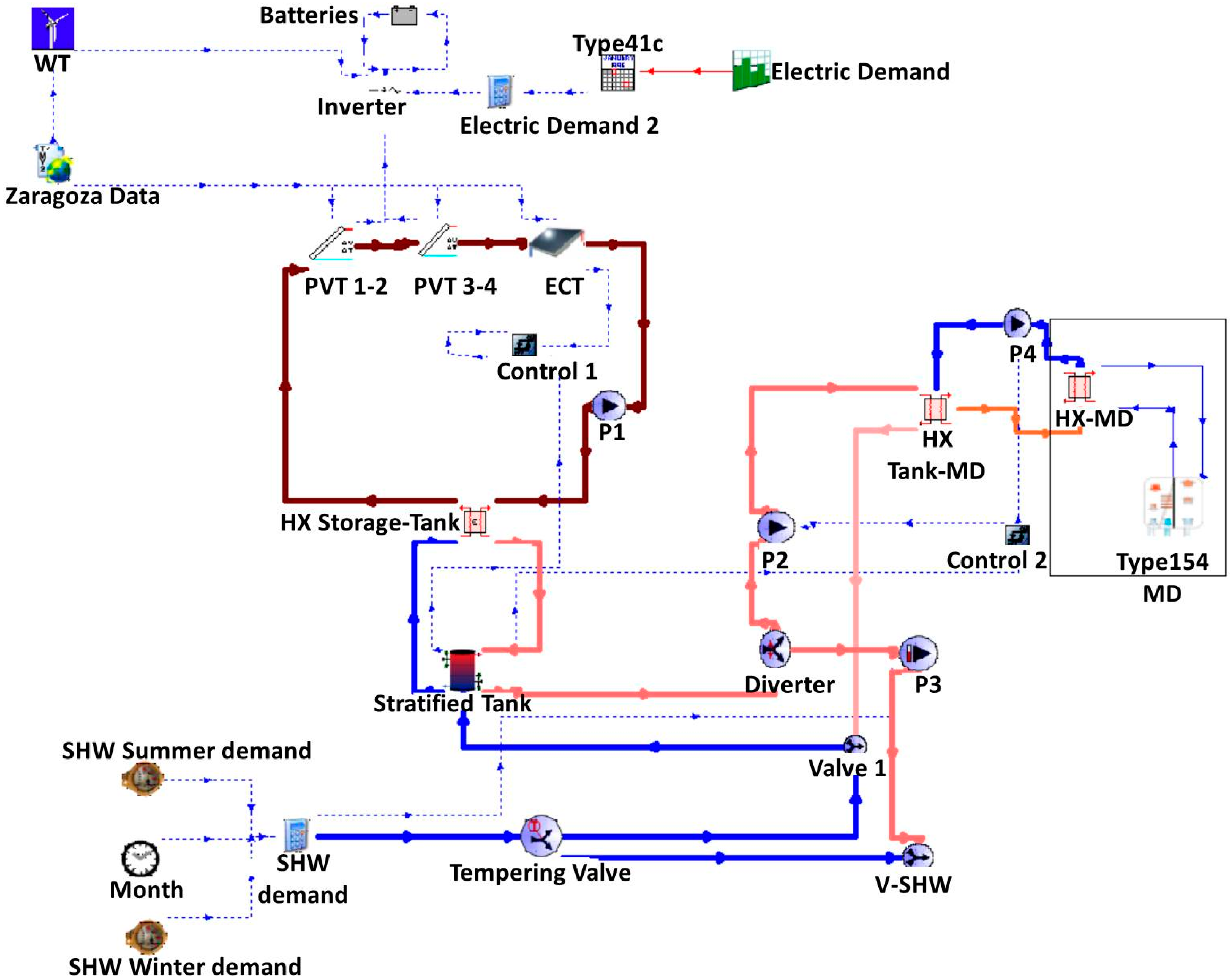
Taking into account the variability of the renewable energy sources, a dynamic simulation is required in order to model and then to assess the performance of the transient processes occurring in that scheme. Dynamic simulation of this trigeneration scheme was performed in TRNSYS^® software (v16) [37]. Its modular design easily permits to analyze main design parameters of each component but also the overall performance of the scheme proposed, according to the scheduled energy and water demands.

2. System Description

The system consists essentially of five main subsystems:

(1)

Solar loop.

(2)

SHW loop (including storage and consumption).

(3)

MD module.

(4)

RO module.

(5)

Power loop (generation, regulation, storage and consumption).

The main subsystems included in the hybrid trigeneration scheme are shown in Figure 1.

The study was carried out by using Meteonorm data base (http://www.meteonorm.com/) of a Typical Metrological Year (TMY) for the city of Zaragoza, Spain. The electric and water demand considered in this investigation were based on a single family home in Spain. The electric demand from this kind of home is about 2422.2 kWh per year [38]. The system is connected to the grid to partially supply demand when the batteries power is not enough. On the other hand, the total FW demand is estimated in 106.4 cubic meters per year, and SHW demand in 37.2 cubic meters per year [39]. Water demands are firstly covered through the storage tanks (hot water and FW), while tap water and an electrical resistance could supply the remaining demands.

2.1. Solar Loop

The solar loop consists of four PVT collectors (1.63 m² each) and one Evacuated Tube Collector (ETC) of 1.4 m². The PVTs are divided in two sets connected in series to the ETC as seen in Figure 1. Each PVT set contains two collectors in parallel. PVTs are connected to a regulator-battery system. Solar energy not converted into electricity is then transformed into thermal energy. Inside the hydraulic circuit, the water-glycol (60%/40%) fluid is sent to the storage tank by means of a heat-exchanger/pump system. According to the supplier’s recommendations, the flow rate in this circuit was set at 97.8 L/h.

2.2. Sanitary Hot Water (SHW) Loop

The hot water tank has a capacity of 325 L and is fed with tap-water. Hot water coming from the solar loop is sent to the heat exchanger inside of the tank. The tank temperature is raised to about 80 °C. Depending on that temperature and the SHW needs, two valves (V-SHW and diverter) should act to distribute the hot water flows to SHW or MD demand. Temperature of SHW served was set to 45 °C. The storage tank is also connected to a tempering valve, which regulates the final SHW temperature when hot water in the tank exceeds 45 °C.

Table 1. Monthly water demand (Fresh water demand left, sanitary hot water demand right side).

FW
Month	Total (L/Month)	Average (L/Day)
January	9314.4	300.4
February	8475.6	302.7
March	9387.4	302.8
April	9028.7	300.9
May	8732.9	281.7
Jun	8456.2	281.8
July	8692.3	280.3
August	8732.9	281.7
September	8456.2	281.8
October	8692.9	280.4
November	9067.1	302.2
December	9385.3	299.2
SHW
Month	Total (L/Month)	Average (L/Day)
January	3260.0	105.1
February	2966.4	105.9
March	3285.9	105.9
April	3159.9	105.3
May	3056.5	98.6
Jun	2959.8	98.6
July	3042.4	98.1
August	3056.6	98.6
September	2959.3	98.6
October	3042.2	98.1
November	3173.4	105.7
December	3284.9	102.4

shows the monthly water demand and the average consumption per day of FW and SHW for a typical single family home. Both demands, FW and SHW, were simulated in TRNSYS^® based on the study presented in reference [39].

On the other hand, when the tank temperature is between 70 °C and 90 °C, part of that hot water could be derived to the heat exchanger feeding the MD unit, thus activating the distillation of seawater. The maximum allowed temperature in the tank is 90 °C. This value will be regulated by the direct outfall of SHW to the sanitary network, and the use of an 8 kW air cooled condenser to cool the solar loop (not included in Figure 1).

2.3. Membrane Distillation (MD) Loop

This subsystem is divided into two loops and the MD device. From the storage tank side (hot loop), there is a pump and a heat exchanger (tank-MD) that allows transferring the heat from the hot water tank to the PGMD unit. On the other side (cold loop), the MD sub-system is connected to the same heat exchanger by means of a pump. The heat exchanged allows maintaining the vapor pressure difference to vaporize and then distill some seawater in the MD module.

Since TRNSYS^® does not have a specific MD model, a new model-type was created in its library. It is based on the modeling and experimental tests of a commercial PGMD module presented by Winter et al. [20,21], which is almost the same as the projected one in our pilot unit. The PGMD contains a spiral wound desalination membrane with a total exchange area of 10 m², a length channel of 3.5 m, a total height of 0.7 m, and a mean channel thickness of 3.2 mm. Design capacity of this MD module is 150 L/d, being its production peak around 20 L/h in the best thermal conditions. Operation of the PGMD module is presented in Figure 2 [20,40].

• Cold sea water enters in the condenser (flow 3).
• Through the condenser path, cold sea water increments its temperature due to the heat exchange with evaporator and distillate channels (flow 4).
• Sea water is heated (flow 4) by an external heat exchanger (tank-MD, flows 1–2).
• Hot sea water enters into the evaporator (flow 5). Here, some vapor is produced and the remaining liquid transfers the heat to the condenser side.
• Vapor passes through the membrane and then it is condensed to obtain the distillate (flow 7). Salinity of the remaining seawater is then slightly increased (flow 6).

2.4. Reverse Osmosis (RO) Module

This module has not been simulated in detail as a new model-type in TRNSYS^®, according to its steady performance. Only the required DC power consumption (110 W, giving an estimated production of 35 L/h and thus leading to rather low specific energy consumption for such that small RO units due to its immersed ERD) was considered, if enough discharge level was found in the batteries. The technical characteristics of the modeled RO unit are presented in

Table 2. RO technical characteristics [41].

Description	Characteristic Value
Nominal feed water salinity	35,000 ppm
Nominal temperature	25 °C
Fresh water production	35 L/h
Quality of water produced	300 ppm
Salt rejection	99.14%
Power consumption	110 W

.

2.5. Power Loop

Power generated in the PVT subsystem (4 × 240 W_p) is driven to a regulator which is responsible for managing the charge and discharge of the battery. The WT was simulated in TRNSYS^® through a numerical model that adjusts the power-velocity curve of a commercial model (400 W_p) [42]. This unit is also connected to the regulator. A set of two batteries (250 Ah and 12 V) connected in series accumulates that power for further needs. Electric demand consists of the power required by three 5 W AC pumps (pump 1 in the solar loop, pump 2 for the hot water to MD heat exchanger, and pump 3 for SHW), the 10 W DC pump used by the MD loop, and finally the power consumed by the RO (110 W, DC). Any remaining power could be used to partially cover the domestic power demand or stored in the batteries. Daily electric demand for a typical dwelling was simulated according to standards [38].

Table 3. Electric demand from a single family home.

Home Demand
Month	Total (kWh/Month)	Average (Wh/Day)
January	205.4	6626.8
February	186.4	6657.4
March	207.0	6678.1
April	199.4	6646.7
May	206.0	6646.3
Jun	200.2	6673.6
July	206.2	6652.1
August	206.0	6646.3
September	200.2	6673.6
October	206.2	6652.1
November	199.3	6644.4
December	206.5	6658.3

shows the monthly electric demands for a single family home as well as the average energy consumption per day implemented in TRNSYS^® simulation.

The whole system has been divided in five subsystems. (1) The solar loop, where solar energy is collected and transformed into thermal energy and electricity; (2) SHW, where thermal energy is delivered to the tap water to increase its temperature; (3) MD; (4) RO; and (5) Power loop.

Table 4. Subsystems simulated in TRNSYS^®. * (RO was not modeled as a new model-type).

Sub-System	Units, Size
Solar Loop	Four PVT collectors, 1.63 m2 at 40°
	One ETC, 1.4 m2
	One AC pump, 5 W
SHW	One tank with internal heat exchanger, 325 L
	One diverter valve
	One T valve (V-SHW)
	One AC pump, 5 W
	One tempering valve
MD	PGMD spiral wound distillation module, maximum distillate 20 L/h
	One AC pump (heat exchanger), 5 W
	One DC pump (MD system), 10 W
	One counter-flow heat exchanger
RO *	Reverse Osmosis unit, 110 W, permeate 35 L/h
Power Loop	Four PVT collectors, 240 Wp
	One wind turbine, 400 Wp
	Two batteries, 250 Ah and 24 V

shows these five subsystems and the main units for the proposed design (base case).

3. Dynamic Model

By unifying all subsystems presented in Section 2, the complete dynamic simulation could be performed in TRNSYS^®. This allows not only to optimize the components and parameters, but also to find possible errors in the preliminary system design, according to the annual coverage rate of power, SHW and FW demands.

3.1. Project Creation

Figure 3 shows the complete project created with TRNSYS^®.

The TRNSYS^® project started with meteorological data from the place where the trigeneration system was established. In this case, Zaragoza city, located in the northeast of Spain, was the chosen one. As previously mentioned, data were obtained from Meteonorm data base and has been introduced in TRNSYS^® as a file-input. Figure 4 shows the behavior of solar radiation (40° tilt), wind velocity at WT height (13 m) and ambient temperature along the year at Zaragoza, Spain.

The simulation was carried out in a complete year having a time step of 12 min. To complete a simulation, 43,800 iterations were usually required.

PVT and ETC collectors were linked to the meteorological input data (solar radiation, ambient temperature and wind velocity). PVTs and ETC were physically interconnected by means of a pump to a heat exchanger, thereby transferring the recovered thermal energy to a stratified tank. A control system (control 1) was connected to the pump, the tank and the ETC collector to induce a hysteresis cycle which allows the adequate regulation of the tank temperature.

In order to adequately manage the SHW produced, hot water in the tank is sent to valve V-SHW through a diverter valve and a pump P3. The demand is managed by a tempering valve which splits two tap-water flows:

(1)

Refilling storage tank water: If SHW is extracted from the storage tank, the same amount of water has to be replaced with cold tap-water. Water is recovered in storage tank through valve 1.

(2)

Tempering water: That second flow only exists if the tank temperature exceeds 45 °C. The tempering valve computes the energy and mass balance to serve SHW at that service temperature.

Apart from the SHW service, if the tank temperature is above 70 °C, this hot water is ready to feed the MD via its heat exchanger (tank-MD). In this service, hot water leaves the storage tank, then passes through the diverter zone, pump P2 and finally returns to the tank through valve 1. The pump and the MD system were controlled with the unit control 2 as it can be seen in Figure 3.

The MD module was then interconnected with the heat exchanger (tank-MD) by a pump P4. The MD type included a MD model aided by an external heat exchanger (HX-MD as can be seen in Figure 3). Therefore, in combination both MD and HX-MD operate as a unique MD unit.

On the other hand, electric energy produced by PVTs and WT was managed in a battery-regulator/inverter system. The micro-WT was also modeled from updated existing TYPE90. WT type was optimized by introducing the power production characteristic curve from manufacturer [42]. Power demand was modeled including domestic and RO consumptions as external demands.

3.2. Standard TRNSYS^® Types

All units and their respective types used in the simulation are presented in

Table 5. Units and Types simulated in TRNSYS^®.

Unit	Type
Meteorological data	109-TMYZ
PVTs	50b
ETC	1a
WT	90
Pumps P1, P2 and P4	114
Pump P3	110
-Heat exchanger inside of storage tank -Heat exchanger between storage tank and MD	91
Storage tank	40c
Heat exchanger inside of MD	5b
MD	154-MD
Control 1 and 2	2b
SHW demand	14b and 21
-Valve SHW -Valve 1	11h
Diverter	11f
Tempering valve	11b
Inverter	48b
Battery	47a
Electric demand	41c and 14h

. TYPE109-TMY2 reads and process weather data along the complete simulation. The energy from the solar loop is transferred to the stratified tank by means of TYPE91, which is a heat exchanger that operates to calculate the maximum possible heat transfer with a constant effectiveness of 0.9. The same model type has been used to simulate the heat transfer between the storage tank and the MD system.

TYPE40c is a stratified tank that consists of four fully-mixed equal volume segments. The total volume of this storage tank is 0.325 m³. The control system type utilized in the simulation is the TYPE2b which is an off/on differential controller, the value of this control type is defined by the difference of upper and lower temperatures of the tank-solar loop and for the temperatures between the storage tank and MD system.

The SHW demand is created by two types: TYPE14b that generates a time dependent forcing function for 24 h of the day, and TYPE21 that creates the SHW demand depending on the current time in the simulation.

Water flows are distributed (diverted or mixed flows) by means of TYPE11. This type has been used in different modes: h, f, and b. In all cases the type performs the mass balance and controls the thermal systems by means of an energy balance.

The electric simulation consists of four types. TYPE48b is a regulator/inverter which distributes DC power from the PVT array to and from battery. This type also converts DC power to AC and sends it to the load. Type47a models a lead-acid storage battery, it computes battery rate of charge and discharge. Finally the electric demand is created by TYPE14h which produce an electric demand forcing function along a single day (24 h) and TYPE41c that organizes the daily profiles generated by TYPE14h into an annual profile.

3.2.1. Photovoltaic/Thermal (PVT) Model

PVT collectors were modeled with TYPE50b. In this type, the well-known Hottel-Whiller equation for thermal analysis of flat-plate collectors is extended to combine both, thermal and photovoltaic collector. The calculation performed by the type is a simple modification of the conventional parameters of the original model. This type assumes that the electrical conversion efficiency is a linear decreasing function of the local absorber temperature [43].

The model is divided in two parts [4], the photo-thermal and the photo-electric part. In the first part, the efficiency of the energy collected is estimated by applying the Hottel-Whillier equation:

$$\mathsf{\eta }={\left(\mathsf{\tau }\mathsf{\alpha }\right)}_e-U_L\left(\frac{T_p-T_a}{G_t}\right)$$

(1)

The first right side term is the effective product between the transparent cover transmittance and the absorption, where U_L is the total heat loss coefficient (W/m²-K), T_p and T_a are the PVT rear panel temperature and the ambient temperature respectively, both in °C. Finally, G_t is the solar radiation in W/m².

On the other hand, the photovoltaic efficiency can be estimated by the ratio between the electric energy output (E in W) and the solar radiation (G_t in W/m²) over the PVT area (A_PVT in m²):

$${\mathsf{\eta }}_e=\left(\frac{E}{A_{PVT}{G}_t}\right)={\mathsf{\eta }}_o-\frac{C_1\left(T_p-T_a\right)-C_2{\left(T_p-T_a\right)}^2}{G_t}$$

(2)

where η_o is the optical performance of the PVT, C₁ and C₂ are the thermal losses coefficients set as 2.59 W/m²-K and 0.012 W/m²-K² respectively [44].

TRNSYS^® PVT model has been validated by Sardabaradi et al. [45]. This validation was demonstrated by comparing predicted collector’s outlet temperature changes and daily system efficiencies with measured data acquired from an experimental bench test at Ferdowsi University of Mashhad. It was found that there is less than 3% of uncertainty in all measured data and calculated parameters. The authors found differences of about 2.1% in electrical power output and only 1% in collector’s outlet fluid temperatures when comparing TRNSYS^® simulation and the bench test.

3.2.2. Evacuated Tube Collector (ETC) Model

An ETC is a heat exchanger that transforms solar radiation energy into internal energy of the circulating water/glycol flow. It transfers energy from the incident and diffuse solar radiation to working fluid. The type selected to simulate this unit was TYPE1a. The efficiency of this type is based on the Hottel-Whiller-Bliss equation as presented next [46]:

$$\mathsf{\eta }=F_R{\left(\mathsf{\tau }\mathsf{\alpha }\right)}_e-F_R{U}_L\left(\frac{T_p-T_a}{G_t}\right)-F_R{U}_L{\left(\frac{T_p-T_a}{G_t}\right)}^2$$

(3)

Here F_R is the overall collector heat removal efficiency factor, which can be reformulated as:

$$\mathsf{\eta }=A_0-A_1\left(\frac{T_p-T_a}{G_t}\right)-A_2{\left(\frac{T_p-T_a}{G_t}\right)}^2$$

(4)

However, the most common method to define the performance of this kind of collectors is by computing the useful thermal energy (Q_u) transferred from the radiation to the fluid flow passing through the ETC in W (energy gain of the working fluid):

$${\dot{Q}}_u={\dot{m}}_{wg}{C}_{Pwg}\left(T_{wg-in}-T_{wg-out}\right)$$

(5)

where the subscript wg represents the working fluid (water/glycol), m the mass flow rate kg/s, C_p the heat capacity (3572.5 J/kg-K) and T_wg the temperature of the working fluid entering and leaving the ETC [44].

The ETC model has been validated in [47], where authors have demonstrated that the discrepancy in predicting collector outlet temperature is about 13% compared with experimental results. On the other hand, Ayompe et al. [48] have also computed a 13% in outlet temperature the found differences between simulation and real system. Finally, the error calculated in the accumulated collector energy was 12%.

3.2.3. Circulation Pumps Model

TRNSYS^® component TYPE114 is used to circulate water at three different stages of the complete cycle: solar loop, storage tank to MD heat exchanger, and fluid circulation inside the MD system.

• Pump in the solar loop works at a flow rate of 0.027 kg/s of water/glycol.
• Pump between the storage tank and the MD heat exchanger moves hot water at 0.055 kg/s.
• Pump of the MD system has a flow rate of 0.055 kg/s of sea water.

This type computes the increment in the output temperature as:

$$\left(T_{in}-T_{out}\right)=\frac{Q_f}{m_f{C}_p}$$

(6)

T_in and T_out are the entering and leaving the pump in °C, m_f is the flow rate in kg/s, and Q_f is the thermal energy transferred from the pump motor to the fluid flow passing through the pump in W. The energy transferred to the fluid is defined by Equation (7):

$${\dot{Q}}_f=P_s\left(1-{\mathsf{\eta }}_p\right)+\left(P-P_s\right)f_m$$

(7)

where P_s is the pumping shaft power in W, η_p the efficiency of the pumping, P is the input power in W, and f_m is the fraction of pump inefficiencies that contribute to a temperature rise of the working fluid [44].

On the other hand, a variable speed pump TYPE110 has been selected to serve the SHW. The fact that the SHW production is not constant along the whole day allows effective use of a variable speed pump.

Equation (6) of TYPE114 coincides with TYPE110. However, there is a simplification in the energy transferred from the pump to the fluid flow as shown in Equation (8):

$${\dot{Q}}_f=P{f}_m$$

(8)

3.2.4. Membrane Distillation Model

PGMD system was simulated through new a type called TYPE154 [20,21]. This type was generated following the information presented in [1,2,3,4,5,6,7,8,9,10,11,12,13,14,15,16,17,18,19,20,21,22,23,24,25,26,27,28,29,30,31,32,33,34,35,36,37,38,39,40,41,42,43,44,45,46,47,48,49], with the aid of G95 open source FORTRAN compiler [50]. The model is based on empirical relation (1st order polynomial) for the distillate water production expressed as a function of the sea water flow rate (0.055 kg/s) and steady operation temperatures (salinity of 50 g/kg, condenser inlet temperature T_ci = 25 °C and evaporator inlet temperature T_ei = 80 °C). Figure 5 shows the comparison between the model obtained for TRNSYS^® TYPE154 and the model presented in references [20,21].

Since there is a very similar behavior between the proposed TRNSYS^® type and the model from the reference, TYPE154 can be used to estimate the production of the specific MD system presented in Section 2.3. That is, it can be used to predict the PGMD FW production within Equation (9) and the next operating conditions: feed water range 0.055–0.13 kg/s, T_ci range 20–40 °C and T_ei range 70–80 °C.

Figure 6 shows an example of typical PGMD production curves for different scenarios created:

$${\dot{m}}_{freshwater}=-5.48+0.043{\dot{m}}_{feedwater}+0.079\left(T_{ei}-T_{ci}\right)$$

(9)

4. Simulation Results

4.1. Pre-Design System Evaluation (Base Case)

In this section, some operational parameters such as temperatures and electricity, SHW and desalted water produced are analyzed for the preliminary design of the hybrid-trigeneration scheme. To facilitate the interpretation of those results, all graphics are presented in a monthly and daily basis.

The comparison between demand (red) and SHW production (blue) in Figure 7 shows that more than the 95% of the SHW demand can be covered along the whole year. Only in winter season the tank temperature does not reach the service temperature (45 °C) for SHW use until 10 a.m., as can be seen in the typical winter day graphic on Figure 7. Selected winter and summer days were respectively 18 December and 19 July (Figure 7).

Evolution of the tank temperature shows its minimum (35 °C) at the beginning and the end of the year, but averaged temperatures vary from 60 °C to 90 °C. On the other hand, and due to the efficient tempering valve included in the scheme, SHW temperature oscillates between 45 °C and 46 °C along the whole year except in December when, due to low temperatures and the lack of radiation, the SHW temperature decreases until 30 °C. Tank and SWH average temperatures are presented in Figure 8, as well as those ones for a typical winter day (18 December) and summer day (19 July).

FW distilled in the MD unit can be seen in Figure 9. Distillate is concentrated in summer season, when the storage tank temperature is usually below the threshold (70 °C) that activates the MD system. Figure 9 shows the yearly production and the detail for a typical winter and summer day.

Power coming from the PVT loop and the WT is firstly consumed by the internal demand (pumps and RO) and then external (home demand) should be partly covered. Nevertheless, in Figure 10 it is shown that the 70% of the total electric demand can be covered: this means that AC and DC pumps can operate in a standalone state during the whole year, but some energy has to be delivered from the grid in order to fully cover the demand.

The WT production highly depends on the wind velocity computed for each month. As can be seen in Figure 4, averaged wind velocity in Zaragoza, Spain is almost constant for the whole year (5 m/s) with small variations in April and October. Those variations are translated in the WT production (Figure 10) since April is the month with the highest production (28% more than the average) and October the month with the smallest production (34% less than the average).

On the other hand,

Table 6. Allowed productions and covered demands in the base case.

Product	Production	Demand	Coverage Ratio
SHW	36,990 L	37,247 L	99.3%
FW (MD + RO)	15,311 + 306,607 L	106,421 L	302%
Electricity	1890 kWh	2711 kWh	70%

shows the annual production of SHW, FW and electricity for the base case of this preliminary design.

Note that FW production is higher than the demand. Thus, the RO unit should be partly turned off at night, or alternatively some amount of water could be sold or stored for further peak demands.

4.2. Parametric Simulation

In order to improve the first design, production of SHW, FW (mainly the produced by the MD unit) and electricity is expected to rise up as much as possible. Six free-design variables of the first scheme were independently varied in the TRNSYS^® model. The unit capacities are only incremented in cases 2 (ETC area), 3 (storage tank capacity), and 6 (battery capacity):

• Case 1 (Collector slope): the collectors tilt was analyzed for two additional cases, at 30° and 50°.
• Case 2 (Evacuated tubes solar collector area): six vacuum tubes were added to the initial ETC composed by 14 vacuum tubes. The area was then increased up to 2 m².
• Case 3 (Storage tank capacity): was increased up to 0.45 m³ and 0.5 m³ respectively.
• Case 4 (MD flow rates): flow to heat and internal flow of the MD were varied as presented in

  Table 7. Parametric simulations of some free-design variables in the scheme.

  Case	Collector Slope (°)	ETC Area (m2)	Storage Tank Volume (L)	MD-Heat Exchanger Flow (L/h)	MD Inlet Flow (L/h)	SHW Demand (%)	Battery Capacity (Ah)
  Base	40	1.4	325	200	200	100	250
  Case 1-1	30	1.4	325	200	200	100	250
  Case 1-2	50	1.4	325	200	200	100	250
  Case 2	40	2	325	200	200	100	250
  Case 3-1	40	1.4	450	200	200	100	250
  Case 3-2	40	1.4	500	200	200	100	250
  Case 4-1	40	1.4	325	200	400	100	250
  Case 4-2	40	1.4	325	400	400	100	250
  Case 4-3	40	1.4	325	200	500	100	250
  Case 4-4	40	1.4	325	500	500	100	250
  Case 5-1	40	1.4	325	200	200	40	250
  Case 5-2	40	1.4	325	200	200	20	250
  Case 6-1	40	1.4	325	200	200	100	180
  Case 6-2	40	1.4	325	200	200	100	300

  .
• Case 5 (Use of SHW): SHW production was decreased by 60% and 80% respectively, in order to maximize FW production in the MD unit.
• Case 6 (Battery capacity): it was varied up to 180 and 300 Ah.

Table 7 presents the set of alternative design variables analyzed.

Results indicate that the electricity production is similar in all parametric simulations. The maximum increment (7%) was found in case 4-4. This can be seen in Figure 11.

The SHW production remains almost constant in all cases, except for case 5 where it was deliberately decreased. It can be observed in Figure 11 and

Table 8. Yearly productions table in the sensitivity analysis.

Production	MD (L)	RO (L)	SHW (L)	Electricity (kWh)
Base	15,311	306,607	36,990	1890.37
Case 1-1	15,352	306,607	36,803	1898.82
Case 1-2	14,544	306,607	37,013	1865.52
Case 2	16,993	306,607	37,121	18,628.0
Case 3-1	16,489	366,607	37,090	1904.45
Case 3-2	16,932	306,607	37,146	1907.78
Case 4-1	16,839	306,607	36,769	1983.59
Case 4-2	16,824	306,607	36,899	1984.38
Case 4-3	18,103.5	306,607	36,870	2015.77
Case 4-4	18,164.6	306,607	36,878	2016.11
Case 5-1	17,508.0	306,607	14,902	1848.36
Case 5-2	18,454.8	306,607	7460	1836.08
Case 6-1	15,334.8	306,607	36,912	1893.57
Case 6-2	15,300.9	306,607	36,921	1893.77

that if the SHW demand is not covered, distillate in the MD could be then increased. In case 5-1, an increment of 14% in the MD production was found when the SHW production decreased by 60%. The same happens in case 5-2, varying SHW production by 80% supposes an increment of 21% in the MD. However, similar effects can be found in cases 4-3 and 4-4, when the internal MD flow was set to 400 L/h or 500 L/h, since additional 18% and 19% of distillate were respectively found, with no significant impact on the SHW production: they correspond to a reduced flow delivered to the MD unit that also leaves to serve the SHW use. It should be noted that the increment of production by increasing the storage size for cases 3 and 6 is not significant compared with those results obtained in the base case.

Finally, and as expected, increasing the ETC area from 1.4 to 2 m² (Case 2) would lead to a increase in the distillate by 11.4%, while keeping almost the same electricity and the SHW production. In the rest of parametric studies, no noteworthy production increments were found.

From these results, it can be inferred that the best design case (i.e., following the maximum MD distillation) could be made by increasing the ETC area and the MD internal flow. A definite scheme based on case 2 and case 4-4 is then proposed in

Table 9. Best case design (maximum MD production).

Case	Collector Slope (°)	ETC Area (m2)	Storage Tank Volume (L)	MD-Heat Exchanger Flow (L/h)	MD Inside Flow (L/h)	SHW Production (%)
Base	40	1.4	325	200	200	100
Case 2/4-4	40	2	325	500	500	100

as the best design (case 2/4-4).

Regarding the flow operating in the MD, the results obtained completely agree with the results presented in [21] under steady conditions in the range of 25–80 °C for 90 min. In that reference, the MD could continuously produce about 9 L/h with an inlet flow rate of 200 L/h, and when this flow rate was incremented to 500 L/h, the production was augmented up to 22 L/h. If similar conditions are selected in our transient model (i.e., similar time lapse, and the same temperatures for the seawater entering the MD condenser and evaporator sides), distillate flow obtained by the model is very close to the later, as it can be seen in Figure 12.

If the yearly production is compared, in that case the overall production in the MD is incremented in 35.4% when the inlet MD flow increased from 200 L/h to 500 L/h, as seen in Figure 13.

Annual average distillate MD production of the optimal scheme is 56.8 L/d, being 41 L/d in the base case.

Table 10. Results comparison between base and optimum (MD) case.

Case	SHW		FW (MD)		FW (RO)		Electricity
Base case	36,990 L	100%	15,311 L	100%	306,607 L	100%	1890 kWh	100%
Case 2/4-4	37,100 L	100.3%	20,745 L	135%	306,607 L	100%	1997 kWh	107%

shows the main production gaps between the base and the optimum case.

4.3. Daily Analysis

This comparative analysis has now been focused on the averaged day of every month in the hybrid trigeneration system.

First, the SHW production is shown in Figure 14a. It can be observed that, in general, there are not significant differences between the base case and the case 2/4-4. The same happens with the electricity production Figure 14b. However, great differences are found in the FW production.

Contrary to the SHW and electricity productions, MD distillate is not continuously produced along the year. As it was restricted by the storage tank temperature (70 °C), in winter season thermal energy collected by the PVT and ETC is not usually enough to produce distillate.

Table 11. MD non-operational days.

Case	Jan.	Feb.	Mar.	Apr.	May	Jun.	Jul.	Aug.	Sep.	Oct.	Nov.	Dec.
Base case	22	14	11	8	4	4	2	2	2	9	21	27
Case 2/4-4	22	15	10	9	4	5	2	2	2	6	19	26

shows the number of days per month in which the MD module was not activated in a typical year.

Between November and February, the MD system is not able to produce distillate in more than 20 days those months. Fortunately, in the rest of the months of the year, only on 2 days water will be produced merely by RO. It should be noted that averaged meteorological data are used in TRNSYS^®, but in a clear and sunny day higher irradiation than forecasted will surely occur.

MD production is shown in Figure 15. During the winter season, distillate production per day is 27% higher in the best case with respect to the base one. In summer, the production is 47% higher per day. Some other alternatives to increase MD distillate should be to reduce the SHW demand, which were tested in cases 5, or operate the MD at even lower activation temperatures (e.g., 60 °C in the tank), besides of the low distillate flows predicted at those conditions by the models [18].

Finally, Figure 16 shows the evolution of the MD production in one summer day (July) and in one winter day (November). These results are also based on the averaged day of those months. It can be seen that during summer, the MD system operates continuously during 8 h (from 10 a.m. to 19 p.m.).

In winter, the FW production starts at noon and produces 3.5 h, later stops 10 min and then re-operates again for one hour more. This is provoked by the typical SHW demand at noon, which cools the water tank and does not allow feed the MD unit for a short period.

5. Economic Analysis

A simple economic feasibility study of the hybrid plant is presented in this section. To assess the costs of desalted water, SHW and power, the investment costs of the devices associated to the generation of each product were taken into account. For instance, investment costs of the MD and RO units were used to estimate water costs. Regarding SHW, a portion of PVT, the ETC, water tank, pumps and regulation valves were considered. Finally, to account for the power costs, the investment required in PVT, WT, batteries and regulator-inverter was introduced. The life cycle assumed for all devices was 20 years.

Table 12. Cost estimation in the sensitivity analysis.

Case Study	Water (€/m3)	SHW (€/m3)	Electricity (kWh)
Base	3.20	3.78	0.106
Case 1-1	3.20	3.80	0.105
Case 1-2	3.21	3.78	0.107
Case 2	3.16	3.78	0.105
Case 3-1	3.19	4.04	0.105
Case 3-2	3.18	4.11	0.105
Case 4-1	3.18	3.81	0.101
Case 4-2	3.18	3.79	0.101
Case 4-3	3.17	3.80	0.099
Case 4-4	3.17	3.80	0.099
Case 5-1	3.18	7.05	0.108
Case 5-2	3.17	12.73	0.109
Case 6-1	3.20	3.79	0.100
Case 6-2	3.20	3.79	0.111
Case 2/4-4	3.15	3.84	0.100

shows those costs for the parametric study included in Section 4.2.

Economic optimum for all the products does not coincide with the optimum presented in Section 4.2 (case 2/4-4), since this case was defined as the highest water producer, especially by means of the MD unit. Thus, and it was expected, the lowest water cost was found in that case. Regarding power costs, the increase of ETC area allows operating the PVTs at lower temperatures and therefore higher efficiencies that gave major generation of power along the year. This is translated into a low generation cost in this option, but not the least. Finally, as ETC area increased the investment cost associated to SHW did so too, but no significant production was found in that case, taking into account that additional thermal energy is dedicated to produce more desalted water in the MD.

6. Conclusions

A small pilot plant consisting of two renewable energy devices (PVT and WT) providing power and SHW, as well as two FW desalting technologies (MD and RO), has been carefully modeled here. Only commercial devices were used in the design analysis. The case study was adapted for the city of Zaragoza, Spain. The transient simulation software TRNSYS^® version 16 was used for this purpose. This software has been proved as a powerful tool to simulate the trigeneration installation during the design stage, since it allows assessing the overall performance of the system along a complete year. As TRNSYS^® was not designed to model distillation or desalination processes, it was necessary to create a new type to achieve the complete simulation. The model presented here agreed with that one presented in reference [21] if operation is compared at similar steady conditions, which corresponds to the same commercial spiral-wound MD-module.

Results show that the optimum scheme found could provide most of the power, SHW and water demands for an isolated single family home as follows:

• The base case analyzed is able to cover up to 70% of electric demand; this coverage ratio is incremented to 75% when the optimum case 2/4-4 is simulated. However, it has to be taken into account that the RO was scheduled to work continuously, thus exceeding by 200% the FW demand required. That is, some surplus energy is stored in form of desalted water, what is, at the end, the third way to manage the balance between the renewable energy availability and user demands.
• Since the proposed WT increases in 30% the total power production, an additional WT of 400 W_p could be the definite solution for the full coverage of the family home.
• Sensitivity analysis of six free-design variables showed that SHW and electricity production remained almost constant in all parametric studies. Thus, the optimization was concentrated in the maximization of the MD distiller. This was found by varying the tank temperature or the flow rate operating in the MD.
• SHW is the same in base case and optimum case. However, a 7% power production increment was found in optimum case with respect the base case.
• The optimum case increased a lot the MD production. Distillate from the MD system was increased by 35% from 15,311 liters per year to 20,745 liters per year.
• Water, SHW and power costs found in the optimum case are around 3.15 €/m³, 3.84 €/m³ and 0.10 €/kWh respectively, making this scheme a feasible alternative for small isolated family homes.

This work is the first step in a more ambitious project including a small hybrid-trigeneration pilot plant, which has been erected at the University of Zaragoza based on the main results obtained in this paper. Specifically, a control temperature that splits the use of hot water to feed the MD or to cover the SHW demand will be carefully analyzed in the field tests, according to important variations found in the simulations performed.

References

1. Galiana, E. Solar Collector Bench Test Simulated by TRNSYS®. New Types Implementation. Bachelor’s Thesis, Polytechnic University of Cartagena, Cartagena, Spain, 2009. [Google Scholar]
2. Trujillo, A.; Domínguez, I.; Herrera, T. Using TRNSYS® simulation to optimize the design of a solar water distillation system. Energy Proc. 2014, 57, 2441–2450. [Google Scholar] [CrossRef]
3. EurObserv’ER. Solar Thermal and Concentrated Solar Power Barometer; European Union Report; Observ’ER: Paris, France, 2014. [Google Scholar]
4. Liang, R.; Zhang, J.; Zhou, C. Dynamic simulation of a novel solar heating system based on hybrid photovoltaic/thermal collectors (PVT). Proc. Eng. 2015, 121, 675–683. [Google Scholar] [CrossRef]
5. Astea, N.; Pero, C.; Leonforte, F. Optimization of solar thermal fraction in PVT systems. Energy Proc. 2012, 30, 8–18. [Google Scholar] [CrossRef]
6. Hauranta, P.; Ménézo, C.; Gaillard, L.; Dupeyrat, P. A numerical model of a solar domestic hot water system integrating hybrid photovoltaic/thermal collectors. Energy Proc. 2015, 78, 1991–1997. [Google Scholar] [CrossRef]
7. Astea, N.; Leonforte, F.; Pero, C. Design, modeling and performance monitoring of a photovoltaic-thermal (PVT) water collector. Sol. Energy 2015, 112, 85–99. [Google Scholar] [CrossRef]
8. Buonomano, A.; Calise, F.; Vicidomini, M. Design, simulation and experimental investigation of a solar system based on PV panels and PVT collectors. Energies 2016, 9, 497. [Google Scholar] [CrossRef]
9. Tina, G.; Grasso, A.; Gagliano, A. Monitoring of solar cogenerative PVT power plants: Overview and a practical example. Sustain. Energy Technol. Assess. 2015, 10, 90–101. [Google Scholar] [CrossRef]
10. Tummala, A.; Velamati, R. A review on small scale wind turbines. Renew. Sustain. Energy Rev. 2016, 56, 1351–1371. [Google Scholar] [CrossRef]
11. Bakic, V.; Pezo, M.; Stevanovic, Z.; Zivkovic, M.; Grubor, B. Dynamical simulation of PV/wind hybrid energy conversion system. Energy 2012, 45, 324–328. [Google Scholar] [CrossRef]
12. Huang, Q.; Shi, Y.; Wang, Y.; Lu, L.; Cui, Y. Multi-turbine wind-solar hybrid system. Renew. Energy 2015, 76, 401–407. [Google Scholar] [CrossRef]
13. Rym, C.; Dhaouadi, H.; Mhiri, H.; Bournot, P. A TRNSYS® Dynamic Simulation Model for Photovoltaic System Powering a Reverse Osmosis Desalination Unit with Solar Energy. Int. J. Chem. React. Eng. 2010, 8, 1–13. [Google Scholar]
14. Raluy, R.; Schwantes, R.; Subiela, V.; Peñate, B.; Melián, G.; Betancort, J. Operational experience of a solar membrane distillation demonstration plant in Pozo Izquierdo-Gran Canaria Island (Spain). Desalination 2012, 290, 1–13. [Google Scholar] [CrossRef]
15. Khayet, M. Membranes and theoretical modeling of membrane distillation: A review. Adv. Colloid Interface Sci. 2011, 164, 56–88. [Google Scholar] [CrossRef] [PubMed]
16. Zaragoza, G.; Aguirre, A.; Burrieza, E. Efficiency in the use of solar thermal energy of small membrane desalination systems for decentralized water production. Appl. Energy 2014, 130, 491–499. [Google Scholar] [CrossRef]
17. Camacho, L.; Dumée, L.; Zhang, J.; Li, J.; Duke, M.; Gomez, J.; Gray, S. Advances in membrane distillation for water desalination and purification applications. Water 2013, 5, 94–196. [Google Scholar] [CrossRef]
18. Onsekizoglu, P. Membrane Distillation: Principle, advances, limitations and future prospects in food industry. In Distillation—Advances from Modeling to Applications; Zereshk, S., Ed.; InTech: Rijeka, Croatia, 2012; pp. 233–267. [Google Scholar]
19. Jansen, A.; Assink, W.; Hanemaaijer, J.; Medevoort, J. Membrane Distillation—Producing High Quality Water From Saline Streams by Deploying Waste Heat. Available online: https://www.tno.nl/media/1509/membrane_distillation.pdf (accessed on 29 February 2016).
20. Winter, D.; Koschikowsky, J.; Ripperger, S. Desalination usuing membrane distillation: Flux enhancement by feed wate deaeration on spiral-wound modules. J. Membr. Sci. 2012, 243, 215–224. [Google Scholar] [CrossRef]
21. Winter, D.; Koschikowsky, J.; Wieghaus, M. Desalination using membrane distillation: Experimental studies on full scale spiral wound modules. J. Membr. Sci. 2011, 375, 104–112. [Google Scholar] [CrossRef]
22. Shim, W.; He, K.; Gray, S.; Monn, S. Solar energy assisted direct contact membrane distillation (DCMD) process for seawater desalination. Sep. Purif. Technol. 2015, 143, 94–104. [Google Scholar] [CrossRef]
23. Burrieza, E.; Zaragoza, G.; Cuevas, S.; Blanco, J. Experimental evaluation of two pilot-scale membrane distillation modules used for solar desalination. J. Membr. Sci. 2012, 410, 264–275. [Google Scholar] [CrossRef]
24. Qtaishat, M.; Banat, F. Desalination by solar powered membrane distillation systems. Desalination 2013, 308, 186–197. [Google Scholar] [CrossRef]
25. Burrieza, E.; Padilla, D.; Palenzuela, P.; Zaragoza, G. Techno-economic assessment of a pilot-scale plant for solar desalination based on existing plate and frame MD technology. Desalination 2015, 374, 70–80. [Google Scholar] [CrossRef]
26. Alghoul, M.; Poovanaesvaran, P.; Mohammed, M.; Fadhil, A.; Muftah, A.; Alkilani, M. Design and experimental performance of brackish water reverse osmosis desalination unit powered by 2 kW photovoltaic system. Renew. Energy 2016, 93, 101–114. [Google Scholar] [CrossRef]
27. Essam, M.; Papadakis, G. Design, simulation and economic analysis of a stand-alone reverse osmosis desalination unit powered by wind turbines and photovoltaics. Desalination 2004, 164, 87–97. [Google Scholar]
28. Cherif, H.; Belhadj, J. Large-scale time evaluation for energy estimation of stand-alone hybrid photovoltaic wind system feeding a reverse osmosis desalination unit. Energy 2011, 36, 6058–6067. [Google Scholar] [CrossRef]
29. Weinar, D.; Fisher, D.; Moses, E.; Katz, B.; Meron, G. Operation experience of a solar- and wind-powered desalination demonstration plant. Desalination 2011, 137, 7–13. [Google Scholar] [CrossRef]
30. Yilmaz, I.; Söylemez, M. Design and computer simulation on multi-effect evaporation seawater desalination. Desalination 2012, 291, 23–40. [Google Scholar] [CrossRef]
31. Iaquaniello, G.; Salladini, A.; Mari, A.; Mabrouk, A.; Fath, H. Concentrating solar power (CSP) system integrated with MED–RO hybrid desalination. Desalination 2014, 336, 121–128. [Google Scholar] [CrossRef]
32. Manesh, M.; Ghalami, H.; Amidpour, M.; Hamedi, M. Optimal coupling of site utility steam network with MED-RO desalination through total site analysis and exergoeconomic optimization. Desalination 2013, 316, 42–52. [Google Scholar] [CrossRef]
33. Rensonnet, T.; Uche, J.; Serra, L. Simulation and thermoeconomic analysis of different configurations of gas turbine (GT)-based dual-purpose power and desalination plants (DPPDP) and hybrid plants (HP). Energy 2007, 32, 1012–1023. [Google Scholar] [CrossRef]
34. Calise, F.; Accadia, M.; Piacentino, A. A novel solar trigeneration system integrating PVT (photovoltaic/thermal collectors) and SW (seawater) desalination: Dynamic simulation and economic assessment. Energy 2014, 67, 129–148. [Google Scholar] [CrossRef]
35. Calise, F.; Accadia, M.; Piacentino, A.; Vividomini, M. Thermoeconomic Optimization of a Renewable Polygeneration System Serving a Small Isolated Community. Energies 2015, 89, 995–1024. [Google Scholar] [CrossRef]
36. Rubio, C.; Uche, J.; Martínez, A.; Bayod, A. Design optimization of a polygeneration plant fuelled by natural gas and renewable energy sources. Appl. Energy 2011, 88, 449–457. [Google Scholar] [CrossRef]
37. TRNSYS Transient System Simulation Tool V16; University of Wisconsin: Madison, WI, USA, 2010.
38. Villagarcia, C. Electricity demand Atlas; INDEL Project; Red Eléctrica de España: Madrid, Spain, 1998. [Google Scholar]
39. González, F.; Rueda, T.; Les, S. Microcomponents and Explanatory Factors of the Domestic Water Consumption in Madrid Autonomous Community; Cuadernos de I+D+I; Canal de Isabel II: Madrid, Spain, 2008. [Google Scholar]
40. Gore, W.; Gore, R.; Gore, D. Desalination Device and Process. U.S. Patent 4545862, 8 October 1985. [Google Scholar]
41. Schenker Dissalatori Watermakers. Operation and Maintenance Manual for Modular 30 Electron; Schenker Watermakesr: Naples, Italy, 2016. [Google Scholar]
42. Southwet Windpower. Air-x Owner’s Manual. Available online: http://www.windenergy.com (accessed on 29 February 2016).
43. Florschuetz, L. Extension of the Hottel-Whillier-Bliss Model to the analysis of Combined. Sol. Energy 1979, 22, 361–366. [Google Scholar] [CrossRef]
44. TRNSYS® Mathematical Reference; University of Wisconsin: Madison, WI, USA, 2007.
45. Sardarabadi, M.; Naghdbishi, A.; Passandideh, M.; Sarbadarabi, H.; Heris, S. Computer modelling and Experimental Validation of a Photovoltaic Thermal (PV/T) Water Based Collector System. In Proceedings of the 2012 2nd International Conference on Power and Energy Systems (ICPES 2012), Pune, India, 17–18 November 2012.
46. Tashtoush, B.; Alshare, A.; Al-Rifai, S. Hourly dynamic simulation of solar ejector cooling system using TRNSYS for Jordanian climate. Energy Convers. Manag. 2015, 100, 288–299. [Google Scholar] [CrossRef]
47. Abdunnabi, M.; Alakder, K.; Alkishriwi, N.; Abughres, S. Experimental Validation of forced Circulation of Solar Water Heating System in TRNSYS. Energy Proc. 2014, 57, 2477–2486. [Google Scholar] [CrossRef]
48. Ayompe, L.; Duffy, A.; Cormack, S.; Conlon, M. Validated TRNSYS Model for Forced Circulation Solar Water Heating System with Flat Plate and Heat Pipe Evacuated Tube Collectors. Appl. Therm. Energy 2011, 31, 1536–1542. [Google Scholar] [CrossRef]
49. TRNSYS. University of Wisconsin. Available online: http://sel.me.wisc.edu/trnsys/downloads/tutorials_and_examples/g95-trnsys.zip (accessed on 29 February 2016).
50. G95 Open Source FORTRAN Compiler. Available online: http://www.g95.org (accessed on 29 February 2016).
Figure 1. General description of the hybrid trigeneration system.
Energies 09 01013 g001
Figure 2. MD basic principle of operation.
Energies 09 01013 g002
Figure 3. Complete TRNSYS® simulation.
Energies 09 01013 g003
Figure 4. Zaragoza meteorological data.
Energies 09 01013 g004
Figure 5. TRNSYS® type and reference model for the PGMD unit (TYPE154 validation).
Energies 09 01013 g005
Figure 6. TYPE154 model performance. (a) Condenser inlet temperature effect on fresh water production; (b) Mass inlet flow effect on fresh water production.
Energies 09 01013 g006
Figure 7. SHW demand (red) and production (blue) along the year.
Energies 09 01013 g007
Figure 8. SHW and storage tank temperatures.
Energies 09 01013 g008
Figure 9. FW production by MD unit along the year.
Energies 09 01013 g009
Figure 10. Electric demand and generated power (WT, PVTs).
Energies 09 01013 g010
Figure 11. Yearly productions in parametric simulations.
Energies 09 01013 g011
Figure 12. MD distillate at 200 (base case) and 500 L/h (case 2/4-4).
Energies 09 01013 g012
Figure 13. MD production in the base and optimum design cases.
Energies 09 01013 g013
Figure 14. SHW (a) and electricity (b) average production per month.
Energies 09 01013 g014aEnergies 09 01013 g014b
Figure 15. MD average production per month.
Energies 09 01013 g015
Figure 16. MD production in a typical day per season.
Energies 09 01013 g016