Article

Assessment of the Usability and Accuracy of the Simplified One-Diode Models for Photovoltaic Modules

DEIM Dipartimento di Energia, Ingegneria dell’Informazione e Modelli Matematici, Università degli Studi di Palermo, Viale delle Scienze Edificio 9, 90128 Palermo, Italy
*
Author to whom correspondence should be addressed.
Energies 2016, 9(12), 1019; https://doi.org/10.3390/en9121019
Submission received: 17 October 2016 / Revised: 15 November 2016 / Accepted: 25 November 2016 / Published: 6 December 2016

Abstract

:
Models for photovoltaic (PV) cells and panels, based on the diode equivalent circuit, have been widely used because they are effective tools for system design. Many authors have presented simplified one-diode models whose three or four parameters are calculated using the data extracted from the datasheets issued by PV panel manufactures and adopting some simplifying hypotheses and numerical solving techniques. Sometimes it may be difficult to make a choice among so many models. To help researchers and designers working in the area of photovoltaic systems in selecting the model that is fit for purpose, a criterion for rating both the usability and accuracy of simplified one-diode models is proposed in this paper. The paper minutely describes the adopted hypotheses, analytical procedures and operative steps to calculate the parameters of the most famous simplified one-diode equivalent circuits. To test the achievable accuracy of the models, a comparison between the characteristics of some commercial PV modules issued by PV panel manufacturers and the calculated current-voltage (I-V) curves, at constant solar irradiance and/or cell temperature, is carried out. The study shows that, even if different usability ratings and accuracies are observed, the simplified one-diode models can be considered very effective tools.

1. Introduction

A mathematical model used to simulate physical behaviours of PV modules needs a compromise between analytical complexity and achievable precision [1].
The one-diode model is a simplified version of the two-diode model proposed by Wolf [
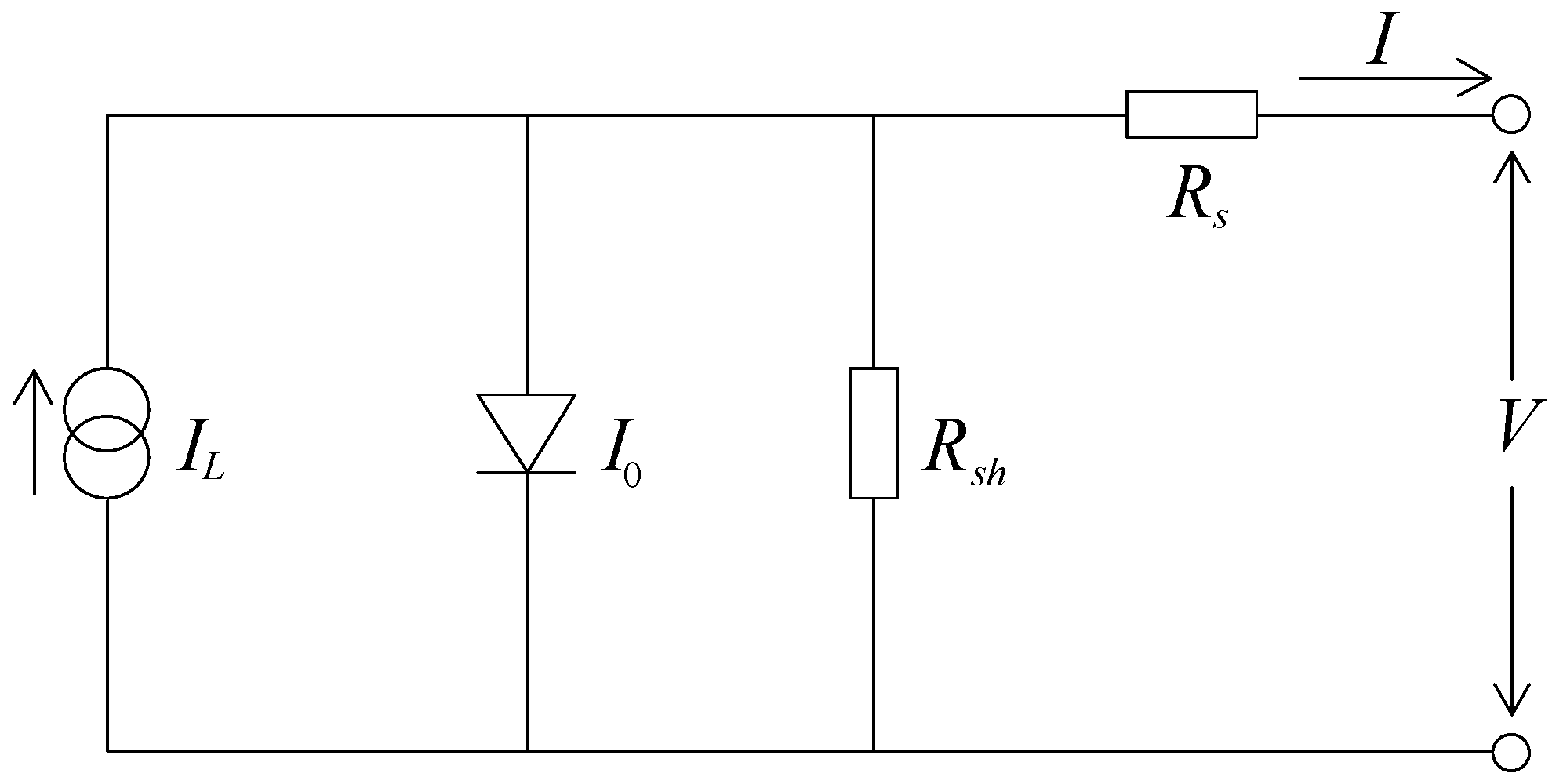
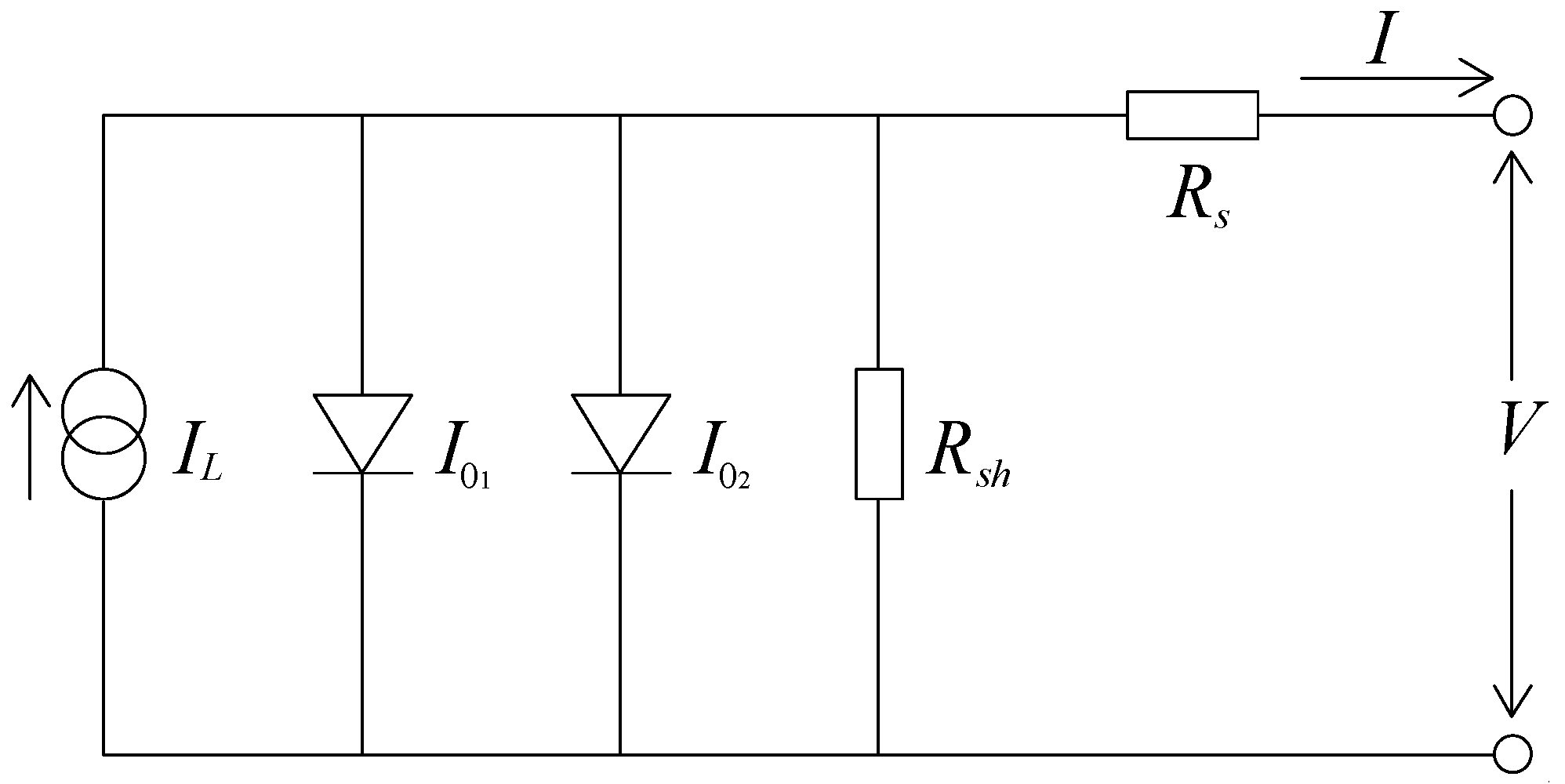
2] in order to represent the physical structure of a PV cell. As Wolf observed, the photocurrent in a PV cell is not generated by only one illuminated diode, but it is rather the global effect of the presence of a multitude of elementary flanked diodes that are uniformly distributed throughout the surface that separates the two slabs of the semiconductor junction. For this reason, a PV cell should be realistically approximated with a distributed constant electric circuit containing a multitude of elementary lumped components such as current generators, diodes and electrical resistances. Because such an equivalent circuit would be too complex to use, a simplified equivalent circuit was adopted. The circuit, which is depicted in Figure 1, contains only one pair of diodes with reverse saturation currents I01 and I02, a current generator and two resistors Rs and Rsh, which take account of dissipative effects and parasitic currents within the PV panel.
The second diode was added to consider the effect of the carrier recombination in the depletion region. The two-diode equivalent circuit of a PV module is described by the equation:
I = I L I 01 ( e V + I R s n 1 T 1 ) I 02 ( e V + I R s n 2 T 1 ) V + I R s R s h
where, following the traditional theory, the photocurrent IL depends on the solar irradiance, the diode saturation currents I01 and I02 are affected by the cell temperature, n1 = a1Ncsk/q and n2 = a2Ncsk/q are the diode quality factors, a1 and a2 are the diode shape factors, Ncs is the number of cells of the panel that are connected in series. The values of Rs, Rsh, I01 and I02 variously affect the I-V characteristic of the PV panel [
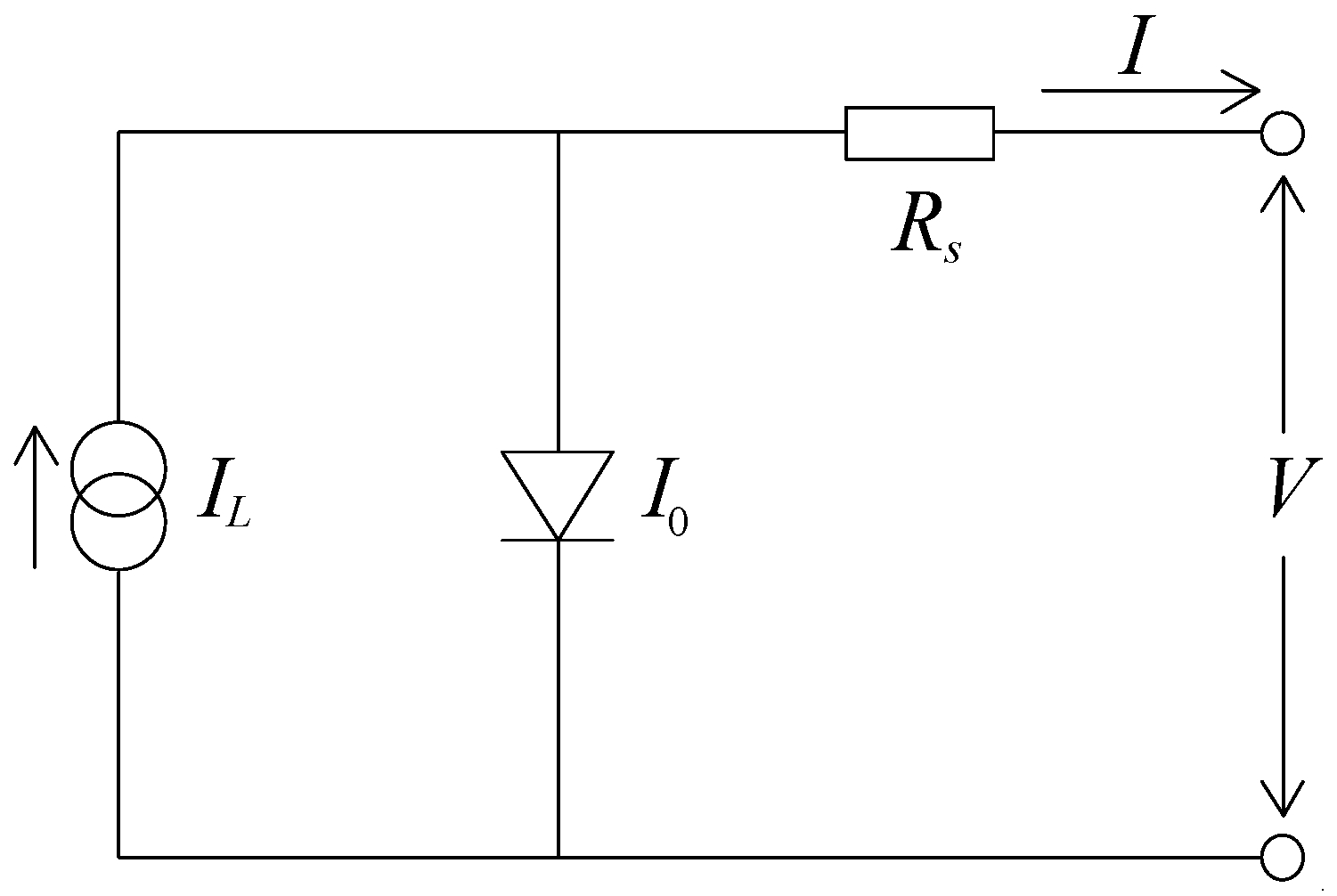
3]. Because the evaluation of the parameters contained in the two-diode equivalent circuit is a complex problem, the one-diode equivalent circuit, depicted in Figure 2, was also considered.
Many authors have proposed analytical procedures for determining the model parameters on the basis of the performance data usually provided by manufacturers [4,5,6,7,8,9,10,11,12,13,14,15,16,17,18,19,20,21,22,23,24,25,26,27,28,29,30,31,32,33,34,35,36,37,38,39,40,41,42,43,44,45,46,47,48]. The identification of the parameters contained in the diode-based equivalent circuits has been also tackled exploring the possibility of using different procedures such as Lambert W-function, evolutionary algorithms, Padè approximants, genetic algorithms, cluster analysis, artificial neural networks, harmony search-based algorithms, small perturbations around the operating point and reduced forms [49,50,51,52,53,54,55,56,57,58,59,60,61,62,63]. Other authors have investigated some simplified versions of the one-diode equivalent circuit in order to obtain an adequate representation of the PV panel characteristics by means of a reduced number of model parameters. A large amount of simplified one-diode models, obtained by changing the used set of performance data, the adopted hypotheses and the analytical procedures for evaluating the model parameters, have been presented [64,65,66,67,68,69,70,71,72].
The selection of the model fit for purpose may be a difficult task that should carefully consider both the strong points and weaknesses of the examined method. Besides the achievable precision, each model has a different usability, as it needs specific performance data, which may be not available or difficult to extract from the available datasheets. The model also presents computation difficulties, which may require the use of mathematical tools ranging from simple algorithms to complex methods implemented in dedicated computational software. The usability is a qualitative parameter, whereas the accuracy achievable by a model requires a quantitative assessment. In order to select the simplified one-diode model which represents the best compromise between analytical complexity and expected accuracy, it is necessary to perform a complex synthesis of both qualitative and quantitative features. The criterion proposed in this paper, which is used to rate the performances of some of the most famous simplified one-diode models, can help researchers and designers, working in the area of photovoltaic systems, to select the model fit for purpose.
The paper is organised along the lines of a previous study regarding the one-diode models for PV modules [1]. The criterion adopts a three-level rating scale that considers the ease of finding the data used by the analytical procedure, the simplicity of the mathematical tools needed to perform calculations and the accuracy achieved in calculating the current and power. Section 2 presents the simplified one-diode model and the effects of the series resistance on the shape of the I-V curves; Section 3 lists chronologically the most famous simplified one-diode equivalent circuits along with the used performance data, the required mathematical tools and the operative steps to obtain the model parameters. In Section 4, the accuracy of the tested simplified one-diode models is evaluated by calculating the I-V characteristics of some PV modules and comparing them with the performance curves issued by manufacturers. A criterion for rating the usability and accuracy of the analysed one-diode models is presented in Section 5. The minute descriptions of the mathematical procedures used to get the explicit or implicit expressions necessary to calculate the model parameters are listed in the Appendix A; such a review also contains the sequence of operative steps to easily calculate the model parameters.

2. The Simplified One-Diode Equivalent Circuit

The one-diode model depicted in Figure 2 is described by the well-known equation:
I = I L I 0 ( e V + I R s n T 1 ) V + I R s R s h
where diode quality factor n = aNcsk/q and a is the diode shape factor. Despite its simplicity, the one-diode model adequately reproduces the I-V characteristic at standard rating conditions (SRC)—irradiance Gref = 1000 W/m2, cell temperature Tref = 25 °C and average solar spectrum at AM 1.5—of most of the modern and efficient crystalline PV modules. Because of their small series resistance and great shunt resistance, crystalline PV modules show a good fill factor and, consequently, an I-V characteristic with a very sharp bend. The model is based on parameters IL, I0, n, Rs and Rsh whose calculation generally requires the solution of an equation system containing five independent relations obtained from Equation (2) or from its derivative. The mathematical difficulties encountered in the simultaneous solution of the involved implicit transcendent equations have suggested solving the problem by introducing some simplifications in the one-diode equivalent model. The four-parameter model depicted in Figure 3, in which resistance Rsh is set equal to infinity, has been often proposed.
The four-parameter model is governed by the following equation:
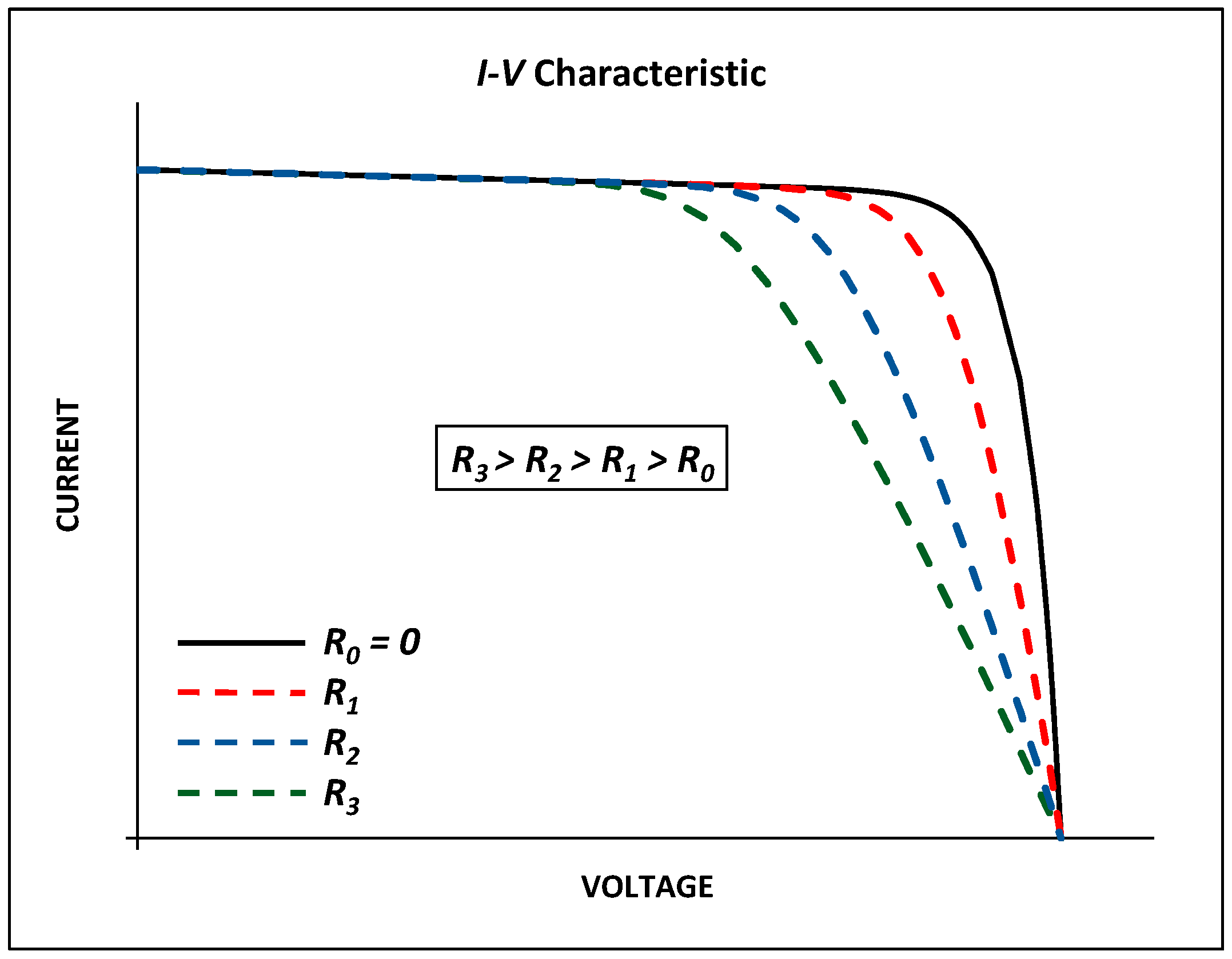
I = I L I 0 ( e V + I R s n T 1 )
As shown in Figure 4, series resistance Rs impacts the shape of the I-V characteristic close and beyond the MPP, which is approximately set on the “knee” of the curve.
At a constant value of the solar irradiance, if the series resistance is lowered, the internal dissipation of energy is reduced and the panel becomes more efficient; the MPP will slide towards right and the “knee” will be sharper because the value of the open circuit voltage is not affected by the series resistance. Conversely, smoother curves and greater values of Rs characterize the PV cells that are made with more energy dissipative materials and/or present higher electrical connection resistances. The analytical procedures proposed to calculate the four-parameter model generally require the following input data, which are usually available in the manufacturer datasheets:
  • open circuit voltage Voc,ref and short circuit current Isc,ref at the SRC;
  • voltage Vmp,ref and current Imp,ref at the MPP at the SRC;
  • open circuit voltage temperature coefficient μV,oc and short circuit current temperature coefficient μI,sc.
Sometimes, the number of series connected PV cells, or the derivative of the I-V curve at the MPP are also required. Because of the presence of current I in both terms of transcendent Equation (3), the solution of the four-equation system, which is necessary to calculate the model parameters, cannot be obtained by means of exact mathematical methods. To solve the problem, both approximate forms of the equations and numerical solving techniques have been used.

3. Usability of the Simplified One-Diode Models

Numerous procedures to calculate the parameters of the simplified one-diode model have been proposed. Some of these models were presented about 25 years ago. Nevertheless, they are still considered as effective and accurate as the most recent simplified one-diode models. Townsend [64] analysed several models of PV cells and panels and proposed a four-parameter model to be the most appropriate one for assessing the long-term performance of direct-coupled PV systems. In order to define the values of the model parameters, Townsend described three different procedures that in this paper are called Townsend n.1, Townsend n.2 and Townsend n.3, respectively. Other models were proposed by Duffie et al. [65], Xiao et al. [66], Ulapane et al. [67], Saloux et al. [68], Mahmoud et al. [69,70], Cristaldi et al. [71] and Averbukh et al. [72]. The model parameters are always evaluated by solving an equation system that represents the information related to the physical properties of the PV panels and/or geometrical conditions concerning the I-V characteristics.
The usability of a procedure may be significantly lowered by the difficulties encountered in using it. For this reason to assess the usability rating it is necessary to explore the complete sequence of operative steps that permit to calculate the model parameters. Sometimes the solution of the equation system is obtained adopting some simplifying hypotheses and iterative procedures. Some models evaluate the parameters on the basis of a similar set of information, but do not adopt the same simplifying hypotheses and/or use different relations to describe the dependence on the cell temperature and/or the solar irradiance. A synthetic description of the used information, simplifying hypotheses and solving techniques is contained in the paper and the analytical procedures to calculate the model parameters are minutely described in the Appendix A. Because the simplifying hypotheses are quite realistic, the values of the model parameters obtained by the approximate procedure may result almost equal to the values calculated without recourse to mathematical simplifications. Such an occurrence has been observed for some of the analysed models and consequently produces very similar I-V curves whose comparison may be considered trivial. Nevertheless, for the sake of completeness, the comparison of these models is also presented in this paper.

3.1. Townsend n.1 Model

The Townsend n.1 model [64] uses the following information:
(1)
short circuit point [I = Isc,ref; V = 0];
(2)
open circuit point [I = 0; V = Voc,ref];
(3)
MPP [I = Imp,ref; V = Vmp,ref];
(4)
derivative of power at the MPP [∂P/∂V = 0 at I = Imp,ref; V = Vmp,ref];
which are described by the four independent equations listed in the Appendix A. No simplifying hypothesis is assumed and the equation system is solved by means of the Newton-Raphson method.

3.2. Townsend n.2 Model

The Townsend n.2 model [64] is based on the same information of the Townsend n.1 model:
(1)
short circuit point [I = Isc,ref; V = 0];
(2)
open circuit point [I = 0; V = Voc,ref];
(3)
MPP [I = Imp,ref; V = Vmp,ref];
(4)
derivative of power at the MPP [∂P/∂V = 0 at I = Imp,ref; V = Vmp,ref].
The following hypotheses, which are usually verified for a PV module, are assumed:
e I s c , r e f R s n T r e f 1    e V o c , r e f n T r e f > > 1    e V m p , r e f n T r e f > > 1
and the model parameters can be calculated using the explicit equations described in the Appendix A.

3.3. Townsend n.3 Model

For the Townsend n.3 model [64] the following information is used:
(1)
short circuit point [I = Isc,ref; V = 0];
(2)
open circuit point [I = 0; V = Voc,ref];
(3)
MPP [I = Imp,ref; V = Vmp,ref];
(4)
derivative of voltage at the open circuit point [∂Voc/∂T = μV,oc at G = 1000 W/m2].
The same hypotheses of Equation (4) are assumed. Due to the presence of implicit forms, the equation system is solved with the iterative procedure described in the Appendix A.

3.4. Duffie and Beckman Model

The Duffie and Beckman model [65] is based on the same information used by the Townsend n.3 model:
(1)
short circuit point [I = Isc,ref; V = 0];
(2)
open circuit point [I = 0; V = Voc,ref];
(3)
MPP [I = Imp,ref; V = Vmp,ref];
(4)
derivative of voltage at the open circuit point [∂Voc/∂T = μV,oc at G = 1000 W/m2].
Due to the adoption of the hypotheses described in Equation (4), the model does not require any iterative procedure and parameters IL,ref, I0,ref, Rs and n can be calculated with the explicit equations listed in the Appendix A.

3.5. Xiao, Dunford and Capel Model

Xiao et al. [66] presented a four-parameter model whose parameters are calculated on the basis of the following information:
(1)
short circuit point [I = Isc,ref; V = 0];
(2)
open circuit point [I = 0; V = Voc,ref];
(3)
MPP [I = Imp,ref; V = Vmp,ref];
(4)
derivative of power at the MPP [∂P/∂V = 0 at I = Imp,ref; V = Vmp,ref].
Assuming the following hypothesis:
e I s c , r e f R s n T r e f 1
parameters IL,ref, I0,ref, n and Rs can be calculated with the iterative procedure described in the Appendix A.

3.6. Ulapane, Dhanapala, Wickramasinghe, Abeyratne, Rathnayake and Binduhewa Model

The model proposed by Ulapane et al. [67] uses the same information and hypothesis adopted by Xiao et al.
(1)
short circuit point [I = Isc,ref; V = 0];
(2)
open circuit point [I = 0; V = Voc,ref];
(3)
MPP [I = Imp,ref; V = Vmp,ref];
(4)
derivative of power at the MPP [∂P/∂V = 0 at I = Imp,ref; V = Vmp,ref].
The model parameters are calculated with the iterative procedure described in the Appendix A. A different approach is used to describe the physical behaviour of the PV panel for conditions far from the SRC.

3.7. Saloux, Teyssedou and Sorin Model

A three-parameter model, in which resistance Rs is set equal to zero, was proposed by Saloux at al. [68]. The model uses the following simplified analytical equation:
I = I L I 0 ( e V n T 1 )
The model parameters are calculated imposing that the following points belong to the I-V curve:
(1)
short circuit point [I = Isc,ref; V = 0];
(2)
open circuit point [I = 0; V = Voc,ref];
(3)
MPP [I = Imp,ref; V = Vmp,ref].
Assuming the following hypotheses:
e V o c , r e f n T r e f > > 1    e V m p , r e f n T r e f > > 1
the parameters of the model can be easily calculated with the explicit equations listed in the Appendix A.

3.8. Mahmoud, Xiao and Zeineldin n.1 Model

Mahmoud et al. [69] presented a three-parameter model based on Equation (6) whose parameters were calculated using the same information adopted by Saloux et al.
(1)
short circuit point [I = Isc,ref; V = 0];
(2)
open circuit point [I = 0; V = Voc,ref];
(3)
MPP [I = Imp,ref; V = Vmp,ref].
Numerical methods are used to solve the equations listed in the Appendix A. A different approach is adopted to describe the physical behaviour of the PV panel for conditions far from the SRC.

3.9. Cristaldi, Faifer, Rossi and Toscani Model

Cristaldi et al. [71] proposed a four-parameter model based on the following information:
(1)
short circuit point [I = Isc,ref; V = 0];
(2)
open circuit point [I = 0; V = Voc,ref];
(3)
MPP [I = Imp,ref; V = Vmp,ref];
(4)
derivative of power at the MPP [∂P/∂I = 0 at I = Imp,ref; V = Vmp,ref].
The following hypotheses are adopted:
e I s c , r e f R s n T r e f 1    e V o c , r e f n T r e f > > 1    e V o c , r e f n T r e f 0
and the model parameters are calculated by means of the analytical procedure based on the explicit equations listed in the Appendix A.

3.10. Averbukh, Lineykin and Kuperman Model

The model proposed by Averbukh et al. [72] uses on the same information used by Cristaldi et al.
(1)
short circuit point [I = Isc,ref; V = 0];
(2)
open circuit point [I = 0; V = Voc,ref];
(3)
MPP [I = Imp,ref; V = Vmp,ref];
(4)
derivative of power at the MPP [∂P/∂I = 0 at I = Imp,ref; V = Vmp,ref].
Instead of using Equation (3), the following equivalent expression is adopted:
V = n T ln ( I L I I 0 + 1 ) I R s
The equations listed in the Appendix A, which describe the short circuit, open circuit, maximum power points and the derivative of power at the MPP, are normalized using six per-unit dimensionless parameters and solved by means of a modern dedicate software.

3.11. Mahmoud, Xiao and Zeineldin n.2 Model

Mahmoud et al. [70] presented a procedure to automatically transform the five-parameter model into a four-parameter model, in which only the series resistance, or only the shunt resistance, is present. The equivalent circuit representation depends on the physical properties of the simulated PV panel. The model is based on the same information used by Cristaldi et al. and Averbukh et al.
(1)
short circuit point [I = Isc,ref; V = 0];
(2)
open circuit point [I = 0; V = Voc,ref];
(3)
MPP [I = Imp,ref; V = Vmp,ref];
(4)
derivative of power at the MPP [∂P/∂I = 0 at I = Imp,ref; V = Vmp,ref];
and assumes the following hypotheses:
e I s c , r e f R s n T r e f 1    I s c , r e f R s R s h 0    R s ( I 0 n T r e f e V m p , r e f + I m p , r e f R s n T r e f + 1 R s h ) < < 1
In order to state the equivalent circuit representation and calculate the model parameters, the procedure described in the Appendix A is adopted.

3.12. Summary of the Information Used by the Models

In order to better appreciate the analogies and differences between the various models, the used information, hypotheses and solving tools are summarised in Table 1.
It can be observed that the same information is often shared among different models. For this reason one may suppose that these models should be quite similar and yield the same results. Actually, because different simplifying hypotheses, solving techniques and relations to evaluate the PV panel performance curves at conditions different from SRC are adopted, each model has a particular capability to reproduce the I-V characteristics by means of mathematical approaches, which can be very simple or require the implementation of iterative routines and the use of specific mathematical methods and computer software.

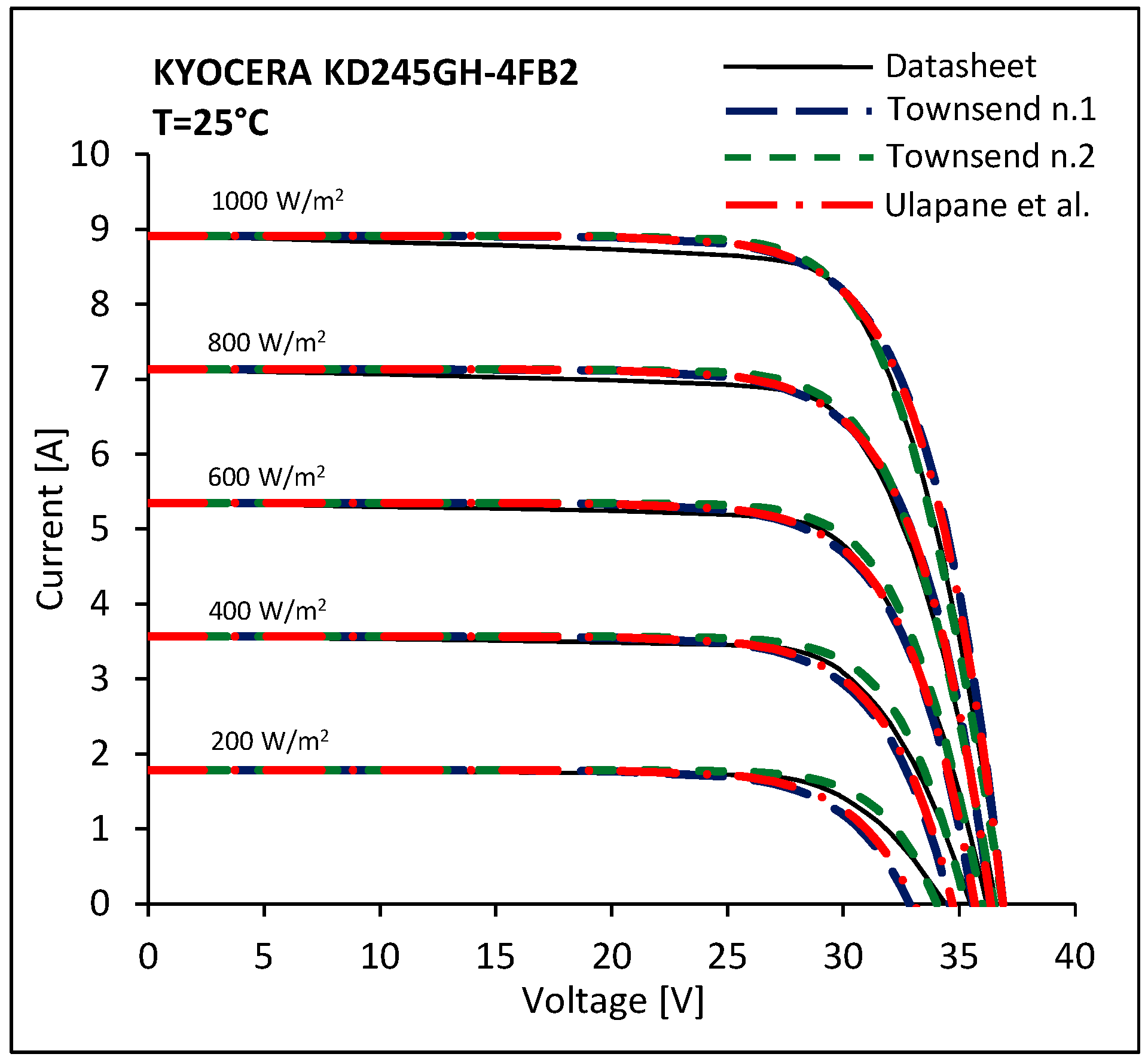
4. Accuracy of the Simplified One-Diode Models

With the aim of verifying the accuracy of the analysed procedures, a comparison between the simplified one-diode models was made using the I-V characteristics extracted from the manufacturer datasheets. For the sake of brevity only two PV modules, based on different technologies, were considered. Obviously, even using a greater number of PV modules, the comparison would never be exhaustive because the results are strongly affected by the particular shape of the considered I-V characteristics. Moreover, the purpose of this paper is not ranking the best or the worst among the analysed models, but only defining the range of predictable precision in order to calibrate the criterion. The performance data of the simulated PV modules are listed in Table 2.
Considering both the constant solar irradiance and the constant cell temperature curves, numerous points were extracted from the I-V characteristics issued by the manufacturers in order to get a reliable comparison between the calculated and the measured data. Table 3 and Table 4 list the values of the parameters evaluated with the analysed models.
For the analysed PV modules, the procedure proposed by the Mahmoud et al. n.2 model always generated an equivalent circuit representation in which only the series resistance is present. The values of Table 3 and Table 4 were used to calculate the I-V characteristics of the selected PV panels. The Townsend n.3 model was not considered because it perfectly corresponds to the Duffie et al. model. The Cristaldi et al. model was not taken into account because the I-V curves calculated with the model perfectly overlap the characteristics obtained from the Ulapane et al. model for all values of solar irradiance and cell temperature. Actually, the results are numerically indistinguishable because the only difference, which should make the Cristaldi et al. model a bit more imprecise, is due to the last two hypotheses described in Equation (8), which are thoroughly confirmed by real PV modules. In
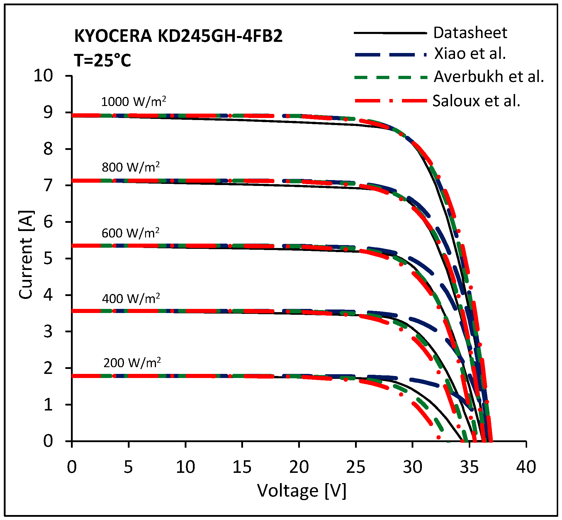
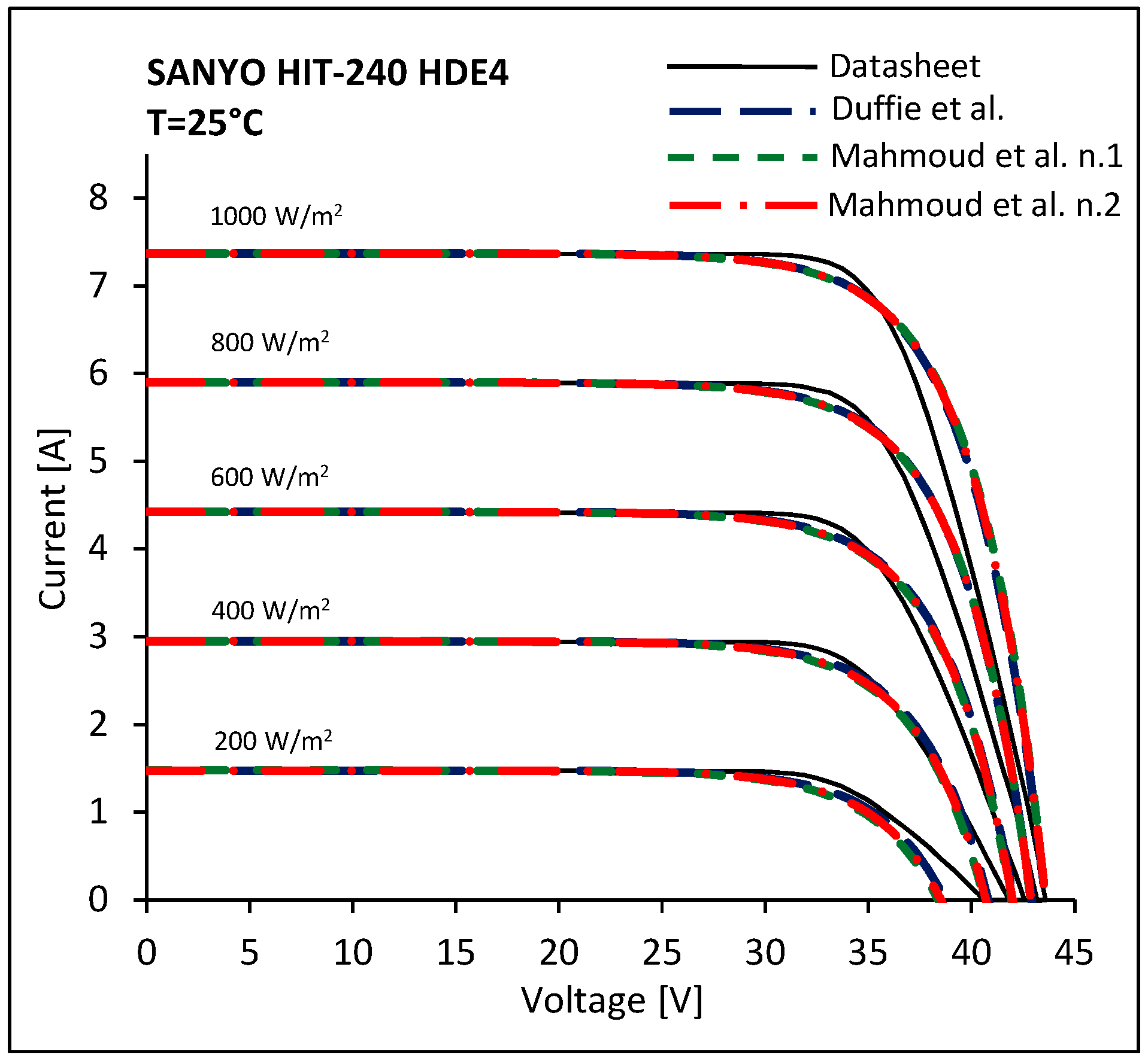
 Figure 5, Figure 6, Figure 7, Figure 8, Figure 9 and Figure 10 the I-V curves, evaluated at 
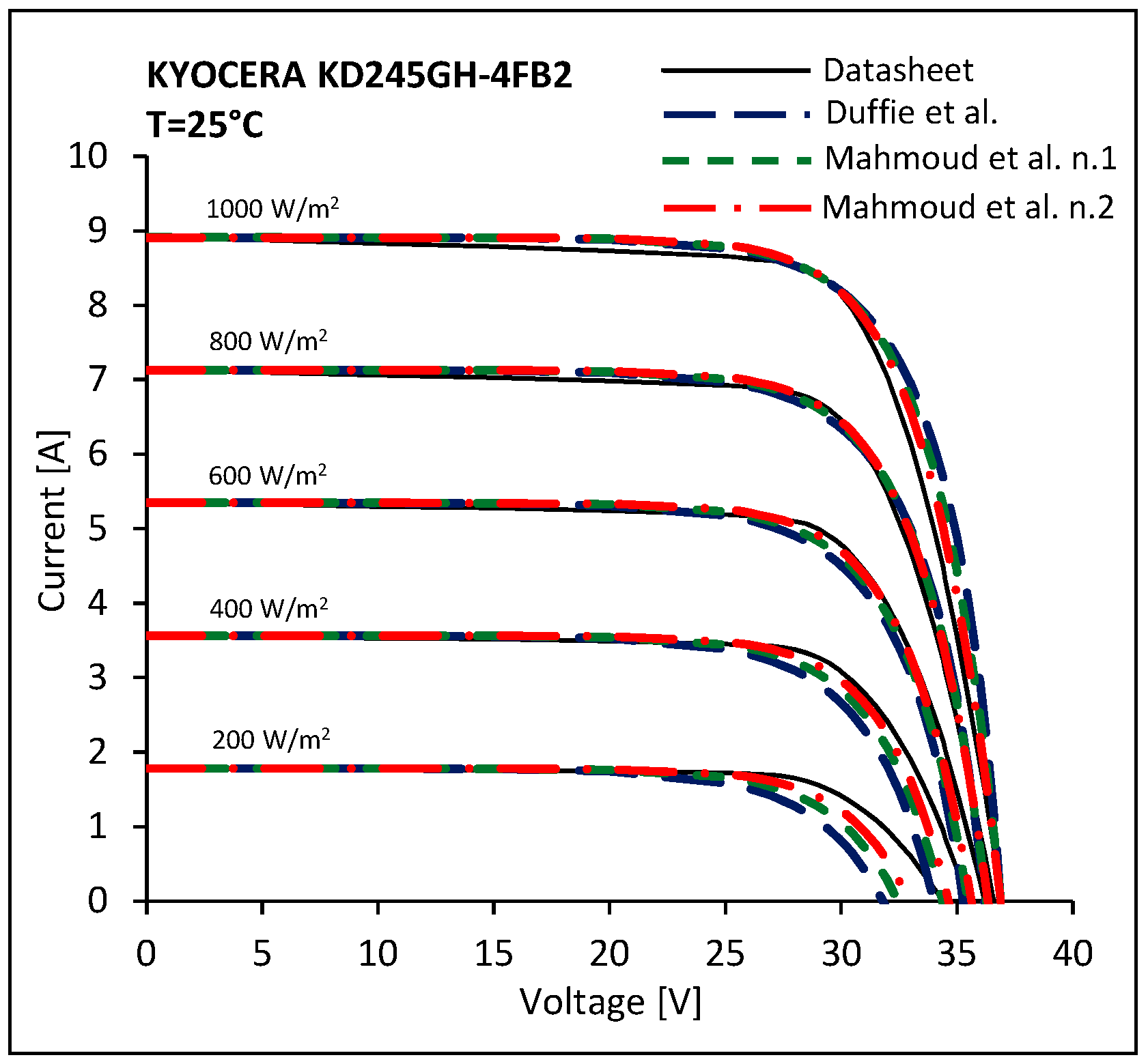
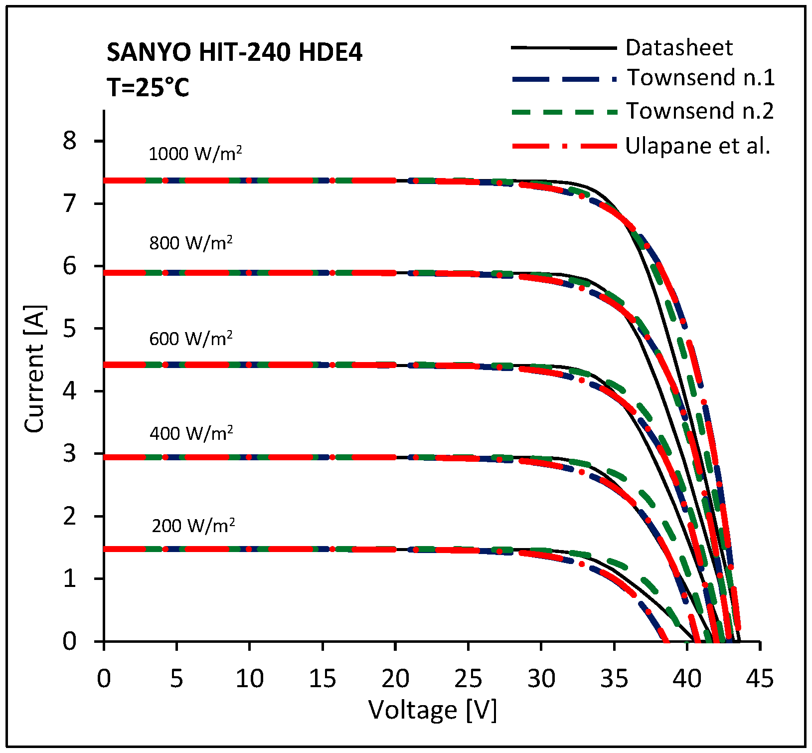
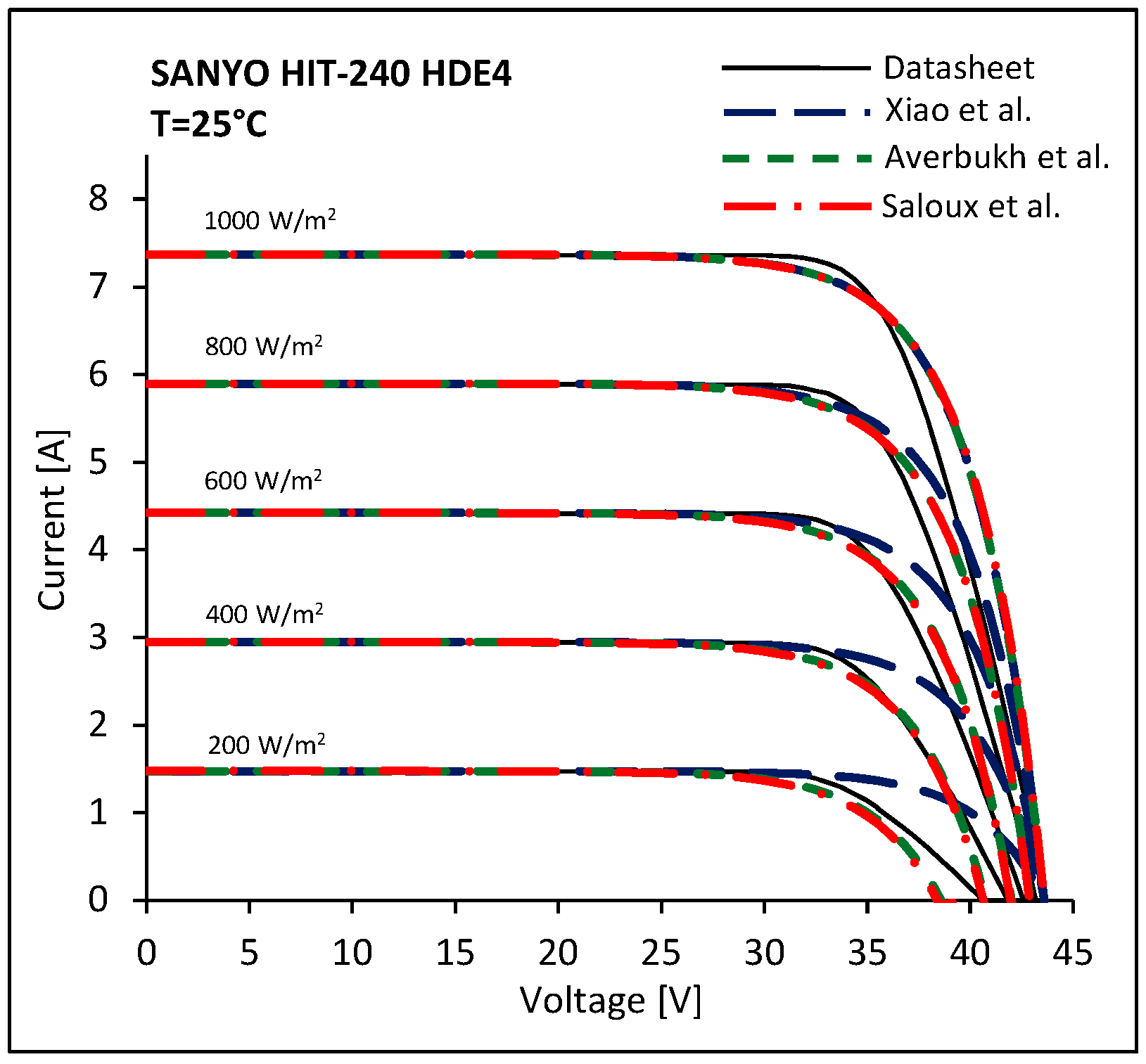
T = 25 °C, are compared with the characteristics issued by manufacturers.
Because the Xiao et al. the Ulapane et al. and the Averbukh et al. models are based on the same information, it is not surprising that the I-V curves at the SRC result quite similar. An analogous observation is valid for the Saloux et al. and the Mahmoud et al. n.1 models. Conversely, significant differences are expected for values of solar irradiance and cell temperature different from the SRC.
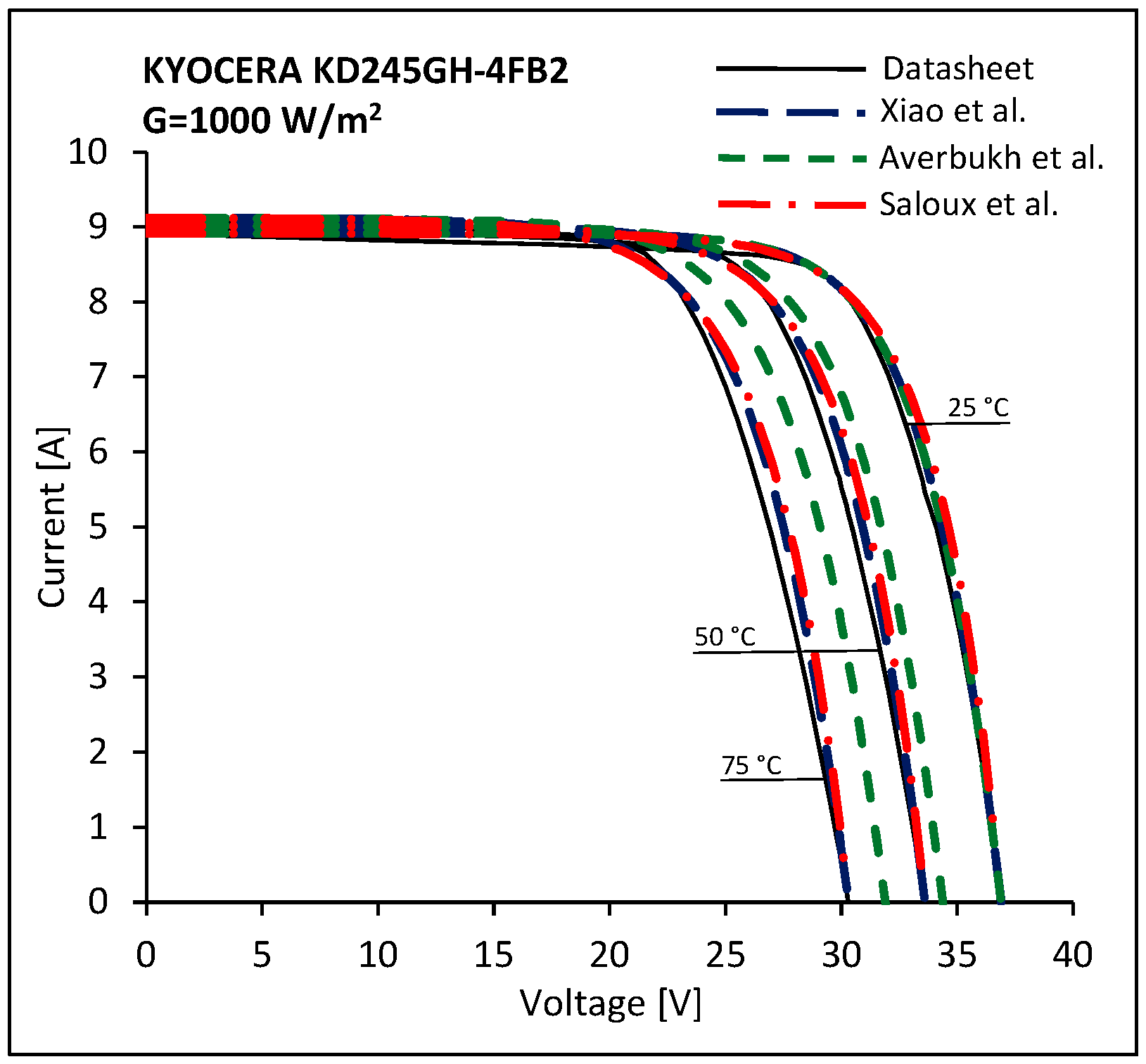
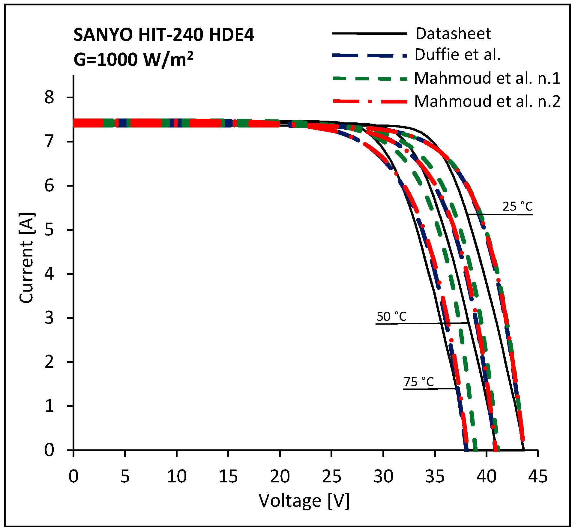
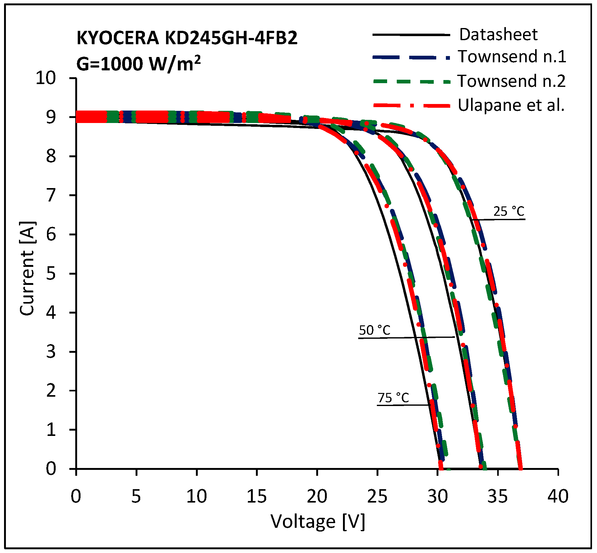
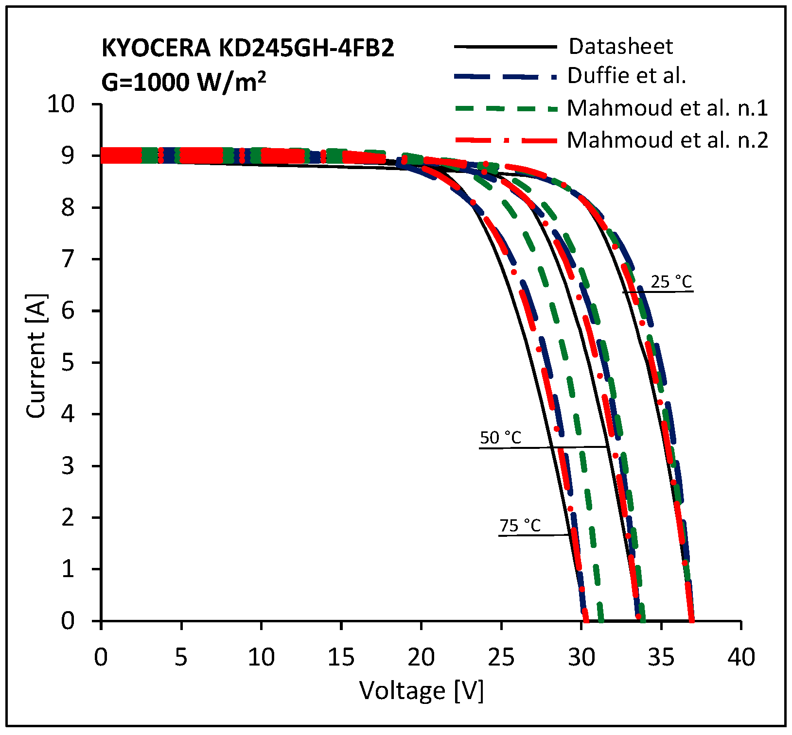
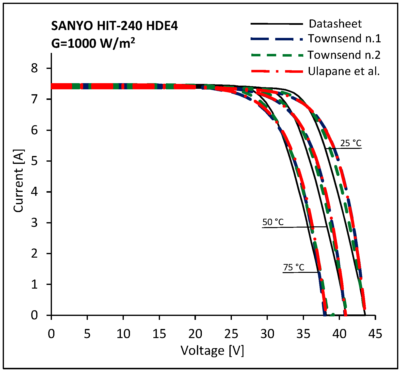
 Figure 11, Figure 12, Figure 13, Figure 14, Figure 15 and Figure 16 depict the I-V curves evaluated at G = 1000 W/m2 and the characteristics issued by manufacturers.
Observing Figure 5, Figure 6, Figure 7, Figure 8, Figure 9, Figure 10, Figure 11, Figure 12, Figure 13, Figure 14, Figure 15 and Figure 16 it can be generally deduced that all models result less accurate for voltage values greater than the MPP voltage. Moreover, it can be also noted that the simplified one-diode models are more precise if they are used to evaluate the I-V characteristics of the Kyocera PV panel. This occurrence may be due to the different shape of the I-V curves used to compare the analysed models. Actually, the I-V characteristics of the Sanyo module generally show sharper “knees” close to the MPP, probably due to the used heterojunction with intrinsic thin layer (HIT) technology. Moreover, it can be observed that models that use similar values of the parameters listed in Table 2 and Table 3 yield different I-V curves for values of the solar irradiance and the cell temperature far from the SRC; this condition is obviously due to the different approaches adopted to describe the effects of the solar irradiance and the cell temperature. In this respect, the models of Xiao et al. Mahmoud et al. n.1 and of Averbukh et al. seem to be less accurate. In order to quantify the accuracy of the analysed models, the mean absolute difference (MAD) for current and power was calculated using the following expressions:
MAD ( I ) = 1 N   j = 1 N | I c a l c , j I i s s , j |
MAD ( P ) = 1 N   j = 1 N | V i s s , j I c a l c , j V i s s , j I i s s , j |
in which Viss,j and Iiss,j are the voltage and current of the j-th point extracted from the I-V characteristics issued by manufacturers, Icalc,j is the value of the current calculated in correspondence of Viss,j and N is the number of extracted points. Moreover, in order to assess the range of dispersion of the results, also the maximum difference (MD) for current and power was evaluated using the following relations:
MD ( I ) = MAX [ I c a l c , j I i s s , j ]
MD ( P ) = MAX [ V i s s , j I c a l c , j V i s s , j I i s s , j ]
In Table 5 and Table 6, the percentage ratios of MAD(I) to the current at the issued MPP, and of MAD(P) to the rated maximum power, are listed.
In the last column the average values of the ratios of MAD(I) to the current at the issued MPP, and of MAD(P) to the rated maximum power, calculated for all I-V curves, are listed. For the Kyocera PV panel the smallest MAD(I)s range from 0.97% to 2.71% of the current at the MPP; the greatest MAD(I)s vary from 3.94% to 15.03%. The smallest MAD(I)s for the Sanyo PV module are in the range 0.92% to 3.18% of the current at the MPP; the greatest MAD(I)s range from 4.19% to 13.13%. The smallest MAD(P)s range from 0.97% to 2.49% of the rated maximum power for the Kyocera PV panel; the greatest MAD(P)s vary from 4.35% to 14.26%. For the Sanyo PV module the smallest MAD(P)s are in the range 0.93% to 3.05% of the rated maximum power; the greatest MAD(P)s vary from 4.64% to 13.25%. In Table 7 and Table 8 the values of MD(I) and MD(P) for the analysed panels, calculated considering the I-V curves at a constant cell temperature of 25 °C, are listed.
Considering the I-V curves at constant temperature of the Kyocera PV panel, the Townsend n.2 model seems to be the most accurate; the MD(I)s vary from 0.161 A to 0.259 A. The greatest current differences, which are contained in the range from 0.906 A to 1.379 A, are observed for the Duffie et al. and the Xiao et al. model. The smallest MD(I)s result for the Sanyo PV module by using the Townsend n.2, the Duffie et al. the Saloux et al. and the Mahmoud et al. n.1 models. These differences are in the range −0.356 to 0.632 A. The greatest inaccuracies derive from the Xiao et al., the Saloux et al. and the Mahmoud et al. n.1 models. For these models differences varying between 0.888 A and 1.403 A were calculated. Table 9 and Table 10 list the MD(I)s calculated for Kyocera KD245GH-4FB2 and Sanyo HIT-240 HDE4 PV panels at a constant solar irradiance of 1000 W/m2.
The smallest MD(I)s for the Kyocera PV module at constant solar irradiance are obtained by adopting the Townsend n.2 and the Ulapane et al. models. Such differences range from 0.206 A to 0.775 A. The greatest inaccuracies derive from the Duffie et al. and the Averbukh et al. models, for which differences varying between 1.332 A and 3.205 A are noted. The Townsend n.2 model seems to be the most accurate for the Sanyo PV panel; the MD(I)s vary from 0.531 A to 0.610 A. The greatest current differences, which are contained in the range from 1.221 A to 2.429 A, are provided by the Averbukh et al. the Saloux et al. and the Mahmoud et al. n.1 models. Table 11, Table 12, Table 13 and Table 14 show the effectiveness of the analysed models to predict the power generated by PV modules.
For the Kyocera PV panel, the smallest MD(P)s at constant cell temperature are again ascribed to the Townsend n.2 model that yields values varying from −5.84 W to 8.41 W. The greatest MD(P)s, which occur with the Xiao et al. and the Duffie et al. models, are in the range 32.15 W to 48.28 W. For the Sanyo PV module, the smallest MD(P)s at constant temperature, which vary from −14.46 W to 24.90 W, are obtained by means of the Townsend n.2, the Duffie et al. the Saloux et al. and the Mahmoud et al. n.1 models. The Xiao et al., the Saloux et al. and the Mahmoud et al. n.1 models yield the greatest inaccuracies, which vary from 35.80 W to 57.83 W.
Considering the MD(P)s at constant solar irradiance, the smallest values for the Kyocera PV panel are obtained by means of the Townsend n.2, the Xiao et al. and the Ulapane et al. models. The differences range −5.84 W to 20.76 W. The greatest inaccuracies derive from the Duffie et al. and the Averbukh et al. models. Differences, varying between 46.61 W and 97.01 W, were calculated. Townsend n.2 model yields the smallest MD(P)s for the Sanyo PV module, which are in the range from 19.19 W to 24.26 W. The greatest values are obtained with the Averbukh et al., the Saloux et al. and the Mahmoud et al. n.1 models. Such differences vary from 49.94 W to 92.72 W.

5. Rating of the Usability and Accuracy of the Simplified One-Diode Models

In order to rate the usability and accuracy of the analysed models, the same approach used in [1] was adopted. The rating criterion is based on a three-level rating scale that takes into consideration the following features:
  • the ease of finding the performance data used by the analytical procedure;
  • the simplicity of the mathematical tools needed to perform calculations;
  • the accuracy achieved in calculating the current and power of the analysed PV modules.
The ease of finding the input data is assumed:
  • high, when only tabular data are required (short circuit current, open circuit voltage, MPP current and voltage);
  • medium, when the data have to be extracted by reading the I-V characteristics (open circuit voltage at conditions different from the SRC);
  • low, when the derivative of the I-V curves are required.
The simplicity of the used mathematical tools is considered:
  • high, if only simple calculations are necessary;
  • medium, if an iterative procedure, which not necessarily requires dedicated computational software, is used;
  • low, when the analytical procedure requires the use of numerical solvers or complex mathematical methods usually implemented in dedicated computational software.
Table 15 lists the average ratios of MAD(I) to the rated current at the MPP, and of MAD(P) to the rated maximum power, extracted from Table 5 and Table 6.
It can be observed that the global accuracy listed in Table 15, which is calculated averaging the accuracies evaluated for the Kyocera and Sanyo PV panels, ranges from 2.34% to 4.68%. Such range of variation was divided in three equal intervals, which were used to qualitatively describe the accuracy of the analysed models:
  • high, for values of the mean difference in the subrange 2.34% to 3.12%;
  • medium, for values of the mean difference in the subrange 3.12% to 3.90%;
  • low, for values of the mean difference in the subrange 3.90% to 4.68%.
Table 16 lists the rating of the ease of finding data, simplicity of mathematical tools, and accuracy in calculating the current and power, based on the three-level rating scale previously described.
Excepting the Duffie et al. model, only data that are easy to be found are required by the models. Some models, such as Xiao et al., Mahmoud et al. n.1 and Averbukh et al. reach a small accuracy and present some mathematical difficulties. Other models such as the Townsend n.1 model and the Ulapane et al. model are more accurate. The Townsend n.2 model, Saloux et al. model and Mahmoud et al. n.2 model, which have high ratings for both the usability and accuracy, may be considered the best option among the simplified one-diode models.
In order to assess the suitability of using simplified one-diode models, it would be interesting to make a comparison with the performances of the best known one-diode models, when they are used to calculate the I-V characteristics of the same PV panels. Table 17 lists the usability and accuracy ratings of the one-diode models described in [1] along with the ones of the simplified one-diode models analysed in the present paper. To make a consistent comparison, the accuracy was rated considering the smallest and the greatest mean differences calculated for both the one-diode models and the simplified one-diode models. According to such extreme values, the following accuracy subranges were defined:
  • high, for values of the mean difference in the subrange 0.53% to 1.91%;
  • medium, for values of the mean difference in the subrange 1.91% to 3.30%;
  • low, for values of the mean difference in the subrange 3.30% to 4.68%.
The choice of the best model requires a wise compromise between usability and accuracy because no model achieves the highest ratings for all the considered features. In selecting a model one may prefer the usability to the accuracy, the accuracy to the usability, or try to find an acceptable balance between such features. As it was predictable, the models that reach a great accuracy require data more difficult to be found; adversely, the models based on data that can be easily read on the issued datasheets are generally less accurate. The best ratings are obtained by the Orioli et al. model, the Townsend n.2 model, the Saloux et al. model and the Mahmoud et al. n.2 model. The Orioli et al. model reaches a high precision although it presents some mathematical difficulties; the Townsend n.2 model, the Saloux et al. model and the Mahmoud et al. n.2 model are less precise but the model parameters can be easily calculated.

6. Conclusions

The analytical procedures to calculate the parameters of the models based on the simplified one-diode equivalent circuit were described, along with the simplifying hypotheses adopted. The models were used to calculate the I-V curves at constant cell temperature and solar irradiance using the data extracted from the manufacturers’ datasheets for two different types of PV modules. The calculated I-V curves were compared with the issued I-V characteristics in order to test the accuracy achievable by means of the analysed models. The model accuracies were quantified through the maximum difference and the mean absolute difference between the calculated values of current and the numerous values of current extracted from the issued I-V characteristics; the maximum difference and the mean absolute difference for the generated power were also evaluated.
Depending on the used model and the considered I-V curve, the most effective simplified one-diode equivalent circuits yielded for the poly-crystalline Kyocera KD245GH-4FB2 PV panel values of the current difference that averagely vary between 0.97% and 2.71% of the current at the MPP. The values of the power difference averagely ranged 0.97% to 2.49% of the rated maximum power. Smaller accuracies were generally observed for the Sanyo HIT-240 HDE4 PV module. The current differences averagely range 1.05% to 3.18% of the current at the MPP. The power accuracies averagely vary between 0.93% and 3.05% of the rated maximum power. The accuracies of the less effective models averagely reached 15.03% of the current at the MMP and 14.26% of the rated maximum power for the Kyocera PV panel, whereas average differences of 13.13% of the current at the MMP and of 13.25% of the rated maximum power were observed for the Sanyo PV module.
No model achieves the highest ratings for all the considered features. On the basis of the obtained results, the Townsend n.2 model and the Ulapane et al. model may be on average considered the most effective among the simplified one diode analysed models. If the model selection is extended to all the one-diode based models, the best ratings are given to the Orioli et al. model, the Townsend n.2 model, the Saloux et al. model and the Mahmoud et al. n.2 model. Actually it is not a trivial matter to identify the most accurate model because, depending on the type of PV panel and the particular I-V characteristic considered, the greatest accuracies are never obtained by means of the same model. Moreover, the aim of this paper is not to select the most effective model, but provide information useful to choose the analytical procedure that represents the best compromise between expected accuracy and mathematical complexity. Such a choice, which has to be wisely made aiming to the specific purpose, may be effectively supported by the results of the presented comparison.

Author Contributions

Aldo Orioli and Alessandra Di Gangi conceived and performed the criterion; Vincenzo Franzitta and Aldo Orioli carried out the analysis between the characteristics of the PV modules and the calculated current-voltage curves; Aldo Orioli and Alessandra Di Gangi wrote the paper.

Conflicts of Interest

The authors declare no conflicts of interest.

Appendix A

In this appendix the equations used by the various simplified one-diode models to describe the physical properties of PV panels are listed along with the analytical procedures adopted to get the explicit or implicit expressions necessary to calculate the equivalent model parameters.

Appendix A.1. Townsend n.1 Model

Townsend observed that, for the four-parameter equivalent circuit, it was not necessary to assign arbitrary values to any of the parameters because they could be univocally determined from the information usually provided by manufacturers at the SRC:
(1)
short circuit point [I = Isc,ref; V = 0];
(2)
open circuit point [I = 0; V = Voc,ref];
(3)
MPP [I = Imp,ref; V = Vmp,ref];
(4)
derivative of power at the MPP [∂P/∂V = 0 at I = Imp,ref; V = Vmp,ref].
Using the previous information, the following equations can be written:
  • I = Isc,ref and V = 0:
    I s c , r e f = I L , r e f I 0 , r e f ( e I s c , r e f R s n T r e f 1 )
  • I = 0 and V = Voc,ref:
    0 = I L , r e f I 0 , r e f ( e V o c , r e f n T r e f 1 )
  • I = Imp,ref and V = Vmp,ref:
    I m p , r e f = I L , r e f I 0 , r e f ( e V m p , r e f + I m p , r e f R s n T r e f 1 )
  • P/∂V = 0 at I = Imp,ref and V = Vmp,ref:
    P V | V = V m p , r e f I = I m p , r e f = ( V I ) V | V = V m p , r e f I = I m p , r e f = I m p , r e f + V m p , r e f I V | V = V m p , r e f I = I m p , r e f = 0
Because the partial derivative of the current is:
I V = I 0 , r e f n T r e f e V + I R s n T r e f 1 + R s I 0 , r e f n T r e f e V + I R s n T r e f
Equation (A4) is rewritten as:
I L , r e f + I 0 , r e f I 0 , r e f e V m p , r e f + I m p , r e f R s n T r e f ( 1 + 1 n T r e f 1 + R s I 0 , r e f n T r e f e V m p , r e f + I m p , r e f R s n T r e f ) = 0
To calculate the model parameters, the system of Equations (A1)–(A3) and (A6) was solved by Townsend by means of the Newton-Raphson method, which requires the direct calculation of the derivative of equations and the definition of initial values of parameters IL,ref, I0,ref, n and Rs within approximately an order of magnitude of the correct values, which is not an easy task. Unfortunately, the Newton-Raphson method, while rigorous, is fairly unstable and requires many computational steps to calculate the system parameters. In order to consider the effects of solar irradiance G and cell temperature T, Townsend proposed to use the following equations:
I L ( G , T ) = [ I s c , r e f + μ I , s c ( T T r e f ) ]   G G r e f
I 0 ( T ) = I 0 , r e f ( T T r e f ) 3 e N c s ε G n ( 1 T r e f     1 T )
in which εG, which is set 1.12 eV for Si and 1.35 eV for GaAs, is the bandgap energy of the material.

Appendix A.2. Townsend n.2 Model

The same information used by the Townsend n.1 model is considered. Assuming the following hypotheses:
e I s c , r e f R s n T r e f 1    e V o c , r e f n T r e f > > 1    e V m p , r e f n T r e f > > 1
Equations (A1)–(A3) can be rewritten as:
I s c , r e f = I L , r e f
0 = I L , r e f I 0 , r e f e V o c , r e f n T r e f
I m p , r e f = I L , r e f I 0 e V m p , r e f + I m p , r e f R s n T r e f = I s c , r e f ( 1 e V m p , r e f + I m p , r e f R s V o c , r e f n T r e f )
From Equations (A11) and (A12) the expressions of I0,ref and Rs are obtained:
I 0 , r e f = I s c , r e f e   V o c , r e f n T r e f
R s = n T r e f ln ( 1 I m p , r e f I s c , r e f ) + V o c , r e f V m p , r e f I m p , r e f
Because of Equation (A13), it is:
I = I L , r e f I 0 , r e f ( e V + I R s n T r e f 1 ) = I s c , r e f ( 1 e V + I R s V o c , r e f n T r e f + e   V o c , r e f n T r e f )
Equations (A5) and (A4) can be rewritten as:
I V = I s c , r e f n T r e f e V + I R s V o c , r e f n T r e f 1 + R s I s c , r e f n T r e f e V + I R s V o c , r e f n T r e f
I s c , r e f ( 1 e V m p , r e f + I m p , r e f R s V o c , r e f n T r e f ) V m p , r e f I s c , r e f n T r e f 1 + R s I s c , r e f n T r e f e V m p , r e f + I m p , r e f R s V o c , r e f n T r e f = 0
Moreover, considering that from Equations (A12) and (A14) it is:
I s c , r e f ( 1 e V m p , r e f + I m p , r e f R s V o c , r e f n T r e f ) = I s c , r e f I m p , r e f
I m p , r e f R s n T r e f = ln ( 1 I m p , r e f I s c , r e f ) + V o c , r e f V m p , r e f n T r e f
Equation (A17) can be solved in order to obtain the following expression:
n = 2 V m p , r e f V o c , r e f T r e f [ I m p , r e f I s c , r e f I m p , r e f + ln ( 1 I m p , r e f I s c , r e f ) ]
The values of IL,ref, n, I0,ref and Rs can be calculated by means of the explicit expressions (A10), (A20), (A13) and (A14). Townsend again suggested using of Equations (A7) and (A8) to describe the electrical behaviour of the analysed PV device far from the SRC.

Appendix A.3. Townsend n.3 Model

The following information is used:
(1)
short circuit point [I = Isc,ref; V = 0];
(2)
open circuit point [I = 0; V = Voc,ref];
(3)
MPP [I = Imp,ref; V = Vmp,ref];
(4)
derivative of the open circuit voltage [∂Voc/∂T = μV,oc at the SRC].
The same hypotheses of Equation (A9) are considered. Equations (A10) and (A13) are used to calculate IL,ref and I0,ref, whereas diode quality factor n is extracted from Equation (A12):
n = V m p , r e f + I m p , r e f R s V o c , r e f T r e f ln ( 1 I m p , r e f I s c , r e f )
Considering the fourth piece of information, an equation can be written by differentiating the expression of the open voltage obtained from Equations (A10) and (A11):
μ V , o c = V o c T | T = T r e f G = G r e f = T [ n T ln ( I s c I 0 ) ] T = T r e f G = G r e f
If Equations (A7) and (A8) are used to describe the dependence of Isc and I0 on the cell temperature, the following expression is obtained:
V o c T = n [ ln ( I s c I 0 ) + μ I , s c T I s c , r e f + μ I , s c ( T T r e f ) ( 3 + N c s ε G n T ) ]
that, at the SRC, becomes:
μ V , o c = V o c T | T = T r e f G = G r e f = n [ ln ( I s c , r e f I 0 , r e f ) + μ I , s c T r e f I s c , r e f ( 3 + N c s ε G n T r e f ) ]
It is evident that Equation (A24) can be calculated only if n and I0,ref are known. Moreover, diode reverse saturation current I0,ref in Equation (A13) depends on n and, in turn, the diode quality factor can be evaluated with Equation (A21) only if Rs is known. To calculate the model parameters with the above implicit equations, Townsend proposed an iterative procedure based on the following steps:
(1)
IL,ref is calculated by Equation (A10);
(2)
an initial value of Rs is assumed;
(3)
n is calculated by Equation (A21);
(4)
I0,ref is calculated by Equation (A13);
(5)
μV,oc is compared with the value calculated by Equation (A24);
(6)
the analytical procedure is concluded if the comparison is satisfied within a fixed accuracy; otherwise, a new value of Rs is assumed and the iterative procedure is repeated.
Townsend suggested using Equations (A7) and (A8) to describe the electrical behaviour of the analysed PV module far from the SRC. The Townsend n.3 model was also used by Chenni et al. [73] who partially issued the MS thesis of Eckstein [74].

Appendix A.4. Duffie and Beckman Model

The same information used by the Townsend n.3 model is used. Because the hypotheses of Equation (A9) are adopted, it is:
I L , r e f = I s c , r e f
I 0 , r e f = I s c , r e f e   V o c , r e f n T r e f
Equation (A14) is used to calculate Rs:
R s = n T r e f ln ( 1 I m p , r e f I s c , r e f ) V m p , r e f V o c , r e f I m p . r e f
If the following relation:
ln ( I s c , r e f I 0 , r e f ) = V o c , r e f n T r e f
which is derived from Equation (A26), is used in Equation (A24), it is possible to rewrite μV,oc in the form:
μ V , o c = V o c T | T = T r e f G = G r e f = V o c , r e f T r e f + n μ I , s c T r e f I s c , r e f ( 3 n + N c s ε G T r e f )
Parameter n is extracted from Equation (A29):
n = μ V , o c T r e f V o c , r e f + N c s ε G T r e f ( μ I , s c T r e f I s c , r e f 3 )
Parameters IL,ref, I0,ref, Rs and n can be calculated with Equations (A25)–(A27) and (A30). The effects of solar irradiance and cell temperature are evaluated using Equations (A7) and (A8). This method was adopted by Kou et al. [75] to estimate the long-term performance of direct-coupled PV pumping system. The model was also experimentally verified by Celik et al. [76].

Appendix A.5. Xiao, Dunford and Capel Model

The model uses the following information:
(1)
short circuit point [I = Isc,ref; V = 0];
(2)
open circuit point [I = 0; V = Voc,ref];
(3)
MPP [I = Imp,ref; V = Vmp,ref];
(4)
derivative of power at the MPP [∂P/∂V = 0 at I = Imp,ref; V = Vmp,ref].
Assuming the hypothesis:
e I s c , r e f R s n T r e f 1
from Equations (A1)–(A3) the following expressions of IL,ref, I0,ref and Rs can be extracted:
I L , r e f = I s c , r e f
I 0 , r e f = I s c , r e f e V o c , r e f n T r e f 1
R s = n T r e f ln [ ( 1 I m p , r e f I s c , r e f ) e V o c n T + I m p , r e f I s c , r e f ] V m p , r e f I m p , r e f
From Equation (A4), which describes the condition related to the derivative of the analytical power-voltage curve, the following equation can be obtained:
I V | V = V m p , r e f I = I m p , r e f + I m p , r e f V m p , r e f = 0
If Equation (A5) is used, Equation (A35) can be rewritten as:
I m p , r e f V m p , r e f I 0 , r e f n T r e f e V m p , r e f + I m p , r e f R s n T r e f 1 + R s I 0 , r e f n T r e f e V m p , r e f + I m p , r e f R s n T r e f = 0
Parameters IL,ref, I0,ref, n and Rs may be calculated with Equations (A32)–(A34) if parameter n, was known; such a parameter is also present in Equation (A36), which describes the condition related to the derivative of the analytical power-voltage curve. Because of the presence of implicit equations, the model parameters are calculated with the following iterative procedure:
(1)
IL,ref is calculated by Equation (A32);
(2)
an initial value of n is assumed;
(3)
I0,ref is calculated by Equation (A33);
(4)
Rs is calculated by Equation (A34);
(5)
Equation (A36) is calculated;
(6)
the analytical procedure is concluded if Equation (A36) is verified within a fixed accuracy; otherwise, a new value of n is assumed and the iterative procedure is repeated.
In order to take account of the effects of solar irradiance and cell temperature different from the SRC, photocurrent IL is calculated with Equation (A7), whereas reverse saturation current I0 is evaluated by means of the following equation, which is derived from Equation (A33):
I 0 ( G , T ) = [ I s c , r e f + μ I , s c ( T T r e f ) ]   G G r e f e V o c , r e f + μ V , o c ( T T r e f ) n T 1
where thermal coefficient μI,sc and μV,oc are used.

Appendix A.6. Ulapane, Dhanapala, Wickramasinghe, Abeyratne, Rathnayake and Binduhewa Model

Because the same information an hypothesis used by the Xiao et al. model are considered, currents IL,ref and I0,ref can be calculated with Equations (A32) and (A33). From the condition describing the MPP, the following expressions are obtained:
R s = n T r e f I m p , r e f ln ( I L , r e f I m p , r e f + I 0 , r e f I 0 , r e f ) V m p , r e f I m p , r e f
I 0 , r e f e V m p , r e f + I m p , r e f R s n T r e f = I L , r e f I m p , r e f + I 0 , r e f
Equation (A36), which refers to the derivative of the power in the MPP, can be rewritten in the following form:
n T r e f I m p , r e f + ( I m p , r e f R s V m p , r e f ) I 0 , r e f e V m p , r e f + I m p , r e f R s n T r e f V m p , r e f ( n T r e f + R s I 0 , r e f e V m p , r e f + I m p , r e f R s n T r e f ) = 0
If Equations (A38) and (A39) are used in the above equation, the following expression, which is equivalent to Equation (A40), is obtained:
n T r e f I m p , r e f + ( I L , r e f I m p , r e f + I 0 , r e f ) [ n T r e f ln ( I L , r e f I m p , r e f + I 0 , r e f I 0 , r e f ) 2 V m p , r e f ] = 0
The model parameters are calculated with the procedure summarized in the following steps:
(1)
IL,ref is calculated by Equation (A32);
(2)
the expression of I0,ref from Equation (A33) is substituted in Equation (A41);
(3)
n is calculated by solving Equation (A40) with the Newton-Raphson method;
(4)
I0,ref is calculated by Equation (A33);
(5)
Rs is calculated by Equation (A38).
For conditions different from the SRC, photocurrent IL(G,T) is calculated with Equation (A7), whereas the following relation is adopted for the reverse saturation current:
I 0 ( G , T ) = I L ( G , T ) e V o c ( G , T ) n T 1
For the open circuit voltage, the following expression:
V o c ( G , T ) = V o c , r e f + μ V , o c ( T T r e f ) + n T ln ( G G r e f )
proposed by Chenlo et al. [77], is used.

Appendix A.7. Saloux, Teyssedou and Sorin Model

The model uses the following information:
(1)
short circuit point [I = Isc,ref; V = 0];
(2)
open circuit point [I = 0; V = Voc,ref];
(3)
MPP [I = Imp,ref; V = Vmp,ref].
that permit to write the following equations obtained by Equation (6):
I s c , r e f = I L , r e f
0 = I L , r e f I 0 , r e f ( e V o c , r e f n T r e f 1 )
I m p , r e f = I L , r e f I 0 , r e f ( e V m p , r e f n T r e f 1 )
If it is assumed:
e V o c , r e f n T r e f > > 1    e V m p , r e f n T r e f > > 1
it is possible to extract I0,ref from Equation (A45):
I 0 , r e f = I s c , r e f e   V o c , r e f n T r e f
Equation (A48) can be substituted in Equation (A46) in order to write the following expression:
I m p , r e f = I L , r e f I L , r e f e V m p , r e f V o c , r e f n T r e f
from which parameter n is extracted:
n = V m p , r e f V o c , r e f T r e f ln ( 1 I m p , r e f I L , r e f )
the parameters of the model can be calculated with the following sequence of steps:
(1)
IL,ref is calculated by Equation (A44);
(2)
n is calculated by Equation (A50);
(3)
I0,ref is calculated by Equation (A48).
To take account of the effects of values of the solar irradiance and cell temperature different from the SRC, photocurrent IL and reverse saturation current I0 are calculated with Equations (A7), (A42) and (A43).

Appendix A.8. Mahmoud, Xiao and Zeineldin n.1 Model

The same information used by the Saloux et al. model is considered. Due to the use of Equation (6), currents IL,ref and I0,ref can be calculated with Equations (A32) and (A33). Equation (A33) is substituted in Equation (A46) to calculate parameter n:
I m p , r e f = I s c , r e f I s c , r e f e V o c , r e f n T r e f 1 ( e V m p , r e f n T r e f 1 )
The model parameters are calculated with the following procedure:
(1)
IL,ref is calculated by Equation (A32);
(2)
n is calculated by solving Equation (A51) by means of numerical methods;
(3)
I0,ref is calculated by Equation (A33).
In order to use the model for values of the solar irradiance and cell temperature different from the SRC, it is assumed that:
μ V , o c ( T T r e f ) = V o c ( G , T ) V o c ( G , T r e f )
Because in the open circuit point it is:
0 = I L ( G , T ) I 0 ( G , T ) [ e V o c ( G , T ) n T 1 ]
the following forms can be substituted in Equation (A52):
V o c ( G , T ) = n T ln [ I L ( G , T ) I 0 ( G , T ) + 1 ]
V o c ( G , T r e f ) = n T ln [ I L ( G , T r e f ) I 0 , r e f + 1 ]
Due to the above substitutions, and expressing IL(G,T) with Equation (A7), it is possible to extract I0(G,T) from Equation (A52):
I 0 ( G , T ) = e μ V , o c ( T T r e f ) n T [ I s c , r e f + μ I , s c ( T T r e f ) ] G G r e f ( I s c , r e f G I 0 , r e f G r e f + 1 ) T r e f T e μ V , o c ( T T r e f ) n T
Equations (A7) and (A56) are used in Equation (6) to calculate the I-V characteristics for any values of G and T.

Appendix A.9. Cristaldi, Faifer, Rossi and Toscani Model

The model uses the following information:
(1)
short circuit point [I = Isc,ref; V = 0];
(2)
open circuit point [I = 0; V = Voc,ref];
(3)
MPP [I = Imp,ref; V = Vmp,ref];
(4)
derivative of power at the MPP [∂P/∂I = 0 at I = Imp,ref; V = Vmp,ref].
The following hypotheses are also adopted:
e I s c , r e f R s n T r e f 1    e V o c , r e f n T r e f > > 1    e V o c , r e f n T r e f 0
From the information regarding the short circuit and open circuit points, Equations (A32) and (A13) can be obtained and used to write Equation (3) in the following form:
I = I L , r e f I 0 , r e f ( e V + I R s n T r e f 1 ) = I s c , r e f ( 1 e V + I R s V o c , r e f n T r e f + e   V o c , r e f n T r e f )
Considering the third hypothesis in Equation (A57), the following expression is obtained from Equation (A58):
V = V o c , r e f + n T r e f ln ( 1 I I s c , r e f ) I R s
Because of the conditions related to the MPP and the derivative of the power in the MPP, it is:
V m p , r e f = V o c , r e f + n T r e f ln ( 1 I m p , r e f I s c , r e f ) I m p , r e f R s
P I | V = V m p , r e f I = I m p , r e f = ( V I ) I | V = V m p , r e f I = I m p , r e f = I m p , r e f V I | V = V m p , r e f I = I m p , r e f + V m p , r e f = 0
Because I0,ref << IL,ref, the derivative of voltage is:
V I | = n T r e f I L , r e f I + I 0 , r e f R s n T r e f I s c , r e f I R s
and Equation (A61) can be rewritten in the following form:
( V I ) I | V = V m p , r e f I = I m p , r e f = V m p , r e f n T r e f I m p , r e f I s c , r e f I m p , r e f I m p , r e f R s = 0
Solving Equations (A60) and (A63), the following expressions are obtained:
n = ( 2 V m p , r e f V o c , r e f ) ( I s c , r e f I m p , r e f ) T r e f [ I m p , r e f + ( I s c , r e f I m p , r e f ) ln ( 1 I m p , r e f I s c , r e f ) ]
R s = V m p , r e f I m p , r e f 2 V m p , r e f V o c , r e f I m p , r e f + ( I s c , r e f I m p , r e f ) ln ( 1 I m p , r e f I s c , r e f )
The model parameters can be calculated with the following steps:
(1)
IL,ref is calculated by Equation (A32);
(2)
n is calculated by Equation (A54);
(3)
I0,ref is calculated by Equation (A13);
(4)
Rs is calculated by Equation (A65).
The effects due to values of the solar irradiance and cell temperature different from the SRC are considered by means of Equation (A7) and (A43).

Appendix A.10. Averbukh, Lineykin and Kuperman Model

The same information used by the Cristaldi et al. model is considered. Using Equation (9), the conditions regarding the short circuit, open circuit and maximum power points correspond to the equations:
0 = n T r e f ln ( I L , r e f I s c , r e f I 0 , r e f + 1 ) I s c , r e f R s
V o c , r e f = n T r e f ln ( I L , r e f I 0 , r e f + 1 )
V m p , r e f = n T r e f ln ( I L , r e f I m p , r e f I 0 , r e f + 1 ) I m p , r e f R s
The condition for the derivative of power at the MPP is described by Equation (A61). Because the partial derivative of the voltage is:
V I = n T r e f I L , r e f I + I 0 , r e f R s
Equation (A61) can be rewritten as:
n T r e f ln ( I L , r e f I m p , r e f I 0 , r e f + 1 ) ( n T r e f I L , r e f I m p , r e f + I 0 , r e f + 2 R s ) I m p , r e f = 0
Equations (A66), (A65), (A68) and (A70) are normalized using the following per-unit dimensionless parameters:
α = I 0 , r e f I L , r e f β = I L , r e f R s n T r e f v o c = V o c , r e f n T r e f χ s c = I s c , r e f I L , r e f v m = V m p , r e f n T r e f χ m = I m p , r e f I L , r e f
and solved by means of a modern dedicate software. The hypothesis in Equation (5) is again assumed and, consequently, it is IL,ref = Isc,ref. Parameters n, I0,ref and Rs are extracted from the calculated values of vm, α and β, respectively. In order to obtain the operational I-V curves for arbitrary conditions of solar irradiance and cell temperature, Equation (A7) is assumed. The following equation:
I 0 ( T ) = I 0 , r e f e N c s ε G n ( 1 T r e f     1 T )
is used to describe the reverse saturation current.

Appendix A.11. Mahmoud, Xiao and Zeineldin n.2 Model

The model is based on the same information used by Cristaldi et al. and Averbukh et al. Assuming for Equation (2) the hypotheses:
e I s c , r e f R s n T r e f 1    I s c , r e f R s R s h 0
the short circuit and open circuit conditions permit to write the following expressions:
I L , r e f = I s c , r e f
I 0 , r e f = I L , r e f V o c , r e f / R s h e V o c , r e f n T r e f 1
The condition on the MPP is expressed by the equation:
I m p , r e f = I L , r e f I 0 , r e f ( e V m p , r e f + I m p , r e f R s n T r e f 1 ) V m p , r e f + I m p , r e f R s R s h
For the five-parameter model the derivative of current at the MPP is:
I V | V = V m p , r e f I = I m p , r e f = I 0 n T r e f e V m p , r e f + I m p , r e f R s n T r e f + 1 R s h 1 + R s ( I 0 n T r e f e V m p , r e f + I m p , r e f R s n T r e f + 1 R s h )
If Equations (A74) and (A75) are substituted in Equations (A76) and (A4), which refers to the derivative of power at the MPP, and in Equation (A77) it is assumed that:
R s ( I 0 n T r e f e V m p , r e f + I m p , r e f R s n T r e f + 1 R s h ) < < 1
the following equations can be written:
0 = I s c , r e f I L , r e f V o c , r e f / R s h e V o c , r e f n T r e f 1 [ ( 1 + V m p , r e f n T r e f ) e V m p , r e f + I m p , r e f R s n T r e f 1 ] 2 V m p , r e f + I m p , r e f R s R s h
0 = [ I s c , r e f R s h V m p , r e f I m p , r e f ( R s + R s h ) I s c , r e f R s h V o c , r e f ] e V o c , r e f n T r e f + e V m p , r e f + I m p , r e f R s , r e f n T r e f [ V o c , r e f V m p , r e f I m p , r e f ( R s , r e f + R s h , r e f ) I s c , r e f R s h V o c , r e f ]
The five-parameter model is transformed into a four-parameter model, in which only the series resistance, or only the shunt resistance, is present by means of the following procedure:
(1)
IL,ref is calculated by Equation (A74);
(2)
it is set Rsh = ∞ (Rsh = 107);
(3)
Rs and n are calculated by simultaneously solving Equations (A79) and (A80);
(4)
if a solution for Rs and n, within a feasible region, is reached, then the model only contains Rs;
(5)
otherwise, it is set Rs = 0;
(6)
Rsh and n are calculated by simultaneously solving Equations (A79) and (A80);
(7)
I0,ref is calculated by Equation (A75).
To calculate the I-V characteristics for generic values of solar irradiance and cell temperature, photocurrent IL(G,T) are descripted by Equation (A7). For the reverse saturation current, the following equation is used:
I 0 ( G , T ) = G G r e f [ I L , r e f + μ I , s c ( T T r e f ) ] e | μ V , o c | ( T T r e f ) n T ( G G r e f I s c , r e f I 0 , r e f + 1 ) T r e f T e | μ V , o c | ( T T r e f ) n T

Nomenclature

a, a1, a2diode shape factors
Gsolar irradiance (W/m2)
Grefsolar irradiance at the SRC (1000 W/m2)
Icurrent generated by the panel (A)
Icalc,jcurrent of the j-th calculated point of the I-V characteristic (A)
Iiss,jcurrent of the j-th point extracted from the issued I-V characteristic (A)
ILphotocurrent (A)
IL,refphotocurrent (A) at the SRC (A)
Imp,refcurrent in the maximum power point at the SRC (A)
Iscshort circuit current of the panel (A)
Isc,refshort circuit current of the panel at the SRC (A)
I0, I01, I02diode saturation current (A)
I0,refdiode saturation current at the SRC (A)
kBoltzmann constant (J/K)
n, n1, n2diode quality factors (V/K)
Nnumber of points extracted from the issued I-V characteristic
Ncsnumber of cells connected in series
Ppower generated by the panel (W)
qelectron charge (C)
Rsseries resistance (Ω)
Rshshunt resistance (Ω)
Ttemperature of the PV cell (°K)
Treftemperature of the PV panel at the SRC (25 °C–298.15 °K)
Vvoltage generated by the PV panel (V)
Vocopen circuit voltage of the PV panel (V)
Voc,refopen circuit voltage of the PV panel at the SRC (V)
Viss,jvoltage of the j-th point extracted from the issued I-V characteristic (A)
Vmp,refvoltage in the maximum power point at the SRC (V)
VTvoltage in the maximum power point at the SRC (V)
εGbandgap energy of the material (eV)
μI,scthermal coefficient of the short circuit current (A/°C)
μV,octhermal coefficient of the open circuit voltage (V/°C)

References

  1. Orioli, A.; Di Gangi, A. A criterion for rating the usability and accuracy of the one-diode models for photovoltaic modules. Energies 2016, 9, 427. [Google Scholar] [CrossRef] [Green Version]
  2. Wolf, M.; Rauscenbach, H. Series Resistance Effects on Solar Cell Measurements. Adv. Energy Convers. 1963, 3, 455–479. [Google Scholar] [CrossRef]
  3. Markvart, T.; Costañer, L. Solar Cells: Materials, Manufacture and Operation; Elsevier: Oxford, UK, 2005. [Google Scholar]
  4. Chan, D.S.H.; Phang, J.C.H. Analytical methods for the extraction of solar-cell single- and double-diode model parameters from I-V characteristics. IEEE Trans. Electron Devices 1987, 34, 286–293. [Google Scholar] [CrossRef]
  5. Enebish, N.; Agchbayar, D.; Dorjkhand, S.; Baatar, D.; Ylemj, I. Numerical analysis of solar cell current-voltage characteristics. Sol. Energy Mater. Sol. Cells 1993, 29, 201–208. [Google Scholar] [CrossRef]
  6. Hovinen, A. Fitting of the solar cell IV-curve to the two diode model. Phys. Scr. 1994, T54, 175–176. [Google Scholar] [CrossRef]
  7. Garrido-Alzar, C.L. Algorithm for extraction of solar cell parameters from I-V curve using double exponential model. Renew. Energy 1997, 10, 125–128. [Google Scholar] [CrossRef]
  8. Zhao, R.; Xu, H.; Zhao, Z.; Zhang, S. A simplified double-exponential model of potovoltaic module in matlab™. In Proceedings of the IEEE International Conference on Energy and Environment Technology (ICEET ’09), Guilin, China, 16–18 October 2009; pp. 157–160.
  9. Yordanov, G.H.; Midtgård, O.M.; Saetre, T.O. Two-diode model revisited: Parameters extraction from semi-log plots of I-V data. In Proceedings of the 25th European Photovoltaic Solar Energy Conference and Exhibition/5th World Conference on Photovoltaic Energy Conversion, Valencia, Spain, 6–10 September 2010; pp. 4156–4163.
  10. Yordanov, G.H.; Midtgård, O.M.; Saetre, T.O. Extracting parameters from semi-log plots of polycrystalline silicon PV modules outdoor I-V data: Double-exponential model revisited. In Proceedings of the 35th IEEE Photovoltaic Specialists Conference (PVSC), Honolulu, HI, USA, 20–25 June 2010; pp. 2756–2761.
  11. Ishaque, K.; Salam, Z.; Taheri, H. Simple, fast and accurate two-diode model for photovoltaic modules. Sol. Energy Mater. Sol. Cells 2011, 95, 586–594. [Google Scholar] [CrossRef]
  12. Gupta, S.; Tiwari, H.; Fozdar, M.; Chandna, V. Development of a two diode model for photovoltaic modules suitable for use in simulation studies. In Proceedings of the 2012 Asia-Pacific Power and Energy Engineering Conference (APPEEC), Shanghai, China, 27–29 March 2012; pp. 1–4.
  13. Maoucha, A.; Djeffal, F.; Arar, D.; Lakhdar, N.; Bendib, T.; Abdi, M.A. An accurate organic solar cell parameters extraction approach based on the illuminated I-V characteristics for double diode modelling. In Proceedings of the 1st International Conference on renewable Energies and Vehicular Technology (REVET), Nabeul, Tunisia, 26–28 March 2012; pp. 74–77.
  14. Hejri, M.; Mokhtari, H.; Azizian, M.R.; Ghandhari, M.; Söder, L. On the parameter extraction of a five-parameter double-diode model of photovoltaic cells and modules. IEEE J. Photovolt. 2014, 4, 915–923. [Google Scholar] [CrossRef]
  15. Babu, B.C.; Gurjar, S. A novel simplified two-diode model of photovoltaic (PV) module. IEEE J. Photovolt. 2014, 4, 1156–1161. [Google Scholar] [CrossRef]
  16. Ikegami, T.; Maezono, T.; Nakanishi, F.; Yamagata, Y.; Ebihara, K. Estimation of equivalent circuit parameters of PV module and its application to optimal operation of PV system. Sol. Energy Mater. Sol. Cells 2001, 67, 389–395. [Google Scholar] [CrossRef]
  17. De Blas, M.A.; Torres, J.L.; Prieto, E.; Garcia, A. Selecting a suitable model for characterizing photovoltaic devices. Renew. Energy 2002, 25, 371–380. [Google Scholar] [CrossRef]
  18. Hadj Arab, A.; Chenlo, F.; Benghanem, M. Loss-of-load probability of photovoltaic water pumping systems. Sol. Energy 2004, 76, 713–723. [Google Scholar] [CrossRef]
  19. De Soto, W.; Klein, S.A.; Beckman, W.A. Improvement and validation of a model for photovoltaic array performance. Sol. Energy 2006, 80, 78–88. [Google Scholar] [CrossRef]
  20. Sera, D.; Teodorescu, R.; Rodriguez, P. PV panel model based on datasheet values. In Proceedings of the IEEE International Symposium on Industrial Electronics (ISIE), Vigo, Spain, 4–7 June 2007; pp. 2392–2396.
  21. Villalva, M.G.; Gazoli, J.R.; Filho, E.R. Comprehensive approach to modeling and simulation of photovoltaic arrays. IEEE Trans. Power Electron. 2009, 24, 1198–1208. [Google Scholar] [CrossRef]
  22. Coelho, R.F.; Cancer, F.; Martins, D.C. A proposed photovoltaic module and array mathematical modeling destined to simulation. In Proceedings of the IEEE International Symposium on Industrial Electronics (ISIE), Seoul, Korea, 5–8 July 2009; pp. 1624–1629.
  23. Lo Brano, V.; Orioli, A.; Ciulla, G.; Di Gangi, A. An improved five-parameter model for photovoltaic modules. Sol. Energy Mater. Sol. Cells 2010, 94, 1358–1370. [Google Scholar] [CrossRef]
  24. Kim, W.; Choi, W. A novel parameter extraction method for the one-diode solar cell model. Sol. Energy 2010, 84, 1008–1019. [Google Scholar] [CrossRef]
  25. Farivar, G.; Asaei, B. Photovoltaic module single diode model parameters extraction based on manufacturer datasheet parameters. In Proceedings of the IEEE International Conference on Power and Energy (PECon), Lumpur, Malaysia, 29 November–1 December 2010; pp. 929–934.
  26. Carrero, C.; Ramírez, D.; Rodríguez, J.; Platero, C.A. Accurate and fast convergence method for parameter estimation of PV generators based on three main points of the I-V curve. Renew. Energy 2011, 36, 2972–2977. [Google Scholar] [CrossRef]
  27. Chatterjee, A.; Keyhani, A.; Kapoor, D. Identification of photovoltaic source models. IEEE Trans. Energy Convers. 2011, 26, 883–889. [Google Scholar] [CrossRef]
  28. Farret, F.A.; Lenz, J.M.; Trapp, J.G. New methodology to determinate photovoltaic parameters of solar panels. In Proceedings of the Brazilian Power Electronics Conference (COBEP), Natal, Brazil, 11–15 September 2011; pp. 275–279.
  29. Seddaoui, N.; Rahmani, L.; Kessal, A.; Chauder, A. Parameters extraction of photovoltaic module at reference and real conditions. In Proceedings of the 46th International Universities’ Power Engineering Conference (UPEC), Soest, Germany, 5–8 September 2011; pp. 1–6.
  30. Katsanevakis, M. Modelling the photovoltaic module. In Proceedings of the IEEE International Symposium on Industrial Electronics (ISIE), Gdansk, Poland, 27–30 June 2011; pp. 1414–1419.
  31. Lo Brano, V.; Orioli, A.; Ciulla, G. On the experimental validation of an improved five-parameter model for silicon photovoltaic modules. Sol. Energy Mater. Sol. Cells 2012, 105, 27–39. [Google Scholar] [CrossRef]
  32. Lineykin, S.; Averbukh, M.; Kuperman, A. A five-parameter model of photovoltaic cell based on STC data and dimensioneless. In Proceedings of the IEEE 27th Convention of Electrical & Electronics Engineers in Israel (IEEEI), Eilat, Israel, 14–17 November 2012; pp. 1–5.
  33. Can, H.; Ickilli, D.; Parlak, K.S. A new numerical solution approach for the real-time modeling of photovoltaic panels. In Proceedings of the 2012 Asia-Pacific Power and Energy Engineering Conference (APPEEC), Shanghai, China, 27–29 March 2012; pp. 1–4.
  34. Ahmad, M.; Talukder, A.; Tanni, M.A. Estimation of important parameters of photovoltaic modules from manufacturer’s datasheet. In Proceedings of the International Conference on Informatics, Electronics & Vision (ICIEV), Dhaka, Bangladesh, 18–19 May 2012; pp. 571–576.
  35. Mahmoud, S.A.; Mohamed, H.N. Novel modeling approach for photovoltaic arrays. In Proceedings of the IEEE 55th International Midwest Symposium on Circuits and Systems (MWSCAS), Boise, ID, USA, 5–8 August 2012; pp. 790–793.
  36. Sangsawang, V.; Chaitusanel, S. Modeling of photovoltaic module from commercial specification in datasheet. In Proceedings of the 9th International Conference on Electrical Engineering/Electronics, Computer, Telecommunications and Information Technology (ECTI-CON), Phetchaburi, Thailand, 16–18 May 2012; pp. 1–4.
  37. Tian, H.; Mancilla-David, F.; Ellis, K.; Muljadi, E.; Jenkins, P. A cell-to-module-to-array detailed model for photovoltaic panels. Sol. Energy 2012, 86, 2695–2706. [Google Scholar] [CrossRef]
  38. Orioli, A.; Di Gangi, A. A procedure to calculate the five-parameter model of crystalline silicon photovoltaic modules on the basis of the tabular performance data. Appl. Energy 2013, 102, 1160–1177. [Google Scholar] [CrossRef] [Green Version]
  39. Islam, M.A.; Merabet, A.; Beguenane, R.; Ibrahim, H. Modeling solar photovoltaic cell and simulated performance analysis of a 250 W PV module. In Proceedings of the IEEE Electrical Power & Energy Conference (EPEC), Halifax, NS, Canada, 21–23 August 2013; pp. 1–6.
  40. Jena, D.; Ramana, V.V. Simple and accurate method of modelling photovoltaic module: A different approach. In Proceedings of the International Conference on Green Computing, Communication and Conservation of Energy (ICGCE), Chennai, India, 12–14 December 2013; pp. 465–469.
  41. Siddique, H.A.B.; Xu, P.; de Doncker, R.W. Parameter extraction algorithm for one-diode model of PV panels based on datasheet values. In Proceedings of the International Conference on Clean Electrical Power (ICCEP), Alghero, Italy, 11–13 June 2013; pp. 7–13.
  42. Siddiqui, M.U.; Arif, A.F.M.; Bilton, A.M.; Dubowsky, S.; Elshafei, M. An improved electric circuit model for photovoltaic modules based on sensitivity analysis. Sol. Energy 2013, 90, 29–42. [Google Scholar] [CrossRef]
  43. Tian, H.; Mancilla-David, F.; Muljadi, E.; Stoffel, T.; Andreas, A. Model validation of photovoltaic systems. In Proceedings of the IEEE Green Technologies Conference, Denver, CO, USA, 4–5 April 2013; pp. 93–97.
  44. Yetayew, T.T.; Jyothsna, T.R. Improved single-diode modeling approach for photovoltaic modules using data sheet. In Proceedings of the Annual IEEE India Conference (INDICON), Mumbai, India, 13–15 December 2013; pp. 1–6.
  45. Bai, J.; Liu, S.; Hao, Y.; Zhang, Z.; Jiang, M.; Zhang, Y. Development of a new compound method to extract the five parameters of PV modules. Energy Convers. Manag. 2014, 79, 294–303. [Google Scholar] [CrossRef]
  46. Cubas, J.; Pindado, S.; Victoria, M. On the analytical approach for modeling photovoltaic systems behaviour. J. Power Sources 2014, 247, 467–474. [Google Scholar] [CrossRef]
  47. Lineykin, S.; Averbukh, M.; Kuperman, A. An improved approach to extract the single-diode equivalent circuit parameters of a photovoltaic cell/panel. Renew. Sustain. Energy Rev. 2014, 30, 282–289. [Google Scholar] [CrossRef]
  48. Ma, T.; Yang, H.; Lu, L. Development of a model to simulate the performance characteristics of crystalline silicon photovoltaic modules/strings/arrays. Sol. Energy 2014, 100, 31–41. [Google Scholar] [CrossRef]
  49. Xu, Y.; Kong, X.; Zeng, Y.; Tao, S.; Xiao, X. A modeling method for photovoltaic cells using explicit equations and optimization algorithm. Electr. Power Energy Syst. 2014, 59, 23–28. [Google Scholar] [CrossRef]
  50. Jervase, J.A.; Bourdoucen, H.; Al-Lawati, A. Solar cell parameter extraction using genetic algorithms. Meas. Sci. Technol. 2001, 12, 1922–1925. [Google Scholar] [CrossRef]
  51. Jain, A.; Kapoor, A. Exact analytical solutions of the parameters of real solar cells using Lambert W-function. Sol. Energy Mater. Sol. Cells 2004, 81, 269–277. [Google Scholar] [CrossRef]
  52. Ortiz-Conde, A.; García Sanchez, F.J.; Muci, J. New method to extract the model parameters of solar cells from the explicit analytic solutions of their illuminated I-V characteristics. Sol. Energy Mater. Sol. Cells 2006, 90, 352–361. [Google Scholar] [CrossRef]
  53. Mekki, H.; Mellit, A.; Salhi, H.; Khaled, B. Modeling and simulation of photovoltaic panel based on artificial neural networks and VHDL-language. In Proceedings of the 14th IEEE International Conference on Electronics, Circuits and Systems (ICECS), Marrakech, Morocco, 11–14 December 2007; pp. 58–61.
  54. Moldovan, N.; Picos, R.; Garcia-Moreno, E. Parameter extraction of a solar cell compact model using genetic algorithms. In Proceedings of the Spanish Conference on Electron Devices (CDE), Santiago De Compostela, Spain, 11–13 February 2009; pp. 379–382.
  55. Zagrouba, M.; Sellami, A.; Bouaïcha, M.; Ksouri, M. Identification of PV solar cells and modules parameters using the genetic algorithms: Application to maximum power extraction. Sol. Energy 2010, 84, 860–866. [Google Scholar]
  56. Sandrolini, L.; Artioli, M.; Reggiani, U. Numerical method for the extraction of photovoltaic module double-diode model parameters through cluster analysis. Appl. Energy 2010, 87, 442–451. [Google Scholar] [CrossRef]
  57. Ishaque, K.; Salam, Z.; Taheri, H.; Shamsudin, A. A critical evaluation of EA computational methods for photovoltaic cell parameter extraction based on two-diode. Sol. Energy 2011, 85, 1768–1779. [Google Scholar] [CrossRef]
  58. Ishaque, K.; Salam, Z. An improved modelling method to determine the model parameters of photovoltaic (PV) modules using differential evolution (DE). Sol. Energy 2011, 85, 2349–2359. [Google Scholar] [CrossRef]
  59. Askarzadeh, A.; Rezazadeh, A. Parameter identification for solar cell models using harmony search-based algorithms. Sol. Energy 2012, 84, 3241–3249. [Google Scholar] [CrossRef]
  60. Toledo, F.J.; Blanes, J.M.; Garrigós, A.; Martínez, J.A. Analytical resolution of the electrical four-parameters model of a photovoltaic module using small perturbation around the operating point. Renew. Energy 2012, 43, 83–89. [Google Scholar] [CrossRef]
  61. Lun, S.; Du, C.; Yang, G.; Wang, S.; Guo, T.; Sang, J.; Li, J. An explicit approximate I-V characteristic model of a solar cell based on padé approximants. Sol. Energy 2013, 92, 147–159. [Google Scholar] [CrossRef]
  62. Laudani, A.; Riganti Fulginei, F.; Salvini, A. High performing extraction procedure for the one-diode modelof a photovoltaic panel from experimental I-V curves by using reduced forms. Sol. Energy 2014, 103, 316–326. [Google Scholar] [CrossRef]
  63. Laudani, A.; Riganti Fulginei, F.; Salvini, A. Identification of the one-diode model for photovoltaic modules from datasheet values. Sol. Energy 2014, 108, 432–446. [Google Scholar] [CrossRef]
  64. Townsend, T.U. A Method for Estimating the Long-Term Performance of Direct-Coupled Photovoltaic Systems. Master’s Thesis, Mechanical Engineering, University of Wisconsin-Madison, Madison, WI, USA, 1989. [Google Scholar]
  65. Duffie, J.A.; Beckman, W.A. Solar Engineering of Thermal Processes, 2nd ed.; Wiley Interscience: New York, NY, USA, 1991. [Google Scholar]
  66. Xiao, W.; Dunford, W.G.; Capel, A. A novel modeling method for photovoltaic cells. In Proceedings of the IEEE 35th Annual Power Electronics Specialists Conference (PESC 04), Aachen, Germany, 20–25 June 2004; pp. 1950–1956.
  67. Ulapane, N.N.B.; Dhanapala, C.H.; Wickramasinghe, S.M.; Abeyratne, S.G.; Rathnayake, N.; Binduhewa, P.J. Extraction of parameters for simulating photovoltaic panels. In Proceedings of the 6th IEEE International Conference on Industrial and Information Systems (ICIIS), Kandy, Sri Lanka, 16–19 August 2011; pp. 539–544.
  68. Saloux, E.; Teyssedou, A.; Sorin, M. Explicit model of photovoltaic panels to determine voltages and currents at the maximum power point. Sol. Energy 2011, 85, 713–722. [Google Scholar] [CrossRef]
  69. Mahmoud, Y.; Xiao, W.; Zeineldin, H.H. A simple approach to modeling and simulation of photovoltaic modules. IEEE Trans. Sustain. Energy 2012, 3, 185–186. [Google Scholar] [CrossRef]
  70. Mahmoud, Y.; Xiao, W.; Zeineldin, H.H. A parameterization approach for enhancing PV model accuracy. IEEE Trans. Ind. Electron. 2013, 60, 5708–5716. [Google Scholar] [CrossRef]
  71. Cristaldi, L.; Faifer, M.; Rossi, M.; Toscani, S. A simplified model of photovoltaic panel. In Proceedings of the IEEE International Instrumentation and Measurement Technology Conference (I2MTC), Graz, Austria, 13–16 May 2012; pp. 431–436.
  72. Averbukh, M.; Lineykin, S.; Kuperman, A. Obtaining small photovoltaic array operational curves for arbitrary cell temperatures and solar irradiation densities from standard conditions data. Prog. Photovolt. Res. Appl. 2013, 21, 1016–1024. [Google Scholar] [CrossRef]
  73. Chenni, R.; Makhlouf, M.; Kerbache, T.; Bouzid, A. A detailed modeling method for photovoltaic cells. Energy 2007, 32, 1724–1730. [Google Scholar] [CrossRef]
  74. Eckstein, J.H. Detailed Modeling of Photovoltaic Components. Master’s Thesis, Solar Energy Laboratory, University of Wisconsin, Madison, WI, USA, 1990. [Google Scholar]
  75. Kou, Q.; Klein, S.A.; Beckman, W.A. A method for estimating the long-term performance of direct-coupled PV pumping system. Sol. Energy 1998, 64, 33–40. [Google Scholar] [CrossRef]
  76. Celik, A.N.; Acikgoz, N. Modelling and experimental verification of the operating current of mono-crystalline photovoltaic modules using four- and five-parameter models. Appl. Energy 2007, 84, 1–15. [Google Scholar] [CrossRef]
  77. Chenlo, F.; Fabero, F.; Alonso, M.C. A Comparative Study between Indoor and Outdoor Measurements; Final Report of Project: Testing, Norms, Reliability and Harmonisation. Joule II—Contract No. JOU2-CT92-0178; European Commission: Brussels, Belgium, 1995. [Google Scholar]
Figure 1. Two-diode equivalent circuit for a PV panel.
Energies 09 01019 g001
Figure 2. One-diode equivalent circuit for a PV panel.
Energies 09 01019 g002
Figure 3. Four-parameter equivalent circuit for a PV panel.
Energies 09 01019 g003
Figure 4. Effects of the series resistance on the I-V characteristic.
Energies 09 01019 g004
Figure 5. Comparison between the issued I-V characteristics of the Kyocera KD245GH-4FB2 at T = 25 °C and the characteristics calculated by means of the Townsend n.1, the Townsend n.2 and the Ulapane et al. models.
Energies 09 01019 g005
Figure 6. Comparison between the issued I-V characteristics of the Kyocera KD245GH-4FB2 at T = 25 °C and the characteristics calculated by means of the Xiao et al. the Averbukh et al. and the Saloux et al. models.
Energies 09 01019 g006
Figure 7. Comparison between the issued I-V characteristics of the Kyocera KD245GH-4FB2 at T = 25 °C and the characteristics calculated by means of the Duffie et al. and the Mahmoud et al. models.
Energies 09 01019 g007
Figure 8. Comparison between the issued I-V characteristics of the Sanyo HIT-240 HDE4 at T = 25 °C and the characteristics calculated by means of the Townsend n.1, the Townsend n.2 and the Ulapane et al. models.
Energies 09 01019 g008
Figure 9. Comparison between the issued I-V characteristics of the Sanyo HIT-240 HDE4 at T = 25 °C and the characteristics calculated by means of the Xiao et al., the Averbukh et al. and the Saloux et al. models.
Energies 09 01019 g009
Figure 10. Comparison between the issued I-V characteristics of the Sanyo HIT-240 HDE4 at T = 25 °C and the characteristics calculated by means of the Duffie et al. and the Mahmoud et al. models.
Energies 09 01019 g010
Figure 11. Comparison between the issued I-V characteristics of the Kyocera KD245GH-4FB2 at G = 1000 W/m2 and the characteristics calculated by means of the Townsend n.1, the Townsend n.2 and the Ulapane et al. models.
Energies 09 01019 g011
Figure 12. Comparison between the issued I-V characteristics of the Kyocera KD245GH-4FB2 at G = 1000 W/m2 and the characteristics calculated by means of the Xiao et al. the Averbukh et al. and the Saloux et al. models.
Energies 09 01019 g012
Figure 13. Comparison between the issued I-V characteristics of the Kyocera KD245GH-4FB2 at G = 1000 W/m2 and the characteristics calculated by means of the Duffie et al. and the Mahmoud et al. models.
Energies 09 01019 g013
Figure 14. Comparison between the issued I-V characteristics of the Sanyo HIT-240 HDE4 at G = 1000 W/m2 and the characteristics calculated by means of the Townsend n.1, the Townsend n.2 and the Ulapane et al. models.
Energies 09 01019 g014
Figure 15. Comparison between the issued I-V characteristics of the Sanyo HIT-240 HDE4 at G = 1000 W/m2 and the characteristics calculated by means of the Xiao et al. the Averbukh et al. and the Saloux et al. models.
Energies 09 01019 g015
Figure 16. Comparison between the issued I-V characteristics of the Sanyo HIT-240 HDE4 at G = 1000 W/m2 and the characteristics calculated by means of the Duffie et al. and the Mahmoud et al. models.
Energies 09 01019 g016
Table 1. Summary of the information and solving techniques used by the simplified one-diode models.
MODELInformation Used for CalculationSolving Techniques
SCPOCPMPPDMPPDOCVSimplifying HypothesesMathematical Tools
Townsend n.1XXXX NRM
Townsend n.2XXXX XSC
Townsend n.3XXX X IP
Duffie & BeckmanXXX XXSC
Xiao et al.XXXX XIP
Ulapane et al.XXXX XIP
Saloux et al.XXX XSC
Mahmoud et al. n.1XXX NS
Cristaldi et al.XXXX XSC
Averbukh et al.XXXX NS
Mahmoud et al. n.2XXXX XSC
SCP: Short Circuit Point; OCP: Open Circuit Point; MPP: Maximum Power Point; DMPP: Derivative of I at MPP; DOCP: Derivative of V at OCP; SH: Simplifying Hypotheses; NRM: Newton-Raphson Method; IP: Iterative Procedure; NS: Numerical Solver.
Table 2. Performance data of the simulated PV panels.
PanelTypeNcsVoc,ref (V)Isc,ref (A)Vmp,ref (V)Imp,ref (A)μV,oc (V/°C)μI,sc (A/°C)
KyoceraPoly6036.908.9129.808.23−1.33 × 10−15.35 × 10−3
KD245GH-4FB2
SanyoHIT6043.607.3735.506.77−1.09 × 10−12.21 × 10−3
HIT-240 HDE4
Table 3. Model parameters of the Kyocera KD245GH-4FB2 at the SRC.
ModelIL,ref (A)I0,ref (A)n (V/K)Rs (Ω)
Townsend n.18.91003.7695 × 10−68.4332 × 10−30.0767
Townsend n.28.91008.7846 × 10−95.9681 × 10−30.3064
Townsend n.38.91007.6306 × 10−51.0607 × 10⁻²−0.1260
Duffie et al.8.91007.6309 × 10−51.0607 × 10⁻²−0.1260
Xiao et al.8.91001.6678 × 10−67.9893 × 10−30.1180
Ulapane et al.8.91001.6670 × 10−67.9890 × 10−30.1181
Saloux et al.8.91001.3890 × 10−59.2557 × 10⁻³-
Mahmoud et al. n.18.91001.3892 × 10−59.2558 × 10⁻³-
Cristaldi et al.8.91001.6670 × 10−67.9890 × 10−30.1181
Averbukh et al.8.91001.6674 × 10−67.9891 × 10−30.1181
Mahmoud et al. n.28.91002.7625 × 10−68.2583 × 10−30.0930
Table 4. Model parameters of the Sanyo HIT-240 HDE4 at the SRC.
ModelIL,ref (A)I0,ref (A)n (V/K)Rs (Ω)
Townsend n.17.37007.5495 × 10−61.0603 × 10−20.0252
Townsend n.27.37004.1652 × 10−87.7001 × 10−30.3459
Townsend n.37.37003.9917 × 10−61.0135 × 10−20.0769
Duffie et al.7.37003.9919 × 10−61.0135 × 10−20.0769
Xiao et al.7.37006.3630 × 10−61.0473 × 10−20.0395
Ulapane et al.7.37006.3587 × 10−61.0473 × 10−20.0396
Saloux et al.7.37001.0092 × 10−51.0831 × 10⁻²-
Mahmoud et al. n.17.37001.0093 × 10−51.0831 × 10⁻²-
Cristaldi et al.7.37006.3576 × 10−61.0473 × 10−20.0396
Averbukh et al.7.37006.3588 × 10−61.0473 × 10−20.0396
Mahmoud et al. n.27.37007.0646 × 10−61.0553 × 10−20.0308
Table 5. Percentage ratio of MAD(I) to the rated current at the MPP.
PV PanelI-V CharacteristicMAD(I)/Imp,ref (%)
Irradiance (W/m2)200400600800100010001000Average Value
Temperature (°C)25252525255075
Kyocera KD245GH-4FB2Townsend n.1 model2.052.101.411.252.433.884.762.56
Townsend n.2 model0.971.481.401.281.093.206.282.24
Duffie et al. model4.564.482.961.744.544.634.113.86
Xiao et al. model4.265.254.733.942.022.692.713.66
Ulapane et al. model1.661.511.061.142.022.692.711.83
Saloux et al. model2.952.661.821.473.223.743.772.81
Mahmoud et al. n.1 model2.952.661.821.473.226.6314.394.74
Averbukh et al. model1.661.511.061.142.027.4815.034.27
Mahmoud et al. n.2 model1.821.861.261.202.272.892.892.03
Sanyo HIT-240 HDE4Townsend n.1 model1.601.181.993.215.214.313.473.00
Townsend n.2 model0.921.962.812.692.632.923.182.44
Duffie et al. model1.301.052.023.094.794.083.352.81
Xiao et al. model4.195.976.696.045.104.533.905.20
Ulapane et al. model1.641.141.993.185.104.533.903.07
Saloux et al. model1.801.291.983.265.424.834.193.25
Mahmoud et al. n.1 model1.801.291.983.265.426.8511.404.57
Averbukh et al. model1.641.141.993.185.108.5513.134.96
Mahmoud et al. n.2 model1.731.171.993.195.174.593.963.11
The underline represents the highest value.
Table 6. Percentage ratio of MAD(P) to the rated maximum power.
PV PanelI-V CharacteristicMAD(P)/Vmp,ref Imp,ref (%)
Irradiance (W/m2)200400600800100010001000Average Value
Temperature (°C)25252525255075
Kyocera KD245GH-4FB2Townsend n.1 model2.072.231.491.292.613.744.362.54
Townsend n.2 model0.971.481.371.221.052.975.712.11
Duffie et al. model4.494.633.121.845.104.553.663.91
Xiao et al. model4.715.855.264.352.132.492.373.88
Ulapane et al. model1.701.591.101.172.132.492.371.79
Saloux et al. model2.942.751.901.563.543.613.372.81
Mahmoud et al. n.1 model2.942.751.901.563.546.5413.464.67
Averbukh et al. model1.701.591.101.172.137.5014.264.21
Mahmoud et al. n.2 model1.831.981.341.242.422.722.552.01
Sanyo HIT-240 HDE4Townsend n.1 model1.551.202.083.475.814.373.203.10
Townsend n.2 model0.932.083.022.952.893.003.052.56
Duffie et al. model1.291.062.133.355.334.133.102.91
Xiao et al. model4.646.697.546.805.684.613.655.66
Ulapane et al. model1.631.152.093.445.684.613.653.18
Saloux et al. model1.761.302.063.546.054.933.933.37
Mahmoud et al. n.1 model1.761.302.063.546.057.1811.354.75
Averbukh et al. model1.631.152.093.445.689.0913.255.19
Mahmoud et al. n.2 model1.711.182.083.465.764.683.713.23
The underline represents the highest value of percentage ratio of MAD(P).
Table 7. Maximum current differences between the calculated and the issued I-V characteristics of Kyocera KD245GH-4FB2, at temperature T = 25 °C.
Parameters at the Maximum Difference PointsIrradiance (W/m2)
2004006008001000
Townsend n.1 modelVoltage (V)32.534.535.536.234.5
Issued Current (A)0.7800.8430.8910.6554.305
Calculated Current (A)0.2220.1210.2070.3174.923
Difference (A)−0.558−0.722−0.684−0.3380.618
Townsend n.2 modelVoltage (V)31.032.532.032.525.0
Issued Current (A)1.2112.1653.9675.0938.653
Calculated Current (A)1.3722.4244.1815.2668.859
Difference (A)0.1610.2590.2140.1730.206
Duffie et al. modelVoltage (V)31.534.035.034.035.0
Issued Current (A)1.0911.2411.4823.6873.557
Calculated Current (A)0.1770.0040.5694.1034.889
Difference (A)−0.914−1.237−0.9130.4161.332
Xiao et al. modelVoltage (V)34.035.035.535.534.5
Issued Current (A)0.1720.4290.8911.7134.305
Calculated Current (A)1.2221.8082.0582.6194.786
Difference (A)1.0501.3791.1670.9060.481
Ulapane et al. modelVoltage (V)33.034.535.536.234.5
Issued Current (A)0.6030.8430.8910.6554.305
Calculated Current (A)0.0450.2670.3170.3654.786
Difference (A)−0.558−0.576−0.574−0.2900.481
Saloux et al. modelVoltage (V)32.034.035.036.235.0
Issued Current (A)0.9481.2411.4820.6553.557
Calculated Current (A)0.2730.4490.8700.2144.434
Difference (A)−0.675−0.792−0.612−0.4410.877
Mahmoud et al. n.1 modelVoltage (V)32.034.035.036.235.0
Issued Current (A)0.9481.2411.4820.6553.557
Calculated Current (A)0.2730.4490.8700.2144.434
Difference (A)−0.675−0.792−0.612−0.4410.877
Averbukh et al. modelVoltage (V)33.034.535.536.234.5
Issued Current (A)0.6030.8430.8910.6554.305
Calculated Current (A)0.0450.2670.3170.3654.786
Difference (A)−0.558−0.576−0.574−0.2900.481
Mahmoud et al. n.2 modelVoltage (V)32.534.535.536.234.5
Issued Current (A)0.7800.8430.8910.6554.305
Calculated Current (A)0.2740.1800.2510.3374.870
Difference (A)−0.506−0.663−0.640−0.3180.565
The underline represents the highest value of maximum current differences for each irradiance.
Table 8. Maximum current differences between the calculated and the issued I-V characteristics of Sanyo HIT-240 HDE4, at temperature T = 25 °C.
Parameters at the Maximum Difference PointsIrradiance (W/m2)
2004006008001000
Townsend n.1 modelVoltage (V)38.240.639.140.340.6
Issued Current (A)0.5480.5542.1712.4583.233
Calculated Current (A)0.1520.0862.5943.2074.409
Difference (A)−0.396−0.4680.4230.7491.176
Townsend n.2 modelVoltage (V)36.738.539.139.139.7
Issued Current (A)0.8331.4142.1713.3504.018
Calculated Current (A)1.0431.8772.8163.9824.628
Difference (A)0.2100.4630.6450.6320.610
Duffie et al. modelVoltage (V)38.540.639.140.340.6
Issued Current (A)0.4710.5542.1712.4583.233
Calculated Current (A)0.0960.1982.6283.1874.317
Difference (A)−0.375−0.3560.4570.7291.084
Xiao et al. modelVoltage (V)40.341.540.940.940.6
Issued Current (A)0.0630.1321.0761.9763.233
Calculated Current (A)0.9511.3992.4793.2804.383
Difference (A)0.8881.2671.4031.3041.150
Ulapane et al. modelVoltage (V)38.540.639.140.340.6
Issued Current (A)0.4710.5542.1712.4583.233
Calculated Current (A)0.0220.1192.6043.2024.383
Difference (A)−0.449−0.4350.4330.7441.150
Saloux et al. modelVoltage (V)38.240.639.140.340.6
Issued Current (A)0.5480.5542.1712.4583.233
Calculated Current (A)0.1040.0322.5773.2174.454
Difference (A)−0.444−0.5220.4060.7591.221
Mahmoud et al. n.1 modelVoltage (V)38.240.639.140.340.6
Issued Current (A)0.5480.5542.1712.4583.233
Calculated Current (A)0.1040.0322.5773.2174.454
Difference (A)−0.444−0.5220.4060.7591.221
Averbukh et al. modelVoltage (V)38.540.639.140.340.6
Issued Current (A)0.4710.5542.1712.4583.233
Calculated Current (A)0.0220.1192.6043.2024.383
Difference (A)−0.449−0.4350.4330.7441.150
Mahmoud et al. n.2 modelVoltage (V)38.540.639.140.340.6
Issued Current (A)0.4710.5542.1712.4583.233
Calculated Current (A)0.0040.0992.5973.2064.399
Difference (A)−0.467−0.4550.4260.7481.166
The underline represents the highest value of maximum current differences for each irradiance.
Table 9. Maximum current differences between the calculated and the issued I-V characteristics of Kyocera KD245GH-4FB2, at irradiance G = 1000 W/m2.
Parameters at the Maximum Difference PointsTemperature (°C)
255075
Townsend n.1 modelVoltage (V)34.531.528.0
Issued Current (A)4.3053.5933.589
Calculated Current (A)4.9234.5024.741
Difference (A)0.6180.9091.152
Townsend n.2 modelVoltage (V)25.033.629.5
Issued Current (A)8.6530.0001.326
Calculated Current (A)8.8590.5982.447
Difference (A)0.2060.5981.121
Duffie et al. modelVoltage (V)35.031.528.0
Issued Current (A)3.5573.5933.589
Calculated Current (A)4.8894.8974.840
Difference (A)1.3321.3041.251
Xiao et al. modelVoltage (V)34.531.027.5
Issued Current (A)4.3054.2784.241
Calculated Current (A)4.7864.8944.997
Difference (A)0.4810.6160.756
Ulapane et al. modelVoltage (V)34.531.027.5
Issued Current (A)4.3054.2784.241
Calculated Current (A)4.7864.8944.996
Difference (A)0.4810.6160.755
Saloux et al. modelVoltage (V)35.031.028.0
Issued Current (A)3.5574.2783.589
Calculated Current (A)4.4345.2344.650
Difference (A)0.8770.9561.061
Mahmoud et al. n.1 modelVoltage (V)35.0032.0029.00
Issued Current (A)3.5572.8292.122
Calculated Current (A)4.4344.4115.078
Difference (A)0.8771.5822.956
Averbukh et al. modelVoltage (V)34.533.030.2
Issued Current (A)4.3051.1250.165
Calculated Current (A)4.7862.9813.370
Difference (A)0.4811.8563.205
Mahmoud et al. n.2 modelVoltage (V)34.531.027.5
Issued Current (A)4.3054.2784.241
Calculated Current (A)4.8704.9675.060
Difference (A)0.5650.6890.819
The underline represents the highest value of maximum current differences for each temperature.
Table 10. Maximum current differences between the calculated and the issued I-V characteristics of Sanyo HIT-240 HDE4, at irradiance G = 1000 W/m2.
Parameters at the Maximum Difference PointsTemperature (°C)
255075
Townsend n.1 modelVoltage (V)40.638.235.5
Issued Current (A)3.2332.9812.984
Calculated Current (A)4.4093.9013.545
Difference (A)1.1760.9200.561
Townsend n.2 modelVoltage (V)39.738.236.1
Issued Current (A)4.0182.9812.366
Calculated Current (A)4.6283.5762.897
Difference (A)0.6100.5950.531
Duffie et al. modelVoltage (V)40.638.235.5
Issued Current (A)3.2332.9812.984
Calculated Current (A)4.3173.8483.539
Difference (A)1.0840.8670.555
Xiao et al. modelVoltage (V)40.638.235.5
Issued Current (A)3.2332.9812.984
Calculated Current (A)4.3833.9403.712
Difference (A)1.1500.9590.728
Ulapane et al. modelVoltage (V)40.638.235.5
Issued Current (A)3.2332.9812.984
Calculated Current (A)4.3833.9403.712
Difference (A)1.1500.9590.728
Saloux et al. modelVoltage (V)40.638.235.5
Issued Current (A)3.2332.9812.984
Calculated Current (A)4.4544.0083.773
Difference (A)1.2211.0270.789
Mahmoud et al. n.1 modelVoltage (V)40.638.236.1
Issued Current (A)3.2332.9812.366
Calculated Current (A)4.4544.4254.362
Difference (A)1.2211.4441.996
Averbukh et al. modelVoltage (V)40.639.138.2
Issued Current (A)3.2332.0460.000
Calculated Current (A)4.3833.7382.429
Difference (A)1.1501.6922.429
Mahmoud et al. n.2 modelVoltage (V)40.638.235.5
Issued Current (A)3.2332.9812.984
Calculated Current (A)4.3993.9553.726
Difference (A)1.1660.9740.742
The underline represents the highest value of maximum current differences for each temperature.
Table 11. Maximum power differences between the calculated and the issued I-V characteristics of Kyocera KD245GH-4FB2, at temperature T = 25 °C.
Parameters at the Maximum Difference PointsIrradiance (W/m2)
2004006008001000
Townsend n.1 modelVoltage (V)32.534.535.536.234.5
Issued Power (W)25.3429.0731.6523.70148.52
Calculated Power (W)7.224.167.3511.47169.85
Difference (W)−18.12−24.91−24.30−12.2321.33
Townsend n.2 modelVoltage (V)31.532.532.032.534.4
Issued Power (W)34.3870.37126.94165.51154.25
Calculated Power (W)39.4178.78133.79171.15148.41
Difference (W)5.038.416.855.64−5.84
Duffie et al. modelVoltage (V)31.534.035.034.535.0
Issued Power (W)34.3842.1851.85106.41124.50
Calculated Power (W)5.570.1419.92120.73171.11
Difference (W)−28.81−42.04−31.9314.3246.61
Xiao et al. modelVoltage (V)34.035.036.035.534.5
Issued Power (W)5.8615.009.5360.81148.52
Calculated Power (W)41.5663.2850.9692.96165.12
Difference (W)35.7048.2841.4332.1516.60
Ulapane et al. modelVoltage (V)33.034.535.536.234.5
Issued Power (W)19.9129.0731.6523.70148.52
Calculated Power (W)1.499.2311.2513.21165.12
Difference (W)−18.42−19.84−20.40−10.4916.60
Saloux et al. modelVoltage (V)32.034.035.036.235.0
Issued Power (W)30.3442.1851.8523.70124.50
Calculated Power (W)8.7315.2630.467.76155.20
Difference (W)−21.61−26.92−21.39−15.9430.70
Mahmoud et al. n.1 modelVoltage (V)32.034.035.036.235.0
Issued Power (W)30.3442.1851.8523.70124.50
Calculated Power (W)8.7315.2630.467.75155.20
Difference (W)−21.61−26.92−21.39−15.9530.70
Averbukh et al. modelVoltage (V)33.034.535.536.234.5
Issued Power (W)19.9129.0731.6523.70148.52
Calculated Power (W)1.499.2311.2513.21165.12
Difference (W)−18.42−19.84−20.40−10.4916.60
Mahmoud et al. n.2 modelVoltage (V)32.534.535.536.234.5
Issued Power (W)25.3429.0731.6523.70148.52
Calculated Power (W)8.926.208.9112.22168.00
Difference (W)−16.42−22.87−22.74−11.4819.48
The underline represents the highest value of maximum current differences for each irradiance.
Table 12. Maximum power differences between the calculated and the issued I-V characteristics of Sanyo HIT-240 HDE4, at temperature T = 25 °C.
Parameters at the Maximum Difference PointsIrradiance (W/m2)
2004006008001000
Townsend n.1 modelVoltage (V)38.240.639.140.340.9
Issued Power (W)20.9322.4884.9699.14119.63
Calculated Power (W)5.813.51101.50129.35167.61
Difference (W)−15.12−18.9716.5430.2147.98
Townsend n.2 modelVoltage (V)36.738.539.139.739.7
Issued Power (W)30.5954.4784.96116.58159.62
Calculated Power (W)38.2872.30110.19141.48183.88
Difference (W)7.6917.8325.2324.9024.26
Duffie et al. modelVoltage (V)38.540.639.140.340.6
Issued Power (W)18.1322.4884.9699.14131.28
Calculated Power (W)3.708.02102.84128.52175.29
Difference (W)−14.43−14.4617.8829.3844.01
Xiao et al. modelVoltage (V)40.341.541.540.940.9
Issued Power (W)2.545.4828.4980.90119.63
Calculated Power (W)38.3458.1286.32134.26166.43
Difference (W)35.8052.6457.8353.3646.80
Ulapane et al. modelVoltage (V)38.540.639.140.340.9
Issued Power (W)18.1322.4884.9699.14119.63
Calculated Power (W)0.854.85101.87129.13166.43
Difference (W)−17.28−17.6316.9129.9946.80
Saloux et al. modelVoltage (V)38.240.639.140.340.9
Issued Power (W)20.9322.4884.9699.14119.63
Calculated Power (W)3.981.29100.83129.76169.57
Difference (W)−16.95−21.1915.8730.6249.94
Mahmoud et al. n.1 modelVoltage (V)38.240.639.140.340.9
Issued Power (W)20.9322.4884.9699.14119.63
Calculated Power (W)3.981.29100.83129.76169.57
Difference (W)−16.95−21.1915.8730.6249.94
Averbukh et al. modelVoltage (V)38.540.639.140.340.9
Issued Power (W)18.1322.4884.9699.14119.63
Calculated Power (W)0.854.85101.87129.13166.43
Difference (W)−17.28−17.6316.9129.9946.80
Mahmoud et al. n.2 modelVoltage (V)38.540.639.140.340.9
Issued Power (W)18.1322.4884.9699.14119.63
Calculated Power (W)0.164.01101.60129.29167.16
Difference (W)−17.97−18.4716.6430.1547.53
The underline represents the highest value of maximum current differences for each irradiance.
Table 13. Maximum power differences between the calculated and the issued I-V characteristics of Kyocera KD245GH-4FB2, at irradiance G = 1000 W/m2.
Parameters at the Maximum Difference PointsTemperature (°C)
255075
Townsend n.1 modelVoltage (V)34.531.528.5
Issued Power (W)148.52113.1881.94
Calculated Power (W)169.85141.81114.70
Difference (W)21.3328.6332.76
Townsend n.2 modelVoltage (V)34.433.630.2
Issued Power (W)154.250.004.98
Calculated Power (W)148.4120.0838.28
Difference (W)−5.8420.0833.30
Duffie et al. modelVoltage (V)35.031.528.0
Issued Power (W)124.50113.18100.49
Calculated Power (W)171.11154.26135.51
Difference (W)46.6141.0835.02
Xiao et al. modelVoltage (V)34.531.027.5
Issued Power (W)148.52132.62116.63
Calculated Power (W)165.12151.73137.42
Difference (W)16.6019.1120.79
Ulapane et al. modelVoltage (V)34.531.027.5
Issued Power (W)148.52132.62116.63
Calculated Power (W)165.12151.73137.39
Difference (W)16.6019.1120.76
Saloux et al. modelVoltage (V)35.031.528.0
Issued Power (W)124.50113.18100.49
Calculated Power (W)155.20143.21130.21
Difference (W)30.7030.0329.72
Mahmoud et al. n.1 modelVoltage (V)35.032.029.5
Issued Power (W)124.5090.5339.12
Calculated Power (W)155.20141.16126.15
Difference (W)30.7050.6387.03
Averbukh et al. modelVoltage (V)34.533.030.3
Issued Power (W)148.5237.130.00
Calculated Power (W)165.1298.3797.01
Difference (W)16.6061.2497.01
Mahmoud et al. n.2 modelVoltage (V)34.531.027.5
Issued Power (W)148.52132.62116.63
Calculated Power (W)168.00153.98139.16
Difference (W)19.4821.3622.53
The underline represents the highest value of maximum current differences for each temperature.
Table 14. Maximum power differences between the calculated and the issued I-V characteristics of Sanyo HIT-240 HDE4, at irradiance G = 1000 W/m2.
Parameters at the Maximum Difference PointsTemperature (°C)
255075
Townsend n.1 modelVoltage (V)40.938.235.5
Issued Power (W)119.63113.78105.97
Calculated Power (W)167.61148.89125.89
Difference (W)47.9835.1119.92
Townsend n.2 modelVoltage (V)39.738.236.1
Issued Power (W)159.62113.7885.45
Calculated Power (W)183.88136.48104.64
Difference (W)24.2622.7019.19
Duffie et al. modelVoltage (V)40.638.235.5
Issued Power (W)131.28113.78105.97
Calculated Power (W)175.29146.85125.69
Difference (W)44.0133.0719.72
Xiao et al. modelVoltage (V)40.938.235.5
Issued Power (W)119.63113.78105.97
Calculated Power (W)166.43150.36131.83
Difference (W)46.8036.5825.86
Ulapane et al. modelVoltage (V)40.938.235.5
Issued Power (W)119.63113.78105.97
Calculated Power (W)166.43150.36131.83
Difference (W)46.8036.5825.86
Saloux et al. modelVoltage (V)40.938.235.5
Issued Power (W)119.63113.78105.97
Calculated Power (W)169.57152.96134.01
Difference (W)49.9439.1828.04
Mahmoud et al. n.1 modelVoltage (V)40.938.236.1
Issued Power (W)119.63113.7885.45
Calculated Power (W)169.57168.87157.54
Difference (W)49.9455.0972.09
Averbukh et al. modelVoltage (V)40.939.138.2
Issued Power (W)119.6380.060.00
Calculated Power (W)166.43146.2692.72
Difference (W)46.8066.2092.72
Mahmoud et al. n.2 modelVoltage (V)40.938.235.5
Issued Power (W)119.63113.78105.97
Calculated Power (W)167.16150.93132.32
Difference (W)47.5337.1526.35
The underline represents the highest value of maximum current differences for each temperature.
Table 15. Average ratios of MAD(I) to the rated current at the MPP andof MAD(P) to the rated maximum power.
ModelAverage MAD(I)/Imp,ref (%)Average MAD(P)/Vmp,ref Imp,ref (%)Global Accuracy
KyoceraSanyoKyoceraSanyo
KD245GH-4FB2HIT-240 HDE4KD245GH-4FB2HIT-240 HDE4
Townsend n.12.563.002.543.102.80
Townsend n.22.242.442.112.562.34
Duffie et al.3.862.813.912.913.37
Xiao et al.3.665.203.885.664.60
Ulapane et al.1.833.071.793.182.47
Saloux et al.2.813.252.813.373.06
Mahmoud et al. n.14.744.574.674.754.68
Averbukh et al.4.274.964.215.194.66
Mahmoud et al. n.22.033.112.013.232.60
The underline represents the highest value of global accuracy.
Table 16. Usability and accuracy ratings of the analysed one-diode models.
MODELEase of Data FindingMathematical SimplicityCurrent and Power Accuracy
Townsend n.1HighLowHigh
Townsend n.2HighHighHigh
Duffie et al.MediumHighMedium
Xiao et al.HighMediumLow
Ulapane et al.HighMediumHigh
Saloux et al.HighHighHigh
Mahmoud et al. n.1HighLowLow
Averbukh et al.HighLowLow
Mahmoud et al. n.2HighHighHigh
Table 17. Usability and accuracy ratings of the analysed one-diode based models.
ModelEase of Data FindingMathematical SimplicityCurrent and Power Accuracy
One-diodeHadj Arab et al.LowHighMedium
De Soto et al.MediumLowMedium
Sera et al.LowMediumMedium
Villalva et al.HighMediumMedium
Lo Brano et al.LowMediumHigh
Seddaoui et al.LowHighMedium
Siddique et al.HighMediumMedium
Yetayew et al.MediumLowMedium
Orioli et al.HighMediumHigh
Simplified one-diodeTownsend n.1HighLowMedium
Townsend n.2HighHighMedium
Duffie et al.MediumHighLow
Xiao et al.HighMediumLow
Ulapane et al.HighMediumMedium
Saloux et al.HighHighMedium
Mahmoud et al. n.1HighLowLow
Averbukh et al.HighLowLow
Mahmoud et al. n.2HighHighMedium

