Numerical Models for Viscoelastic Liquid Atomization Spray

Abstract

Atomization spray of non-Newtonian liquid plays a pivotal role in various engineering applications, especially for the energy utilization. To operate spray systems efficiently and well understand the effects of liquid rheological properties on the whole spray process, a comprehensive model using Euler-Lagrangian approaches was established to simulate the evolution of the atomization spray for viscoelastic liquid. Based on the Oldroyd model, the viscoelastic linear dispersion relation was introduced into the primary atomization; an extended viscoelastic version of Taylor analogy breakup (TAB) model was proposed; and the coalescence criteria was modified by rheological parameters, such as the relaxation time, the retardation time and the zero shear viscosity. The predicted results are validated with experimental data varying air-liquid mass flow ratio (ALR). Then, numerical calculations are conducted to investigate the characteristics of viscoelastic liquid atomization process. Results showed that the evolutionary trend of droplet mean diameter, Weber number and Ohnesorge number of viscoelastic liquids along with axial direction were qualitatively similar to that of Newtonian liquid. However, the mean size of polymer solution increased more gently than that of water at the downstream of the spray, which was beneficial to stable control of the desirable size in the applications. As concerned the effects of liquid physical properties, the surface tension played an important role in the primary atomization, which indicated the benefit of selecting the solvents with lower surface tension for finer atomization effects, while, for the evolution of atomization spray, larger relaxation time and zero shear viscosity increased droplet Sauter mean diameter (SMD) significantly. The zero shear viscosity was effective throughout the jet region, while the effect of relaxation time became weaken at the downstream of the spray field.

1. Introduction

Atomization of non-Newtonian liquid has become increasingly prevalent in various engineering applications, such as injection of gelled fuels for propulsion system [1], spray coating for painting [2,3] manufacture of pharmaceutical tablets [4], and materials processing for suspension plasma spray [5].The non-Newtonian droplets can provide attractive and variegated properties to meet the specific requirements. The constitution relation for non-Newtonian liquids are complicated since the relationship between shear stress and rate of strain exhibits non-linear behavior. For the widespread shear-thinning liquids, there are several rheological models to describe the variation of viscosity along with strain rate [6,7], such as power-law model, Carreau model and Oldroyd model [8]. Among them, Oldroyd model with three constants can effectively describe the rheological characteristics for viscoelastic liquids.

For the atomization of non-Newtonian liquid, the external two-phase flow outside of the nozzle orifice can be generally divided into two parts, the near-field region and the far-field domain, where specific physical phenomena govern the flow.

In the near-field region, the primary atomization in which the liquid stream disintegrates into ligaments and drops by interacting with the gas takes place. The studies on primary atomization can be classified into three approaches: experimental measurements, theoretical analysis and modeling calculations.

Based on the techniques of high speed camera and phase Doppler anemometry, experiments provided visualized approaches to reveal the morphology and detailed information of the primary atomization such as breakup length, geometry, spray angle and so on [9]. Dumouchel [10] has reviewed the experimental investigate dedicated to the primary atomization step for Newtonian liquids. Aliseda et al. [11] extracted the images of liquid jet break-up which is closed to the nozzle orifice from high-speed visualizations for several Weber and Reynolds numbers for viscous and non-Newtonian liquids. They observed that at lower Weber numbers the Kelvin–Helmholtz instability grew slowly and several intact wavelengths were observed prior to break-up, In contrast at larger weber number, the Rayleigh-Taylor (R-T) instability was arresting. Acceleration of the interface resulted in the R-T instability creating ligaments of fluid which eventually break-up into droplets. This experimental finding could inspire us to use the R-T instability to describe the breakup of cylindrical ligaments. Harrison et al. [12] experimentally examined the spray cone angle with three types of polymer solutions and studied the cone angle as a function of type of polymer and reduced concentration. Chao et al. [13] evaluated the effect of polymeric additives on spray structure from photographs of the sprays. Their studies show the correlations between additive concentrations and the formation of droplets. These experimental investigations are very helpful for understanding the features of viscoelastic liquid breakup and give some guidance to build up models.

The theoretical analysis of primary atomization mainly focused on the derivation of dispersion relations between the surface wave growth rate and the wave number, which is based on two instability analysis: Rayleigh-Taylor (R-T) and the Kelvin-Helmholtz (K-H) instability. Various breakup modes resulted in different dispersion relations. Sirignano and Mehring [14] have reviewed the basic mechanism of distortion and disintegration of liquid streams. For the non-Newtonian liquid, especially viscoelastic, the linear instability dispersion relationship is more complex than the Newtonian liquid. Middleman [15] firstly performed a linearized stability analysis on viscoelastic jet to predict the stream disintegration. Goren and Gorttlieb [16] expanded the Weber’s Newtonian liquid linear stability analysis by involving an equivalent liquid viscosity and including an unrelaxed axial tension into the dispersion equation which can be used to explain the stabilization of the viscoelastic jet. Joseph et al. [17] took the high relative velocity between liquid and the acceleration of droplets into consideration and obtained the dispersion relation based on R-T instability. Yang et al. [18] used linear stability analysis to investigate the instability of a three-dimensional viscoelastic liquid jet surrounded by a swirling air stream.

For the modeling of primary atomization, the direct numerical simulation (DNS) of multiphase flows which is based on the one-fluid formalism coupled with interface tracking algorithms [19,20,21,22] is a promising approach to thoroughly investigate the whole process. As reviewed by Villermaux [20] and Gorokhovski et al. [21], the DNS of turbulent primary atomization process is still in its infancy owing to the high computational cost and big numerical challenges. In addition, most of the numerical studies are focused on the Newtonian liquids, few investigations have devoted to viscoelastic liquids since the complicated rheological relations further enhanced the difficulties [22]. Instead, based on some simplifications and assumptions of the gas-liquid interface, and involving the instability analysis, we can find a compromising way to establish a viable physical model and predict the size of ligaments/droplets after primary atomization directly and effectively.

At the far-field domain, the droplets produced by primary atomization are unstable in the turbulent spray, and will undergo a series of events such as secondary breakup, collision and coalescence. For non-Newtonian spray, the effects of viscoelasticity on the droplets evolution and distribution in the downstream field have attracted numerous industrial applications [23,24]. For different applications, the requirements of droplet size and distribution are different, for instance, finer droplets are desirable for combustions and painting spray [25]. On the contrary, in pesticide sprays [26] and anti-misting jet, too small drops are undesirable. The evolution of droplets at the downstream of the spray is critical to the final outcomes. However in the downstream of the spray, there is a scarcity in literature to investigate the evolution and distribution of atomized drops, especially for the atomization of viscoelastic liquids.

In the experimental aspect, most studies devoted to determine the features of non-Newtonian droplet secondary breakup. Rivera [27] used the high-speed photography to find that Non-Newtonian drop secondary breakup mode is qualitatively similar to those observed for Newtonian drops. The only major difference is that the bag stretches more before it ruptures and the resulting breakup fragments persist longer than their Newtonian counterparts. Dechelette et al. [28] experimentally investigated the combined effect of polymers and soluble surfactants on dynamics of jet breakup and formation of satellite drop. Ma et al. [29] found the particle size distribution was fit to the Rosin-Rammler function through 3-D phase Doppler methods. Hartranft and Settles [25] indicated that extensional viscosity had the dominant influence on sheet breakup features compared to Weber number, which means the traditional Weber number may not qualify to describe the breakup of non-Newtonian fluids. These experimental investigations can support us to extend the breakup mode of Newtonian drop to the viscoelastic version.

In the modeling aspects, for the secondary atomization, some investigations have devoted to build up physical models to illustrate droplet breakup. Xue et al. [30] used a two-dimensional computational approach to predict the effect of coupled surfactant and non-Newtonian mechanisms on the formation of satellite drops. Rivera [27] extended the Taylor analogy breakup (TAB) model to describe the inelastic non-Newtonian liquid with power-law model and validated the model with experimental data. It is noted that most of previous models are unable to account for the whole spray pattern and its evolution without considering the poly-dispersion of droplets as well as collision and coalescence [31]. There is very few investigations devoted to establish the numerical models accounting for the evolution of viscoelastic liquid spray [32], due to the complexity of rheological behavior and statistical difficulties.

As such, the motivation of this paper is to logically expand the above mentioned research efforts and aim specially to shed light on the simulations of the downstream of the spray for viscoelastic liquid. The numerical model will consider the primary breakup, secondary breakup, droplet tracking and collision. For primary breakup, Goren and Joseph’s dispersion relationship will be used to describe the linear instability of viscoelastic liquid. For secondary atomization, the TAB is extended to the viscoelastic version based on the rheological analysis. For droplet collision, the criterion of coalescence is modified by the rheological properties. The numerical calculations will try to give some detailed information about the evolutions of droplet distribution, size distribution and critical dimensionless numbers (such as Weber number and Ohnesorge number). Results will involve three parts. Firstly, the primary atomization model is validated and compared by experimental data. Then, the evolution of spray field is investigated in detailed by comparison of polymer solution and water. Finally, the effects of rheological properties on spray performance are discussed.

2. Mathematical Models

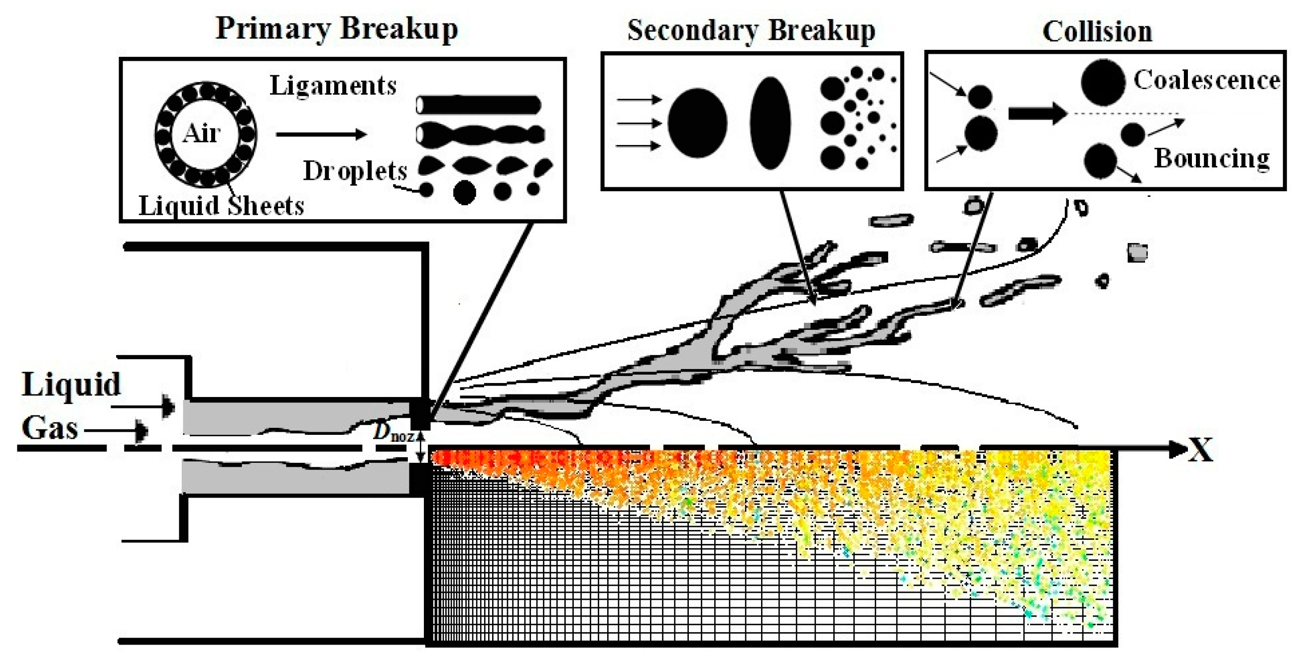
The mathematical model considers two parts. As shown in Figure 1, the first one is the primary breakup sub-model, which predicts gas velocity at the nozzle exit and the droplet mean size. The second sub-model calculates the evolutions of the gas flow and the droplets spray accounting for secondary breakup, collision and coalescence, momentum transfer. The initial droplets characteristics in the second sub-model are provided by the first sub-model calculation. In droplet-gas two-phase flow, the two-way coupling of gas and droplet phase is considered, while the effect of primary breakup jet on the environment gas is neglected.

2.1. Sub-Model of Primary Atomization

The primary atomization is a process that the liquid stream disintegrates into ligaments and drops by interacting with the gas. It is a complex gas-liquid flow. In order to simplify the process, we extracted the main features of the primary atomization from experimental observations.

At present study, effervescent atomizer is chosen since it has so far been found effective for high viscosity liquids [33], in which the gas is introduced into the liquid at low pressure to form a bubbly two-phase mixture upstream of the orifice. As indicated by experimental observation, the flow pattern closed to the nozzle exit is similar to annular. Then, as illustrated in Figure 1, the primary breakup sub-model for effervescent atomizer can be established through three steps.

The first step is estimation of the annular sheets as well as the cylindrical ligaments. The momentum equation of the annular flow combined with the state equation can be written as:

$$RT\ln \left({\mathsf{\rho }}_{g}RT\right)+\frac{1}{2}{\left(\frac{{\dot{m}}_{l}ALR}{{\mathsf{\rho }}_g\mathsf{\pi }{r}_g^2}\right)}^2=\mathrm{const}$$

(1)

where ${\mathsf{\rho }}_g$ is the gas density, $r_g$ is the radius of gas flow, ${\dot{m}}_l$ is the mass flow rate of liquid, and ALR is the air-liquid ratio by mass. The radius of gas flow can be written in terms of orifice radius $r_{\mathrm{orific}}$ and void fraction $\mathsf{\vartheta }$, $r_g=\sqrt{\mathsf{\vartheta }}{r}_{\mathrm{orifice}}$. The interface velocity slip ratio $v_{\mathrm{slip}}$ under different flow rate is expressed as [34]:

$$v_{\mathrm{slip}}=\sqrt{\frac{{\mathsf{\rho }}_l}{{\mathsf{\rho }}_g}\frac{\sqrt{\mathsf{\vartheta }}}{1+C(1-\mathsf{\vartheta })}}$$

(2)

where C is the experimental coefficient of the mass flow rate scaling. The interface velocity slip ratio and void fraction are related by:

$$1+\frac{{\mathsf{\rho }}_{g}sr}{{\mathsf{\rho }}_{l}ALR}=\frac{1}{\mathsf{\vartheta }}$$

(3)

By solving Equations (1)–(3), ${\mathsf{\rho }}_g$, $\mathsf{\vartheta }$ and $v_{\mathrm{slip}}$ can be calculated for different operating conditions. The thickness of annular liquid sheet is then calculated from ${\mathsf{\delta }}_{lig}=4(r_{\mathrm{o}}-r_{\mathrm{g}})/\sqrt{\mathsf{\pi }}$, which is also the diameter of the typical cylindrical ligament. Besides, the gas velocity inside the nozzle orifice can be expressed as $V_{g1}={\dot{m}}_g/(A_{noz}\times \mathsf{\vartheta }\times {\mathsf{\rho }}_g)$, where $A_{noz}$ is the area of the nozzle orifice and ${\dot{m}}_g$ is the gas flow rate. According to the energy conservation equation, the gas velocity at the nozzle exit can be derived from $V_{g2}=\sqrt{{V_{g1}}^2+2RT\log (P_{in}/P_{out})}$, where $R$ is the gas constant, $T$ is the temperature, $P_{in}$ is the pressure inside the nozzle, and $P_{out}$ is the pressure outside the nozzle.

Secondly, the formed ligaments are approximated by cylindrical jets. The ligaments will breakup into fragments at the wavelength of the most rapidly growing wave. The dispersion relations based on instability analysis are used to determine the critical wave number. Here, Joseph’s dispersion relationship [17] is used to describe the linear instability of viscoelastic liquid.

Joseph’s dispersion relationship is derived by considering the acceleration of a drop exposed to a high speed air stream. The equations of ligament motion coupled with boundary conditions are solved to deduce the expression of the disturbed interface:

$$-\left[1+\frac{1}{{\mathsf{\alpha }}^2}(-\dot{a}k+\frac{\mathsf{\sigma }{k}^3}{{\mathsf{\rho }}_l})\right]-4\frac{k^2}{\mathsf{\alpha }}\frac{{\mathsf{\mu }}_{ve}}{{\mathsf{\rho }}_l}+4\frac{k^3}{{\mathsf{\alpha }}^2}{(\frac{{\mathsf{\mu }}_{ve}}{{\mathsf{\rho }}_l})}^2(\sqrt{k^2+{\mathsf{\alpha }\mathsf{\rho }}_l/{\mathsf{\mu }}_{ve}}-k)=0\left({\mathsf{\rho }}_l>>{\mathsf{\rho }}_g\right)$$

(4)

Equation (4) is an approximate analysis of Rayleigh-Taylor instability based on viscoelastic potential flow which gives the critical wavelength and growth rate to within less than 10% of the exact theory. In Equation (4), k is the magnitude of the wave number, $\mathsf{\alpha }$ is the amplification rate, and $\mathsf{\sigma }$ is the liquid surface tension. ${\mathsf{\mu }}_{ve}$ is the effective shear viscosity of the liquid, ${\mathsf{\mu }}_{ve}={\mathsf{\mu }}_0(1+{\mathsf{\alpha }\mathsf{\lambda }}_2)/(1+{\mathsf{\alpha }\mathsf{\lambda }}_1)$ (Section 2.2.2), for viscoelastic liquid, ${\mathsf{\mu }}_{ve}$ is large and ${\mathsf{\alpha }\mathsf{\rho }}_l/(k^2{\mathsf{\mu }}_{ve})<<1$, then $(\sqrt{k^2+{\mathsf{\alpha }\mathsf{\rho }}_l/{\mathsf{\mu }}_{ve}}-k)$ can be assumed to be ${\mathsf{\alpha }\mathsf{\rho }}_l/2k{\mathsf{\mu }}_{ve}$. $\dot{a}$ is the acceleration of the liquid ligament:

$$\dot{a}=\frac{F_{c_d}}{m_{lig}}=\frac{c_d{\mathsf{\rho }}_g{(u_g-u_l)}^2}{{\mathsf{\rho }}_l{\mathsf{\delta }}_{lig}}$$

(5)

where $c_d$ is the drag coefficient. As the ligament Reynolds number $R{e}_{lig}={\mathsf{\rho }}_g{\mathsf{\delta }}_{lig}\left|u_g-u_l\right|/{\mathsf{\mu }}_g$ is between 3 and 1000, here $c_d=24(1+R{e_{lig}}^{2/3}/6)/R{e}_{lig}$. Then, Equation (4) reduces to be a three-degree polynomial of $\mathsf{\alpha }$ as follows and can be solved analytically:

$${\mathsf{\lambda }}_1{\mathsf{\rho }}_l{\mathsf{\alpha }}^3+({\mathsf{\rho }}_l+2{\mathsf{\mu }}_0{\mathsf{\lambda }}_2{k}^2){\mathsf{\alpha }}^2+(2{\mathsf{\mu }}_0{k}^2-\dot{a}k{\mathsf{\rho }}_l{\mathsf{\lambda }}_1+\mathsf{\sigma }{k}^3{\mathsf{\lambda }}_1)\mathsf{\alpha }-\dot{a}k{\mathsf{\rho }}_l+\mathsf{\sigma }{k}^3=0$$

(6)

Based on the above dispersion relation, the critical breakup wave number that corresponds to the maximum growth rate can be used to calculate the wavelength of a typical ligament fragment. Finally, assuming that each fragment is stabilized to one spherical droplet under the influence of surface tension, the Sauter mean drop diameter SMD (defined as the ratio of volume–surface mean diameter ${\displaystyle \sum _i{n}_p}{d}_p^3/{\displaystyle \sum _i{n}_p}{d}_p^2$) can then be calculated from the conservation of mass:

$$SMD={\left[3\mathsf{\pi }\frac{{{\mathsf{\delta }}_{lig}}^2}{k}\right]}^{1/3}$$

(7)

2.2. Sub-Model of Droplet-Gas Two-Phase Flow

The second sub-model is based on hybrid Euler-Lagrangian coordinate system to describe the evolution of spray. The flow field is axisymmetric, and the parcels are tracked in three-dimensional coordinate.

2.2.1. Gas Phase

For the turbulent gas spray, the conservation equations of mass, momentum and energy are written as follows:

$$\{\begin{array}{l}\frac{\partial {\mathsf{\rho }}_g}{\partial t}+\nabla ·\left({\mathsf{\rho }}_g{\mathbf{u}}_{\mathrm{g}}\right)=0\\ \frac{\partial \left({\mathsf{\rho }}_g{\mathbf{u}}_{\mathrm{g}}\right)}{\partial t}+\nabla ·\left({\mathsf{\rho }}_g{\mathbf{u}}_{\mathrm{g}}{\mathbf{u}}_{\mathrm{g}}\right)=-\nabla \left(p+\frac{2}{3}{\mathsf{\rho }}_g\kappa \right)+\nabla ·[{\mathsf{\sigma }}_s]+\mathbf{F}\\ \frac{\partial \left({\mathsf{\rho }}_{g}e\right)}{\partial t}+\nabla ·\left({\mathsf{\rho }}_{g}e{\mathbf{u}}_{\mathrm{g}}\right)=-p\nabla ·{\mathbf{u}}_{\mathrm{g}}-\nabla ·\mathbf{q}+{\mathsf{\rho }}_g\mathsf{\epsilon }+Q\end{array}$$

(8)

where ${\mathbf{u}}_{\mathrm{g}}$ is the gas velocity vector, F is the momentum transfer between the gas and the discrete liquid phase, K is the turbulent kinetic energy per unit mass, ${\mathsf{\sigma }}_s$ is the viscous stress tensor, q is the heat flux vector, $\mathsf{\epsilon }$ is the viscous dissipation rate, and Q is the heat transfer between the gas and the liquid phase. Turbulence effects were modeled by the standard $k-\mathsf{\epsilon }$ model. $F$ and $Q$ are defined as: $\mathbf{F}=-{({\mathsf{\alpha }}_g{V}_{cell})}^{-1}{\displaystyle \sum _P{N}_P{\mathbf{F}}_{\mathrm{p}}}$, $Q={({\mathsf{\alpha }}_g{V}_{cell})}^{-1}{\displaystyle \sum _p{N}_p}\left[Q_p+{\mathbf{F}}_{\mathrm{p}}\left({\mathbf{u}}_{\mathrm{g}}-{\mathbf{u}}_{\mathrm{l}}\right)\right]$, where ${\mathsf{\alpha }}_g$ is the fraction of gas in the computational cell, V_cell is the cell volume, N_p is the number of droplets in this parcel, and F_p is the force acting on each droplet, Q_p is the heat flux through surface of each droplet, and u_l is the droplet velocity.

For the discrete droplets, the momentum equation can be given as: ${\mathbf{F}}_{\mathrm{p}}=\mathsf{\pi }{r}_l^2{\mathsf{\rho }}_l{C}_D\left|{\mathbf{u}}_{\mathrm{g}}-{\mathbf{u}}_{\mathrm{l}}\right|\left({\mathbf{u}}_{\mathrm{g}}-{\mathbf{u}}_{\mathrm{l}}\right)/2$, where F_p is the force exerted on droplet, $m_l$ is the mass of droplet, $r_l$ is the radius of droplet, g is the gravity force, and C_D is the coefficient of the drag force and can be expressed as: $C_D=24/R{e}_l+6(1+R{e}_l^{-1/2})+0.4$. Here the droplets are assumed to be spherical, and the effect of droplet deformation on drag coefficient is not taken into consideration.

2.2.2. Liquid Phase

Secondary Atomization

In this section, we first analyze the constitutive relations of the Newtonian and viscoelastic liquids, introducing more physical properties to describe the viscoelastic contributions. Then, the TAB model which is based on Taylor’s analogy between an oscillating droplet and a spring-mass system was extend to a non-Newtonian version to describe the deformation and distortion of viscoelastic liquids.

For the Newtonian fluid, the shear stress ${\mathsf{\tau }}_{ij}$ can be expressed as:

$${\mathsf{\tau }}_{ij}=-\mathsf{\mu }{d}_{ij}$$

(9)

where $\mathsf{\mu }$ is the Newtonian viscosity, and $d_{ij}$ is the rate of deformation tensor. In cylindrical coordinates, $d_{ij}$ with $(i,j)$ component can be taken as: $d_{ij}=\partial u_r/\partial z+\partial u_z/\partial r$.

For the viscoelastic fluid, according to Jeffreys’ study [35], the rheological model can be expressed with three constants ($\mathsf{\mu },{\mathsf{\lambda }}_1,{\mathsf{\lambda }}_2$) as follows:

$${\mathsf{\tau }}_{ij}+{\mathsf{\lambda }}_1\frac{\partial {\mathsf{\tau }}_{ij}}{\partial t}=-\mathsf{\mu }(d_{ij}+{\mathsf{\lambda }}_2\frac{\partial d_{ij}}{\partial t})$$

(10)

Using the kinetic theory of transient mechanical response in small amplitude motions, the variables $(u_r,u_z)$ in Equations (9) and (10) can be written as $f(r,z,t)=F(r){\mathrm{e}}^{ikz+\mathsf{\alpha }t}$, where $k$ is the wave number, and $\mathsf{\alpha }$ is the growth rate of a perturbation. As deduced by Middleman [15], Equations (9) and (10), respectively become the following:

$$T_{rz}(r)=-\mathsf{\mu }(ik{U}_r(r)+\frac{\mathrm{d}{U}_z(r)}{\mathrm{d}r})$$

(11)

$$T_{rz}(r)=-\mathsf{\mu }\frac{1+{\mathsf{\alpha }\mathsf{\lambda }}_2}{1+{\mathsf{\alpha }\mathsf{\lambda }}_1}(ik{U}_r(r)+\frac{\mathrm{d}{U}_z(r)}{\mathrm{d}r})$$

(12)

By comparing the above two dynamical equations, it concludes that they are identical, the Newtonian viscosity $\mathsf{\mu }$ can be replaced by ${\mathsf{\mu }}_{ve}=\mathsf{\mu }(1+{\mathsf{\alpha }\mathsf{\lambda }}_2)/(1+{\mathsf{\alpha }\mathsf{\lambda }}_1)$ for the viscoelastic model. Based on the above analysis, the original TAB model proposed by Amsden et al. [36] can be used as a foundation for the viscoelastic version. The derivation of viscoelastic version of TAB model include three aspects as below.

First is the modification of deformation equation. The TAB model is based on the Raleigh–Taylor instability analysis, describing the droplet distortion by a forced, damped, harmonic oscillator in which the forcing term is given by the aerodynamic interaction between the droplet and gas; the damping is due to the liquid viscosity, and the restoring force is supplied by the surface tension. Droplet distortion is denoted by the deformation parameter, $\mathsf{\zeta }=2\mathsf{\tau }/r$, where $\mathsf{\tau }$ denotes the change of radial cross-section from its equilibrium position and $r$ is the initial drop radius. The deformation equation of $\mathsf{\zeta }$ in terms of the normalized distortion parameter is:

$$\ddot{\mathsf{\zeta }}+\frac{5{\mathsf{\mu }}_l}{{\mathsf{\rho }}_l{r}^2}\dot{\mathsf{\zeta }}+\frac{8\mathsf{\sigma }}{{\mathsf{\rho }}_l{r}^3}\mathsf{\zeta }=\frac{2{\mathsf{\rho }}_g{\left|U_{rel}\right|}^2}{3{\mathsf{\rho }}_l{r}^2}$$

(13)

where ${\mathsf{\rho }}_l$ is the density, ${\mathsf{\mu }}_l$ is the viscosity, $\mathsf{\sigma }$ is the surface tension, $U_{rel}$ is the relative drop–gas velocity, and the subscripts g and l denote the gas and liquid, respectively. It is assumed that the external aerodynamic force is normal to the drop and the turbulence fluctuations of the surrounding gas are ignored. In reality, there are various modes when droplets breakup as they are subjected to the stresses of the surrounding turbulence gas. However, it is impossible to describe all secondary breakup modes in a single model, therefore only the fundamental mode of oscillation is considered in TAB model.

For a viscoelastic version of TAB model, the constant Newtonian shear viscosity ${\mathsf{\mu }}_l$ was replaced by a viscoelastic viscosity ${\mathsf{\mu }}_{ve}$. In the expression of ${\mathsf{\mu }}_{ve}$, the growth rate of a perturbation $\mathsf{\alpha }$ can be taken by the rate of strain $\dot{\mathsf{\gamma }}$:

$${\mathsf{\mu }}_{ve}={\mathsf{\mu }}_0\frac{1+{\dot{\mathsf{\gamma }}\mathsf{\lambda }}_2}{1+{\dot{\mathsf{\gamma }}\mathsf{\lambda }}_1}$$

(14)

where ${\mathsf{\lambda }}_1$ is the fluid relaxation time, ${\mathsf{\lambda }}_2$ is the retardation time, and ${\mathsf{\mu }}_0$ is the zero shear viscosity. The rate of strain $\dot{\mathsf{\gamma }}$ is approximated as $\dot{\mathsf{\gamma }}=U_{rel}/2r_0$. As indicated in Equation (14), on the one hand, ${\mathsf{\mu }}_{ve}$ will approach zero shear viscosity ${\mathsf{\mu }}_0$ when the rate of strain $\dot{\mathsf{\gamma }}$ is close to 0. On the other hand, ${\mathsf{\mu }}_{ve}$ will approach ${\mathsf{\mu }}_0{\mathsf{\lambda }}_2{/\mathsf{\lambda }}_1$ when $\dot{\mathsf{\gamma }}$ becomes larger. Therefore, when ${\mathsf{\lambda }}_2<{\mathsf{\lambda }}_1$ and the rate of strain is increasing, ${\mathsf{\mu }}_{ve}<{\mathsf{\mu }}_0$, which means that the liquid is shear thinning. For dilute polymer solutions, the relationship of retardation time and relaxation time is ${\mathsf{\lambda }}_2={\mathsf{\lambda }}_1{\mathsf{\eta }}_{solvent}/{\mathsf{\eta }}_{solution}$ [37], where ${\mathsf{\eta }}_{solvent}$ and ${\mathsf{\eta }}_{solution}$ are the viscosity of solvent and solution, respectively.

Second, the breakup criterion is changed. In TAB model, drop breakup occurs when the normalized drop distortion $\mathsf{\zeta }\left(t\right)$ exceeds the critical value of 1. For Newtonian droplet, the stability limit has been determined experimentally to be $W{e}_g={\mathsf{\rho }}_g{U}_{rel}^{2}r/\mathsf{\sigma }=6$. For high viscous liquid, the effect of viscosity on the stability should be related to the breakup criterion. As proposed by Brodkey [38], the critical Weber number can be modified by introducing the Ohnesorge number:

$$W{e}_{g.crit}=6(1+1.077O{h}^{1.6}),Oh={\mathsf{\mu }}_l/\sqrt{2{\mathsf{\rho }}_l\mathsf{\sigma }r}$$

(15)

when $Oh\le 0.1$, the value of this expression approximates to 6, which means the case of low viscosity for Newtonian liquid is recovered. When $Oh$ is higher, the stability limit is increased and scales as ${\mathsf{\mu }}_l^{1.6}$ in the asymptotic limit. Based on the Brodkey’s empirical relation, an effective Weber number is introduced to instead of the regular one [38]:

$$W{e}_g^{eff}=\frac{W{e}_g}{1+1.077O{h}^{1.6}}$$

(16)

for the viscoelastic liquid, ${\mathsf{\mu }}_{ve}$ is used instead of ${\mathsf{\mu }}_l$ in $Oh$ number.

Third, the creation of the product droplets is also revised. The population dynamics is used to define the rate of droplet creation. For each breakup event, with the mass conservation principle, it is assumed that the number of product droplets is proportional to the number of critical parent drops, where the proportionality constant depends on the drop breakup regime:

$$\frac{\mathrm{d}}{\mathrm{d}t}\overline{m}(t)=-3K_{bu}\overline{m}(t)$$

(17)

where $\overline{m}(t)$ denotes the mean mass of the product drop distribution, and the breakup frequency $K_{bu}$ depends on the drop breakup regimes. Breakup frequency $K_{bu}=0.05\mathsf{\omega }$ as suggested by Amsden et al. [36] is used. The drop oscillation frequency $\mathsf{\omega }$ is given by ${\mathsf{\omega }}^2=8\mathsf{\sigma }/({\mathsf{\rho }}_l{r}^3)-25{\mathsf{\mu }}_l^2/(4{\mathsf{\rho }}_l^2{r}^4)$, where ${\mathsf{\mu }}_l$ is also replaced by ${\mathsf{\mu }}_{ve}$ for viscoelastic version.

Droplets Collision

Droplet collision is calculated by a statistical method, rather than a deterministic method since the real collisions process is highly stochastic. All the droplets in one computational parcel behave in the same manner, they either do or do not collide, which is depended on the probability of the collision whether larger than a random number. For collision result, an impact parameter, $\mathsf{\psi }=\mathsf{\chi }/(r_1+r_2)$ is involved to judge the outcomes, where $\mathsf{\chi }$ is the distance between the center of one drop and the relative velocity vector $U_{rel}$, $r_1$ and $r_2$ are the radii of small and large droplets, respectively. The criteria, ${\mathsf{\chi }}_{cr}$ determines the transition boundary: drops coalescence when $\mathsf{\chi }\le {\mathsf{\chi }}_{cr}$, and bounce when $\mathsf{\chi }>{\mathsf{\chi }}_{cr}$. ${\mathsf{\chi }}_{cr}$ can be expressed as:

$${{\mathsf{\chi }}_{cr}}^2={(r_1+r_2)}^2\min \left[1.0,2.4f(\mathsf{\gamma })/W{e}_l\right]$$

(18)

where the collision Weber number for Newtonian liquid defined as: $W{e}_l={\mathsf{\rho }}_l\left|{\mathit{U}}_{rel}\right|r_1/{\mathsf{\sigma }}_l$. For viscoelastic liquid, $W{e}_l^{eff}=W{e}_l/(1+1.077O{h}^{1.6})$ is used instead of $W{e}_l$. $f(\mathsf{\gamma })$ is a function of the radius ratio $\mathsf{\gamma }$: $f(\mathsf{\gamma })={\mathsf{\gamma }}^3-2.4{\mathsf{\gamma }}^2+2.7\mathsf{\gamma }$ $(\mathsf{\gamma }=r_2/r_1\ge 1)$.

According to the conservation of momentum, the drop velocity after a bouncing collision is [36]: $u_{1new}=\{u_1{m}_1+u_2{m}_2+m_2(u_1-u_2)[(\mathsf{\chi }-{\mathsf{\chi }}_{cr})/(r_1+r_2-{\mathsf{\chi }}_{cr})]\}/(m_1+m_2)$. The droplet velocity after coalescence is calculated as $u_{new}=(u_1{m}_1+u_2{m}_2)/(m_1+m_2)$. $m_1$ and $m_2$ are the mass of the small and large droplets, respectively; and $u_1$ and $u_2$ are the velocity of the small and large droplets, respectively. The new radius after droplet coalescence is $r_{new}={(r_1^3+r_2^3)}^{1/3}$.

3. Numerical Setup

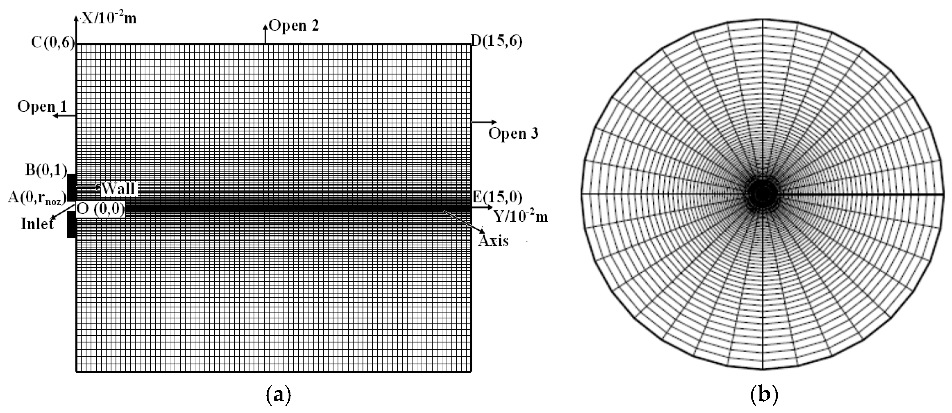
Figure 2 shows the computational mesh and boundary conditions of numerical model. The radius and axial lengths of the computational regime are 6 cm and 15 cm respectively, and 2$\mathsf{\pi }$ in the circular direction. The computational domain is in a cylindrical coordinate system with size of 56 (radial) × 65 (axial) × 32 (azimuthal). Finer meshes are used for the core region of the spray. The grid dependency has been validated in our previous studies [39,40] and the computational results are convergence under present mesh size.

As presented in

Table 1. Five types of boundary conditions involved in the model.

Type		Location	Conditions
Open	1	Line BC	$\mathit{v}\left(x,0,\mathsf{\theta }\right)>0$: $P$, $T$, $u$ are assigned the same as that in ambient
			$\mathit{v}\left(x,0,\mathsf{\theta }\right)\le 0$: $\partial u/\partial y=0$, $\partial \mathsf{\varphi }/\partial y=0$ ($\mathsf{\varphi }=P,T$)
	2	Line CD	$\mathit{u}\left(6,y,\mathsf{\theta }\right)<0$: $P$, $T$, $\mathit{v}$ are assigned the same as that in ambient
			$\mathit{u}\left(6,y,\mathsf{\theta }\right)\ge 0$: $\partial \mathsf{\varphi }/\partial x=0$, $\partial v/\partial y=0$
	3	Line DE	$\mathit{v}\left(x,15,\mathsf{\theta }\right)<0$: $P$, $T$, $u$ are assigned the same as that in ambient
			$\mathit{v}\left(x,15,\mathsf{\theta }\right)\ge 0$: $\partial u/\partial y=0$, $\partial \mathsf{\varphi }/\partial y=0$
Wall		Line AB	$u,v,w=0$; $T=300\mathrm{K}$; turbulent wall function
Inlet		Line OA	Data from primary breakup sub-model
Axis		x = 0	${\mathsf{\xi }|}_{x=0}=({\displaystyle \sum _{i=1}^N{\mathsf{\xi }}_i})/N$ ($\mathsf{\xi }=u,v,T$, ${\mathsf{\xi }}_i$: $\mathsf{\xi }$ at $\Delta x$ from the centerline); $w=0$
Periodic		θ = 2π	Circular direction: periodic boundary conditions

, there are five types of boundary conditions involved for the gas field. The parcels are introduced in the system at the nozzle exit, which has the original size calculated from primary breakup sub-model with Rosin-Rammler distribution: $F_{R-R}(D)=1-\exp \{-{(D/SM{D}_0)}^{q_{co}}\}$, where $q$_co indicates the value of the width of the distribution. The Rosin-Rammler distribution is a prevalent size distribution used in the atomization field [41], and the experimental data also supported the Rosin-Rammler function for non-Newtonian fluid atomization spray [31]. The number of parcels should be large enough to reduce statistical fluctuation. Usually, a total number of 10,000 computational parcels are injected into the flow for each case.

4. Results and Discussion

4.1. Validation of Primary Atomization

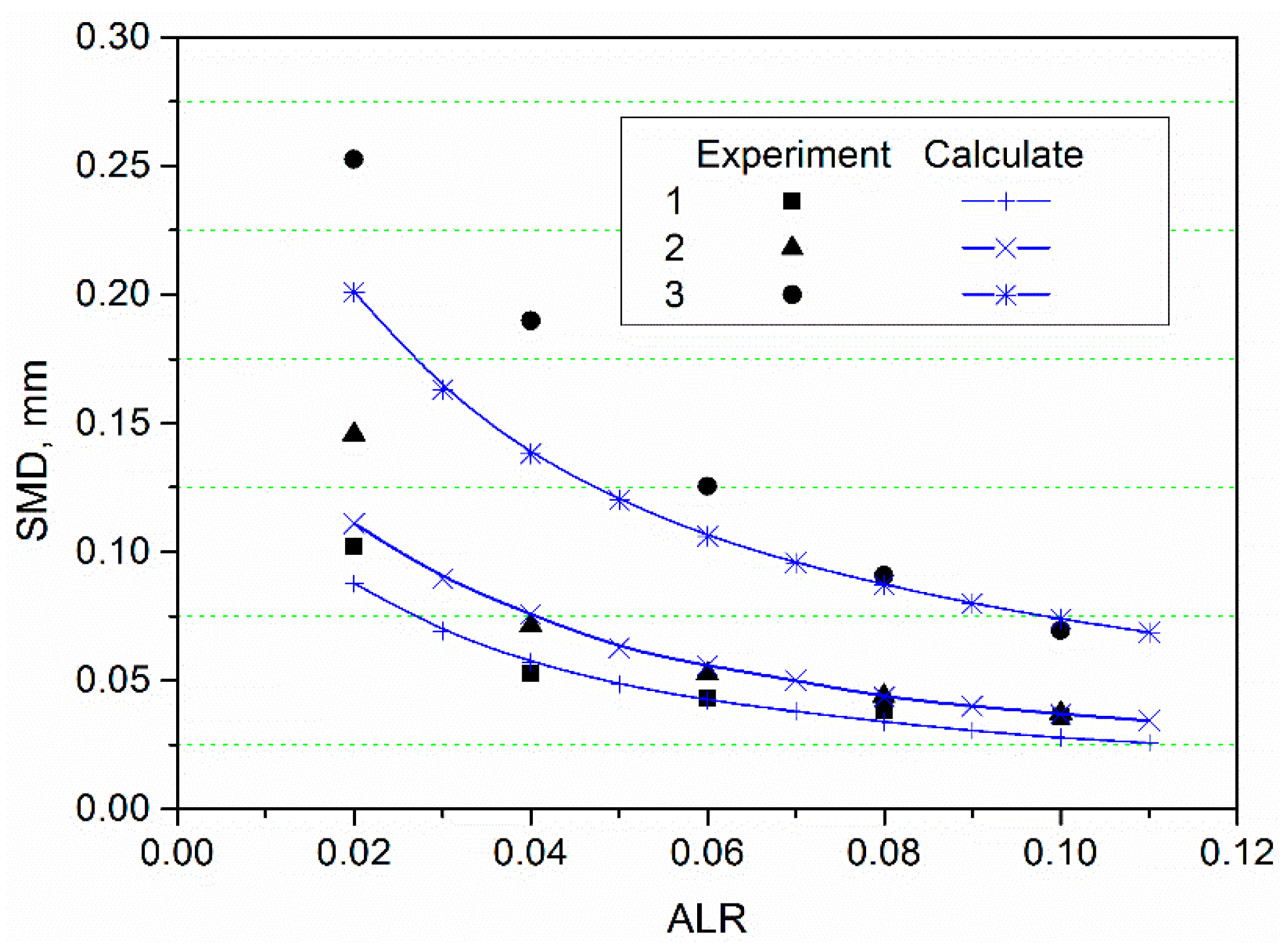
Figure 3 shows a comparison of experimental data [42] and model predictions for polymer solution atomization at $P_{inj}=0.35\mathrm{MPa}$, $D_{noz}=1\mathrm{mm}$ and ALR ranging from 0.02 to 0.11. The physical and rheological properties are listed in

Table 2. Physical properties of the fluids in Figure 3 [42].

Code	Polymer Concentration	Zero Shear Viscosity ${\mathsf{\eta }}_0$	Relaxation Time ${\mathsf{\lambda }}_1$	Surface Tension $\mathsf{\sigma }$
		mPa·s	s	10−3 J/m2
1	0.001%	11	2.8 × 10−7	65.1
2	0.01%	11.1	1.4 × 10−5	62.6
3	0.15%	15.4	2.06 × 10−4	62.6

. The polymer solution were formulated by adding poly(ethylene oxide) to solvent having a common composition of 60% glycerine–40% water solution by mass. Polyethylene oxide (PEO) molecular weights of 100,000 were used at mass concentrations of 0.001%, 0.01% and 0.15% [42]. The dispersion relations proposed by Joseph are solved analytically. Results show that, with an increase in air–liquid mass flow ratio (ALR), droplet SMD will decline significantly, especially at lower ALR. The agreement between the predictions and measurements is qualitative achieved within 5%–20%. Joseph’s model is effective to capture the influence of rheological properties on the breakup process of polymer solution and to quantitatively predict the resulting droplet sizes. However the shortcoming is that the divergence may occur when the liquid ligament is not similar to the flattened drop. Therefore, at lower ALR, the divergence is obviously since the liquid ligaments is slender.

4.2. Evolution of Spray Field

Among the investigations of the far-field region, the particle size evolution along with the axial distance is the primary interest. Figure 4 firstly validates the numerical results of water’s SMD with experimental data [43] and then compares the downstream variation of SMD for water and polymer solution. Both experiment and simulations were conducted based on the same operating conditions. The operating parameters and liquid physical properties are listed in

Table 3. Operating parameters and liquid physical properties of baseline case.

Parameters	Value	Parameters	Value
$D_{noz}$ $\left(\mathrm{mm}\right)$	1	${\mathsf{\eta }}_0$ $({10}^{-3}\mathrm{Pa}·\mathrm{s})$	15
$\mathsf{\sigma }$ $({10}^{-3}{\mathrm{J}/\mathrm{m}}^2)$	65	${\mathsf{\eta }}_{solvent}$ $({10}^{-3}\mathrm{Pa}·\mathrm{s})$	10
$ALR$	0.06	${\mathsf{\lambda }}_1$ $\left(\mathrm{s}\right)$	2.0 × 10-6
${\dot{m}}_l$ $(\mathrm{g}/\mathrm{s})$	10	$P_{inj}$ $({10}^6\mathrm{Pa})$	0.35

.

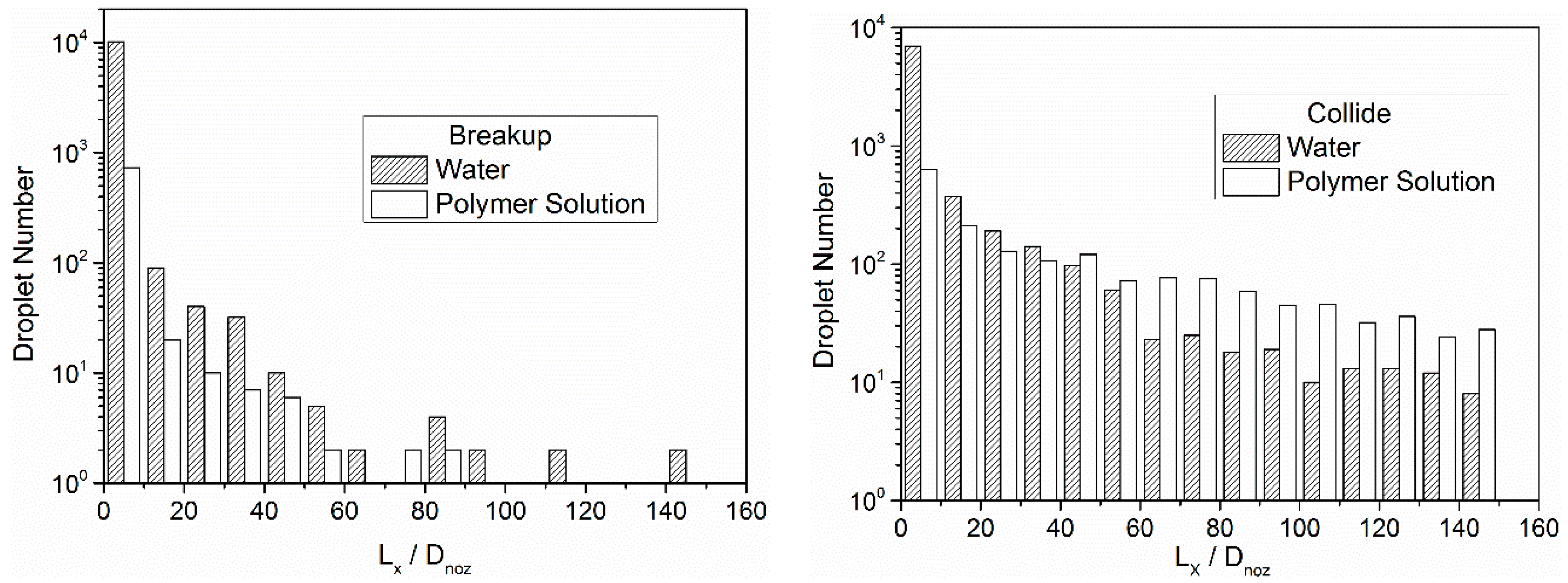
As shown in Figure 4, an agreement between the simulation results and experimental data has been obtained for the case of water, and the divergence of the experiment and simulation is between 2.5% and 25%. In Figure 4, the viscoelastic liquid added the difficulties in the breakup of ligaments and droplets, impairing the atomization effect by increasing the drop size in the whole process, which is consistent with the results of other researchers [12,44]. Further, in both the cases of water and polymer solution, the droplet diameter first decreases and then increases with the axial distance. This phenomenon can be explained by the competition between breakup and coalescence effects. Figure 5 shows the occurrence number of droplets breakup and collision. Close to the nozzle exit, with high kinetic energy and large velocity difference between the droplet and atomization gas, turbulence breakup dominates, causing the drop size to rapidly decrease, while, further downstream, as the kinetic energy decay and small velocity difference, turbulence breakup ends and droplet coalescence plays an important role, causing the drop size to gradually increase.

Besides the common and well-known points, there are two noteworthy differences between these two types of liquids. First, in Figure 4, the gap between the mean size of water and polymer solution is shortened along with the development of the jet. Before the nadir of the curve, the case of polymer solution decays more steeply than that of water. In contrast, after the nadir of the curve, the case of water rises more obviously than that of polymer solution. On the rising part of the curves, the increasing degree of water is about 123%, while the case of polymer solution is less than 57% (this value is calculated from $(SM{D}_{L_x/D_{noz}=140}-SM{D}_{L_x/D_{noz}=4})/SM{D}_{L_x/D_{noz}=4}$). This phenomenon indicates that the mean size of polymer solution increases more gently than that of water at the axial distance $(5–100)L_x/D_{noz}$, which is benefit to control the desirable size in industrial applications. Secondly, in Figure 5, the occurrence numbers for water are higher than polymer solutions for both breakup and collision process in the upstream of the spray. This is because droplets breakup time and frequency depend on the competition between the aerodynamic force and restoring force. An increase in liquid viscosity will delay and weaken the breakup process, resulting in higher droplet size. The decrease of the frequency of droplet secondary breakup would also lead to the number of product droplets decreasing, therefore the collision occurrence number of polymer solutions is obviously less than that of water in the upstream region. However, when the axial distance beyond $40L_x/D_{noz}$, the collision occurrence number for polymer solution exceeds that of water. Since the droplets collision process were influenced by the droplet size and concentration rate. Concentrated drop distribution causes the collision happening frequently. The outcome of collision was also affected by the liquid viscosity. For the polymer solution droplets, impact parameter increased due to higher viscosity, leading to an increase in possibility of droplet coalescence after collision. However, the change of collision occurrence number did not influence the trend of SMD in Figure 4 significantly, due to the occurrence number is too small compared to the total particle number.

The most important factors influencing the droplet breakup can be grouped into two dimensionless numbers, the Weber number ($We$) and the Ohnesorge number ($Oh$). The average Weber number is defined as $We={\mathsf{\rho }}_g{\left|{\overline{\mathit{U}}}_{rel}\right|}^{2}SMD/{\mathsf{\sigma }}_l$. Here the modified weber number (Equation (16)) is used for the polymer solution. The average Ohnesorge number is expressed as $Oh={\mathsf{\mu }}_l/\sqrt{{\mathsf{\rho }}_l{\mathsf{\sigma }}_{l}SMD}$. For viscoelastic liquid, the constant viscosity ${\mathsf{\mu }}_l$ was replaced by a viscoelastic viscosity ${\mathsf{\mu }}_{ve}$.

The evolutions of Weber and Ohnesorge number along with the axial direction are illustrated in Figure 6. Weber number indicates the ratio of the inertial force to the surface tension force, in which the trend is basically determined by the gas-liquid relative velocity. At the nozzle exit, $We$ is higher due to the large difference between the velocity of droplet and gas, causing the secondary breakup of droplets. In this period, $We$ of polymer solution is larger than that of water due to the larger SMD at the beginning. Then at downstream of the spray, $We$ dramatically declines as the kinetic energy dissipated and $We$ of polymer solution is less than that of water since $We$ for viscoelastic liquid is modified by the effective viscosity. The effective Weber number decreased as liquid viscosity increasing. The Ohnesorge number is the ratio of an internal viscosity force to an interfacial surface tension force, which significantly increases with the increase of liquid viscosity. For both water and polymer solution, the $Oh$ curves have a peak at about 4 mm from the nozzle exit, which is corresponding to the nadir of the curve of droplet size (as shown in Figure 4). In short, the case of polymer solution has a greater magnitude of change for both $We$ and $Oh$ due to introducing the changes in viscosity.

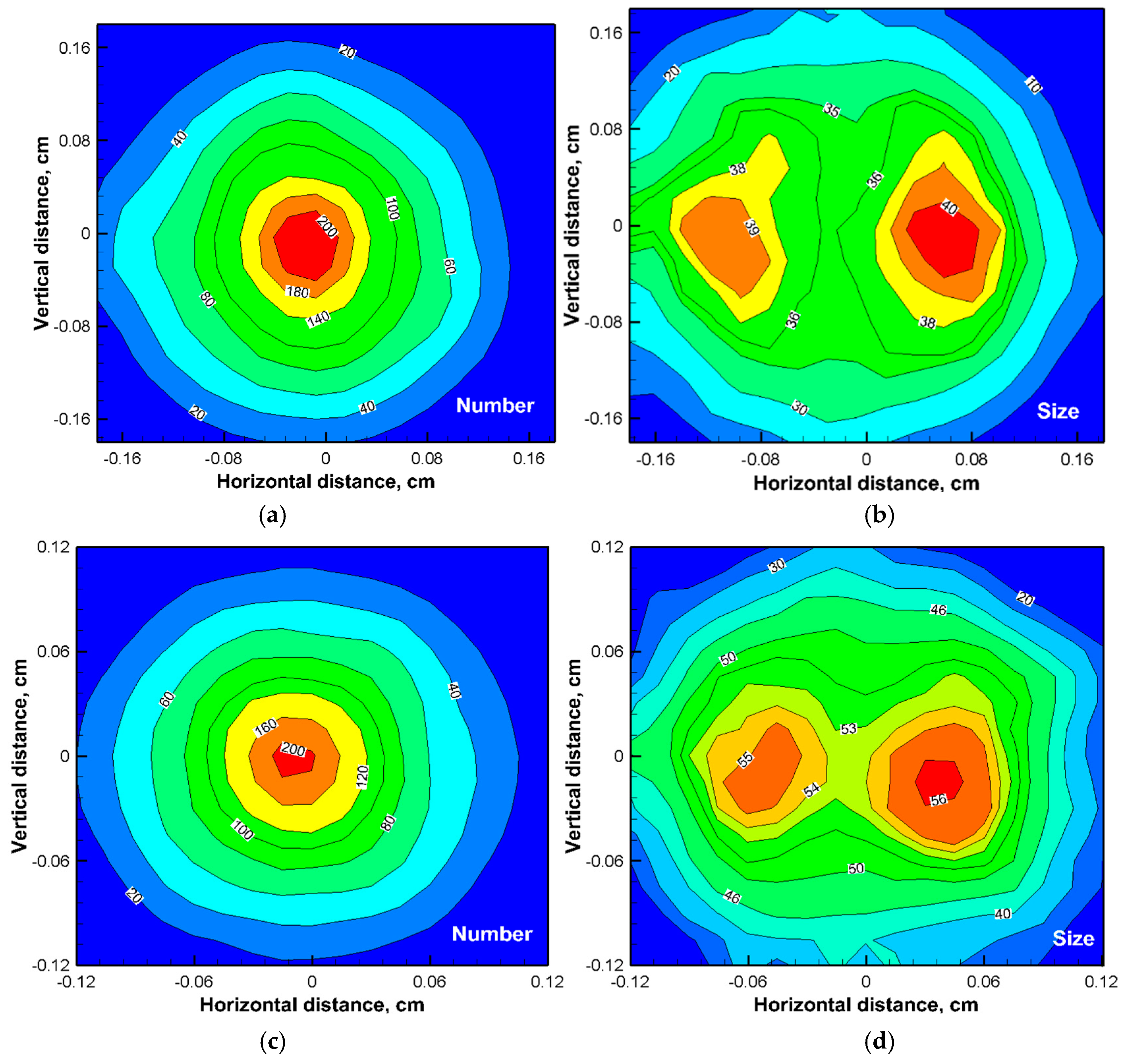
In addition to drop size and critical numbers, liquid viscosity can also affect the spray pattern. Figure 7 shows the spatial distributions of droplet size and number for water and polymer solution, respectively. The cross-sectional plane is located at the axial distance of 50 mm. It can be seen from Figure 7 that the spatial distribution of droplets becomes wider for water. The distribution range of water case is about 40% larger than the polymer solution. It can be explained as the ligaments and fragments are more likely to adhere due to viscoelastic properties. Furthermore, finer droplets are easier for the gas to accelerate and carry them outward of the centerline, resulting in the spray angle will expand. In turn, the distribution will also affect the droplet size. Concentrated drop distribution causes the collision happening frequently and the droplet size increasing, which is in accordance with that indicated in Figure 5.

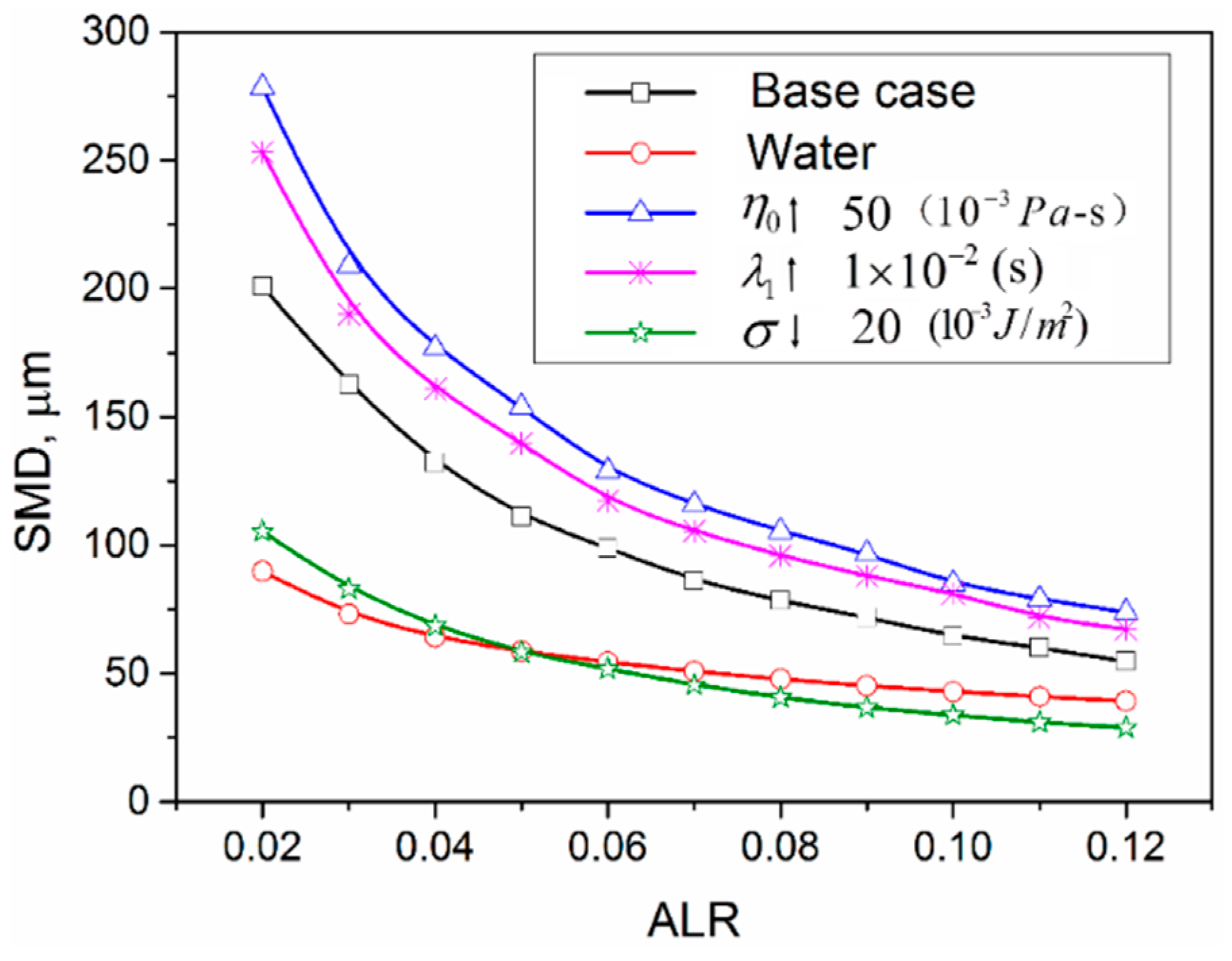
4.3. Effects of Viscoelastic Parameters

Figure 8 shows the analysis of the effects of rheological properties on primary atomization. Figure 9 explores the evolutions of droplet size along with axial direction for various liquid properties. For polymer solutions, the rheology properties can be adjusted through the addition of polymer molecules. The liquid physical properties of base case are as the same as that of code 2 in Table 2. All cases in Figure 8 and Figure 9 share the same operating conditions except the specified parameters in the legend of the figure. In order to compare the behavior of Newtonian and viscoelastic liquid, the calculated results of water spray have been added into Figure 8 and Figure 9.

Obviously, from Figure 8 and Figure 9, the increases in relaxation time and zero-shear viscosity cause the atomization quality deteriorates since the growth rate of the disturbance wave reduces and the liquid becomes stringier to resist the disruptive force, while small surface tension brings the droplet size to decrease significantly. The case with surface tension of $20\times {10}^{-3}{\mathrm{J}/\mathrm{m}}^2$ is almost identical to the case of water. In both instability analysis and TAB model, the surface tension can resist the occurrence and development of instability and smooth the disturbance. That is, a decrease in surface tension brings the ligaments and droplet less stability. This finding shows the importance of selecting solvents with lower surface tension for the polymer solution when finer atomization effects are desirable. Moreover, the effects of relaxation time become weaken at the downstream of the spray field. The case with shorter relaxation time approaches to the base case since the influence of relaxation time depends on the gas-liquid relative velocity. When the relative velocity declined rapidly, the effective viscosity of viscoelastic liquid is mainly up to zero shear viscosity.

5. Conclusions

A comprehensive mathematical model has been proposed to simulate the outflow of the effervescent atomization for viscoelastic liquid, accounting for primary atomization droplet tracking, secondary breakup and droplet collision. The computational models have included two parts. The first one is the primary breakup sub-model. With the simplification and assumptions of the atomization of liquid stream, the primary breakup sub-model has been established based on the viscoelastic linear dispersion relation. The second sub-model can calculate the evolutions of the droplets spray, in which the gas-liquid two-phase flow has been simulated by the Euler-Lagrangian approach. Both the droplet secondary atomization model and collision model have been extended to the viscoelastic version by introducing rheological parameters. The main findings of the present study can be summarized in four points:

(1)

Based on the comparison with experimental data and the predicted results of other dispersion relation, the primary model using Joseph’s relation effectively captured the influence of rheological properties on the breakup process of polymer solution and to quantitatively predict the resulting droplet sizes.

(2)

The evolutionary trend of droplet mean diameter, Weber number and Ohnesorge number of viscoelastic liquids along with axial direction were qualitatively similar to that of Newtonian liquids. The SMD for the case of polymer solutions were obviously larger than that of water throughout the spray field. While, the gap of SMD between water and polymer solution became shorten along with the development of the jet. This phenomenon indicated that the mean size of polymer solution increased more gently than that of water at the axial distance $(5–100)L_x/D_{noz}$, which benefited the stable control of the desirable size in the applications.

(3)

The changes of Weber and Ohnesorge number for polymer solution were more dramatic than that of water, since the viscosity of the viscoelastic liquid was influenced by the relative velocity of gas and droplets. Besides, the distribution range of water was about 40% larger than that of polymer solution in present study, which indicated the spray angle became narrow for the viscoelastic liquids.

(4)

In primary atomization, the surface tension was the dominating physical property for viscoelastic liquid rather than relaxation time and zero shear viscosity. When the finer atomization effects were desirable, it was important to select solvents with lower surface tension for the polymer solutions, while, concerning the evolution of atomization spray, larger relaxation time and zero shear viscosity increased droplet SMD significantly. The zero shear viscosity was effective throughout the jet region, while the effect of relaxation time became weaken at the downstream of the spray field.

References

- Mallory, J.A. Jet Impingement and Primary Atomization of Non-Newtonian Liquids. Ph.D. Thesis, Purdue University, West Lafayette, IN, USA, 2012. [Google Scholar]
- Yoo, H.; Kim, C. Generation of inkjet droplet of non-Newtonian fluid. Rheol. Acta 2013, 52, 313–325. [Google Scholar] [CrossRef]
- Hoath, S.D.; Vadillo, D.C.; Harlen, O.G.; Mcllroy, C.; Morrison, N.F.; Hsiao, W.; Tuladhar, T.R.; Jung, S.; Martin, G.D.; Hutchings, I.M. Inkjet printing of weakly elastic polymer solution. J. Non-Newton. Fluid Mech. 2014, 205, 1–10. [Google Scholar] [CrossRef]
- Petersen, F.J.; Wørts, O.; Schæfer, T.; Sojka, P.E. Effervescent atomization of aqueous polymer solutions and dispersions. Pharm. Dev. Technol. 2001, 6, 201–210. [Google Scholar] [CrossRef] [PubMed]
- Pawlowski, L. Suspension and solution thermal spray coatings. Surf. Coat. Technol. 2009, 203, 2807–2829. [Google Scholar] [CrossRef]
- Bartolo, D.; Boudaoud, A.; Narcy, G.; Bonn, D. Dynamics of non-newtonian droplets. Phys. Rev. Lett. 2007, 99, 174502. [Google Scholar] [CrossRef] [PubMed]
- Schowalter, W.R. Mechanics of Non-Newtonian Fluids; Pergamon Press: Oxford, UK, 1978. [Google Scholar]
- Oldroyd, O.G. Non-Newtonian effects in steady motion of some idealized elastic viscous fluids. Proc. R. Soc. 1958, 279, A245. [Google Scholar]
- Li, L.K.B.; Dressler, D.M.; Green, S.I.; Davy, M.H.; Eadie, D.T. Experiments on air-blast atomization of viscoelastic liquids, Part 1: Quiescent conditions. At. Sprays 2009, 19, 157–190. [Google Scholar] [CrossRef]
- Dumouchel, C. On the experimental investigation on primary atomization of liquid streams. Exp. Fluids 2008, 45, 371–422. [Google Scholar] [CrossRef]
- Aliseda, A.; Hopfinger, E.J.; Lasheras, J.C.; Kremer, D.M.; Berchielli, A.; Connolly, E.K. Atomization of viscous and non-newtonian liquids by a coaxial, high-speed gas jet: Experiments and droplet size modeling. Int. J. Multiph. Flow 2008, 34, 161–175. [Google Scholar] [CrossRef]
- Harrison, G.M.; Mun, R.P.; Cooper, G.; Boger, D.V. A note on the effect of polymer rigidity and concentration on spray atomization. J. Non-Newton. Fluid Mech. 1999, 85, 93–104. [Google Scholar] [CrossRef]
- Chao, K.K.; Child, C.A.; Grens, E.A., II; Williams, M.C. Anti-misting action of polymeric additives in jet fuels. AIChE J. 1984, 30, 111–120. [Google Scholar] [CrossRef]
- Sirignano, W.A.; Mehring, C. Review of theory of distortion and disintegration of liquid streams. Prog. Energy Combust. Sci. 2000, 26, 609–655. [Google Scholar] [CrossRef]
- Middleman, S. Stability of a viscoelastic jet. Chem. Eng. Sci. 1965, 20, 1037–1040. [Google Scholar] [CrossRef]
- Goren, S.L.; Gorttlieb, M. Surface-tension driven breakup of viscoelastic liquid threads. J. Fluid Mech. 1982, 120, 245–266. [Google Scholar] [CrossRef]
- Joseph, G.E.; Funda, B.T. Rayleigh-Taylor instability of viscoelastic drops at high Weber number. J. Fluid Mech. 2002, 453, 109–132. [Google Scholar] [CrossRef]
- Yang, L.J.; Tong, M.X.; Fu, Q.F. Linear stability analysis of a three-dimensional viscoelastic liquid jet surrounded by a swirling air stream. J. Non-Newton. Fluid Mech. 2013, 191, 1–13. [Google Scholar] [CrossRef]
- Fuster, D.; Bagué, A.; Boeck, T.; Le Moyner, L.; Leboissetier, A.; Popinet, S.; Scardovelli, R.; Zaleski, S. Simulation of primary atomization with an octree adaptive mesh refinement and VOF method. Int. J. Multiph. Flow 2009, 35, 550–565. [Google Scholar] [CrossRef]
- Villermaux, E. Fragmentation. Annu. Rev. Fluid Mech. 2007, 39, 419–446. [Google Scholar] [CrossRef]
- Gorokhovski, M.; Herrmann, M. Modeling primary atomization. Annu. Rev. Fluid Mech. 2008, 40, 343–366. [Google Scholar] [CrossRef]
- Zhu, C.; Ertl, M.; Weigand, B. Numerical investigation on the primary breakup of an inelastic non-Newtonian liquid jet with inflow turbulence. Phys. Fluids 2013, 25, 083102. [Google Scholar] [CrossRef]
- Stelter, M.; Brenn, G.; Durst, F. The influence of viscoelastic fluid properties on spray formation from flat-fan and pressure-swirl atomizers. At. Sprays 2002, 12, 299–327. [Google Scholar] [CrossRef]
- Dexter, R.W. Measurement of extensional viscosity of polymer solutions and its effects on atomization from a spray nozzle. At. Sprays 1996, 6, 167–191. [Google Scholar] [CrossRef]
- Hartranft, T.J.; Settles, G.S. Sheet atomization of non-Newtonian liquids. At. Sprays 2003, 13, 191–221. [Google Scholar] [CrossRef]
- Mun, R.P.; Young, B.W.; Boger, D.V. Atomization of dilute polymer solutions in agricultural spray nozzles. J. Non-Newton. Fluid Mech. 1999, 83, 163–178. [Google Scholar] [CrossRef]
- Rivera, C.L. Secondary Breakup of Inelastic Non-Newtonian Liquid Drops. Ph.D. Thesis, Purdue University, West Lafayette, IN, USA, 2010. [Google Scholar]
- Dechelette, A.; Campanellab, O.; Corvalanc, C.; Sojka, P.E. An experimental investigation on the breakup of surfactant-laden non-Newtonian jets. Chem. Eng. Sci. 2011, 66, 6367–6374. [Google Scholar] [CrossRef]
- Ma, Y.; Bai, F.; Chang, Q.; Yi, J.; Jiao, K.; Du, Q. An experimental study on the atomization characteristics of impinging jets of power law fluid. J. Non-Newton. Fluid Mech. 2015, 217, 49–57. [Google Scholar] [CrossRef]
- Xue, Z.; Carlos, M.C.; Dravid, V.; Sojka, P.E. Breakup of shear-thinning liquid jets with surfactants. Chem. Eng. Sci. 2008, 63, 1842–1849. [Google Scholar] [CrossRef]
- Mallory, J.; Sojka, P.E. On the primary atomization of non-Newtonian imping jets: Volume II linear stability theory. At. Sprays 2014, 24, 525–554. [Google Scholar] [CrossRef]
- Ashgriz, N. Handbook of Atomization and Sprays: Theory and Applications; Springer: New York, NY, USA, 2011. [Google Scholar]
- Broniarz-Press, L.; Ochowiak, M.; Woziwodzki, S. Atomization of PEO aqueous solutions in effervescent atomizers. Int. J. Heat Fluid Flow 2010, 31, 651–658. [Google Scholar] [CrossRef]
- Lund, M.T.; Jian, C.Q. The influence of atomizing gas molecular weight on low mass flow-rate effervescent atomization performance. J. Fluids Eng. 1998, 120, 750–754. [Google Scholar] [CrossRef]
- Bird, R.B. Useful non-Newtonian models. Annu. Rev. Fluid Mech. 1976, 8, 13–34. [Google Scholar] [CrossRef]
- Amsden, A.A.; O’Rourke, P.J.; Butler, T.D. KIVA-II: A Computer Program for Chemically Reactive Flows with Sprays; Technical Report LA-11560-MS; Los Alamos National Laboratory: Los Alamos, NM, USA, 1980. [Google Scholar]
- Denn, M.M. Issues in viscoelastic fluid mechanics. Annu. Rev. Fluid Mech. 1999, 22, 13–32. [Google Scholar] [CrossRef]
- Brodkey, R.S. The Phenomena of Fluid Motions, Addison-Wesley Series in Chemical Engineering; Addison-Wesley: New York, NY, USA, 1967. [Google Scholar]
- Xiong, H.B.; Lin, J.Z.; Zhu, Z.F. Three-dimensional simulation of effervescent atomization spray. At. Sprays 2009, 19, 1–16. [Google Scholar] [CrossRef]
- Lin, J.Z.; Qian, L.J.; Xiong, H.B.; Chan, T.L. Effects of operating conditions on droplet deposition onto surface of atomization impinging spray. Surf. Coat. Technol. 2009, 203, 1733–1740. [Google Scholar] [CrossRef]
- Lefebvre, A.H. Atomization and Sprays; Hemisphere Publishing Corporation: Carlbad, CA, USA, 1989. [Google Scholar]
- Geckler, S.C.; Sojka, P.E. Effervescent atomization of viscoelastic liquids: Experiments and modeling. J. Fluids Eng. 2008, 130, 061303. [Google Scholar] [CrossRef]
- Liu, L.S. Experimental and Theoretical Investigation on the Characteristics and Two-Phase Spray Flow Field of Effervescent Atomizers. Ph.D. Thesis, Tianjing University, Tianjin, China, 2001. [Google Scholar]
- Mansour, A.; Chigier, N. Air-Blast atomization of Non-Newtonian liquids. J. Non-Newton. Fluid Mech. 1995, 58, 161–194. [Google Scholar] [CrossRef]
Figure 1.
Schematic of the effervescent atomization spray.
Figure 2.
Geometry and computational mesh: a middle section plane. (a) Middle section plane; and (b) Cross section plane.
Figure 3.
Comparison of experimental data and model predictions for the Sauter mean diameter (SMD) versus air-liquid mass flow ratio (ALR) at , .
Figure 4.
Droplet Sauter mean diameter along with the dimensionless axial distance for water and polymer solution.
Figure 5.
Occurrence number of droplets breakup and collision.
Figure 6.
Evolutions of Weber and Ohnesorge number along with axial direction for water and polymer solution.
Figure 7.
Spatial distribution of the drop number and size at the axial distance of 50 mm. (a) Number distribution of water; (b) Size distribution of water ; (c) Number distribution of polymer solution; (d) Size distribution of polymer solution.
Figure 8.
Droplet SMD versus ALR for various liquid properties.
Figure 9.
Droplet SMD along the axial distance for various liquid properties.