Increasing the Benefit from Cost-Minimizing Loads via Centralized Adjustments

Abstract

Several demand response (DR) strategies rely on real-time pricing and selfish local optimization, which may not result in optimal electricity consumption patterns from the viewpoint of an energy supplier or a power system. Thus, this paper proposes a strategy enabling centralized adjustments to cost-minimize consumers’ load. By employing the strategy, an aggregator is able to alter electricity consumption in order to remove power imbalances and to participate in the balancing power market (BPM). In this paper, we focus on direct electric space heating (DESH) loads that aim to minimize their heating cost locally. The consumers and an aggregator agree about an indoor temperature band, within which the aggregator is allowed to alter the temperature, and thus the electricity consumption. Centrally, the aggregator procures its electricity demand from a day-ahead (DA) market by utilizing the allowed temperature band and employs the band later in real-time (RT) operation for the balancing of its own imbalances or regulating power in the BPM.

1. Introduction

The challenge of enabling demand-side participation in power system operation and markets has received increasing attention during the last ten years. The reason for the attention is mainly the flexibility potential of the demand-side which could be employed to balance variable generation and to improve the operation of electricity markets. Typically, strategies to unleash the flexibility assume sufficient automation so that burden and inconvenience to consumers are minimized. Depending on the application, the strategy may emphasize local or centralized decision-making [1].

Local decision-making can be more comfortable to the consumers who are able to retain their control and privacy compared to strategies based on a centralized controlling entity. Furthermore, the local decision-making problems are possibly complex in practice [2], and, consequently, the implementation of the centralized control of several consumers can be challenging with similar accuracy. Despite the benefits of local decision-making, the decisions and the resulting consumption profile may endanger the energy supplier’s (aggregator’s) balance maintenance and limit the beneficial flexibility from the power system’s point of view. The expected amount of demand response (DR) can also be uncertain [3], which increases the need of real-time balancing. As a result, centralized consumption adjustments become desirable. Such strategies combining local and centralized decisions have been investigated, for example, via demand-side bidding [4,5], incentives [6,7], or real-time (RT) pricing [8,9].

In the present paper, the approach is to share the demand-side flexibility between local and centralized decision-making. Since we focus on direct electric space heating (DESH), the consumers and the aggregator agree about a temperature band that fixes the flexibility available to the aggregator. By utilizing the band, a load model, and generic control signals communicated to the loads, the consumption can be effectively exploited in the day-ahead (DA) market, the balancing power market (BPM), and the maintenance of imbalance. A part of the obtained profit is further shared with the controlled consumers. The proposed strategy is tested by simulating a population of Finnish electrically heated detached houses participating in the Nordic DA electricity market, Elspot, and the Finnish BPM via the aggregator.

In the following sections, we define more accurately the assumed market framework, the aggregator and consumers, and we give detailed representation of the proposed strategy together with simulation studies.

2. General Framework

2.1. Market Environment

The considered markets are based on the Finnish market environment. Finland is a part of the Nordic power system where a great share of the electricity is traded in the DA market Elspot operated by Nord Pool Spot AS (Lysaker, Norway) [10]. In the DA market, more than 370 TWh of electricity was traded in 2015, of which the share of Finland was approximately 50 TWh. In the same year, the total electricity consumption in Finland was 82 TWh, of which industry consumed 48%, housing and agriculture 27%, services and building 22%, and the losses were 3% [11].

Day-ahead market: In the DA market, the sellers and buyers trade their hourly electricity demand and production for the following day. The buy or sell orders are submitted to the market operator before noon on the day before the moment of the delivery, leading to lead times of 12–36 h. The operator clears the market based on the received bids so that equilibrium between the demand and supply is achieved. This basically defines the DA market price (spot price).

Balancing power market: The purpose of the BPM is to provide the transmission system operator (TSO) with resources for the maintenance of power balance [12]. It is an hourly market accepting bids until 45 min prior to the hour of delivery. Generation or demand able to adjust their output power are allowed to trade in the market. They should also be able to maintain the response during the whole hour if needed. A bid to the market can be either an upregulating bid (increase in generation or decrease in demand), which the TSO buys, or a downregulating bid (decrease in generation or increase in demand), which allows the participants to buy electricity from the TSO. The upregulating price is the price of the most expensive accepted bid (greater than or equal to the spot price), whereas the downregulating price is the cheapest activated downregulating bid but no more than the spot price of the hour. The rationale behind the pricing is that a participant providing flexibility benefits. In the BPM, the minimum accepted bid quantity is 10 MW, but the requirement is not considered in this paper. A more detailed description on the technical requirements is given in [12].

Imbalance settlement: Since the market participants can not precisely forecast their electricity demand or generation, their imbalances are settled after the electricity delivery [13]. The pricing of the imbalance power is closely related to the regulating prices. From the aggregators’ point of view, if the actual consumption is greater than purchased energy (negative imbalance), the aggregator purchases imbalance power of which the price is the upregulating price for upregulating hours and the spot price otherwise. If the aggregator consumes less than it purchased in the DA market (positive imbalance), it sells imbalance power, the excess procurement, for which the price is the downregulating price for the downregulated hours or the spot-price otherwise. Note that the pricing aims to penalize those parties that cause imbalance.

2.2. Aggregator and Consumers

Our aggregator is an intermediary who participates in the markets, sells energy to its customers, and maintains a DR program enabling the control of customer flexibility. In this paper, we focus on the daily decision-making of the aggregator, i.e., how the flexibility is employed in DA and RT operation to improve the aggregator’s profitable business. It is assumed that the consumers are willing to provide flexibility to the aggregator in order to attain more savings.

The consumers participating in the DR program pay their electricity based on the hourly DA market price (plus a margin to ensure the aggregator’s profitability), which they use to minimize heating cost. A part of their flexibility, storage capacity, is allowed for the aggregator to control. This is to say that the aggregator can use the flexibility to achieve global benefits, i.e., reduce imbalance and reserve flexibility for the BPM. In the end, the consumer’s electricity cost is connected to its electricity supplier’s profitability. Since we focus on DESH in this study, the aggregator agrees with the consumers about indoor temperature bands, which it can utilize for the control. The size of the agreed temperature band is based on the consumer willingness as well as the expected requirement of the flexibility. The centralized control can also increase the cost of consumers and cause inconvenience due to temperature variations, which is why the DR program participants need compensation. This is implemented via a bonus system, which shares a part of the aggregator’s profit with the consumers.

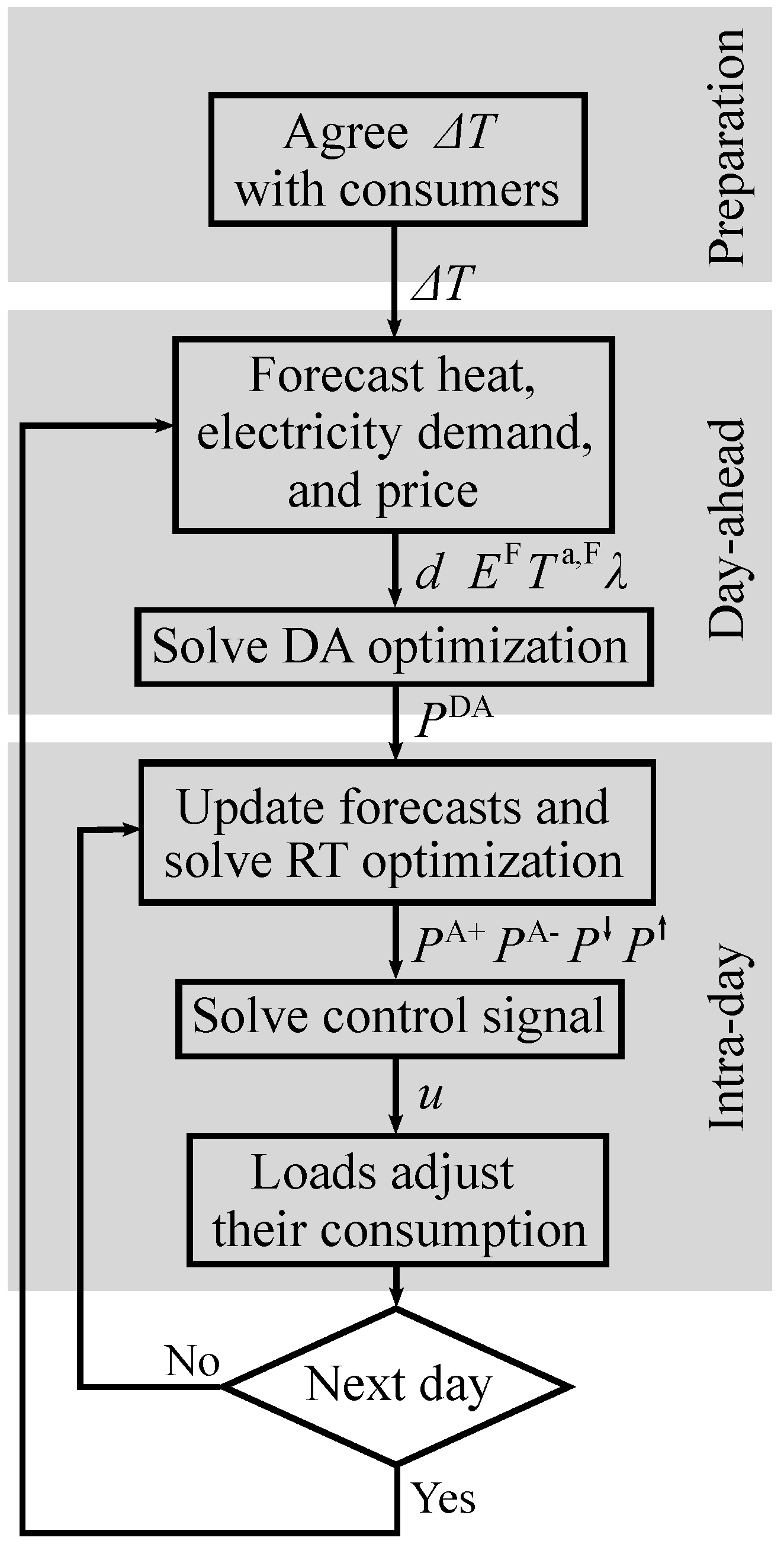
2.3. Control Strategy

The following introduces the stage by stage procedure of the control strategy, consisting of DA and RT actions. The procedure is also presented as a flowchart in Figure 1 where the symbols correspond to the notation used in the problem formulation in Section 3.2. Firstly, before the actual continuous operation, the aggregator makes contracts with the consumers and the allowed temperature band ($\Delta T$) is agreed upon. Furthermore, in order to help the aggregator implement the control strategy, the consumers can share information on their building type. Necessary communication infrastructure and controlling devices should also be installed.

In the DA stage, the aggregator procures its electricity demand from the DA market ($P^{\mathrm{DA}}$) as well as arbitrages between the DA market and BPM. The aggregator sets its orders so that the flexibility can be effectively utilized in the RT operation. This is performed by solving the self-scheduling problem of the aggregator at noon before the day of the delivery. For the scheduling, fixed electricity consumption (d), spot prices (λ), the heating power of the controlled buildings ($E^{\mathrm{F}}$), and the behavior of their indoor temperature ($T^{\mathrm{a},\mathrm{F}}$) need to be forecasted. In the RT stage, which takes place every hour, the aggregator defines regulating power bids to the BPM and possible consumption adjustments by solving the RT optimization. Next, the aggregator first adjusts its consumption ($P^{\mathrm{A}+}$, $P^{\mathrm{A}-}$) if necessary and performs the regulation ($P^{\uparrow }$, $P^{\downarrow }$) if the aggregator’s regulating bid is accepted by the TSO. The control for the adjustments and regulation is based on a generic control signal (u) broadcasted to controllable loads.

3. Problem Formulation

3.1. Local Optimization

The considered DESH loads desire reducing their electricity cost by scheduling consumption based on the electricity spot price. DESH is a heating process, which utilizes resistive heating with radiators located in the rooms of the building to convert electricity into heat. The conversion is typically done with high efficiency. Therefore, it is assumed that all the electricity drawn from the grid is converted to heating energy. The loads are assumed to have the thermal model of their building, which gives them the relationship between consumption and indoor temperature. Furthermore, they are able to predict the necessary input variables (temperature, solar radiation, heat gains, fixed electricity demand), but the forecasting is not considered here. The loads should also have the required intelligence to react to the centralized control signals explained in the next section.

The local optimization problem is a rolling horizon procedure, i.e., the optimization is updated every time step (hour) based on recent measurements and updated forecasts, and only the optimized action for the next time step is implemented. The local optimization problem is formulated as follows:

$$\min \sum _{k=1}^K{\lambda }_k·E_k,$$

(1)

subject to

$$A1·T_k^{\mathrm{a}}-T_{k-1}^{\mathrm{a}}-A2·T_k^{\mathrm{m}}=A3·E_k+A{4}_k\forall k,$$

(2)

$$-B1·T_k^{\mathrm{a}}+B2·T_k^{\mathrm{m}}-T_{k-1}^{\mathrm{m}}=B{3}_k\forall k,$$

(3)

$$T^{\mathrm{set}}-\Delta T^{\mathrm{L}}\le T_k^{\mathrm{a}}\le T^{\mathrm{set}}+\Delta T^{\mathrm{L}}\forall k,$$

(4)

$$E_k\le \overline{E}\forall k,$$

(5)

$$\frac{1}{K^{\mathrm{b}}}\sum _{k=K^{\mathrm{b}}·(l-1)+1}^{K^{\mathrm{b}}·l}{T}_k^{\mathrm{a}}\ge T^{\mathrm{set}}\forall l,$$

(6)

where the decision variables are E, $T^{\mathrm{a}}$, and $T^{\mathrm{m}}$.

The objective function (1) is to minimize the heating cost over a time horizon. In the objective, k is the time step, K is the length of the optimization period, λ is the electricity spot price, and E is the heating power. Constraints (2) and (3) model the evolution of the indoor ($T^{\mathrm{a}}$) and the building mass ($T^{\mathrm{m}}$) temperature, respectively. These constraints represent a two-capacity building thermal model capturing the thermal dynamics of a detached house [14]. Parameters $A1$–$A4$ and $B1$–$B3$ are obtained by discretizing the continuous dynamics as done in [15]. The indoor temperature is bounded by Equation (4), i.e., the temperature is allowed to deviate $\Delta T^{\mathrm{L}}$ from the indoor temperature set-point ($T^{\mathrm{set}}$). By giving a high value for $\Delta T^{\mathrm{L}}$, a consumer is able to increase the amount of heating load flexibility available for the optimization, and thus reduce the heating cost. The maximum heating power ($\overline{E}$) is forced by the constraint (5). Equation (6) forces the mean indoor temperature over $K^{\mathrm{b}}$ time steps to be greater than equal to the set-point temperature. This constraint ensures that the optimization maintains the mean indoor temperature close to the set-point value, which improves the consumer comfort. Otherwise, the optimization would simply reduce the cost by keeping the temperature at the minimum allowed level. In Equation (6), l is the index of the averaging block. From now on, the heating power E and the constraints (2)–(5) are given shorter expression $E_k^i=f(T_k^{\mathrm{a},\mathrm{i}},T_k^{\mathrm{m},\mathrm{i}},{\theta }^i)$ where θ defines a set of parameters, i.e., ${\theta }^i=\{A{1}^i,A{2}^i,A{3}^i,A{4}_k^i,B{1}^i,B{2}^i,B{3}_k^i,\Delta T^{\mathrm{L}},T^{\mathrm{set}},\overline{E}\}$.

3.2. Aggregators’ Decision-Making

Day-ahead optimization: In the DA market, the aggregator’s objective is to maximize its profit by defining optimal procured volumes while considering the available flexibility. The problem is formulated as a two-stage stochastic linear program [16], where the hourly DA procurements are the first stage (here and now) variables, and up/downregulation and positive/negative load adjustments are the key second stage (wait and see) variables. After the first stage decisions have been made, they become fixed and the second stage decisions are made for each scenario. The scenarios are used to model the uncertainly the aggregator faces in the DA stage. In this study, we assume that regulating prices and fixed electricity demand are uncertain, whereas the spot prices are assumed to be known. For simplicity, we also assume that the partial activation of the regulating power bids is not possible.

Note that the two-stage definition assumes that, in the second stage, information for the whole optimization period is available and decisions are made for this period. In practice, the decisions (regulating bids and adjustments) should be updated continuously based on actual realized regulation and consumption. We tackle this problem with the RT optimization, which is introduced in the next section. The DA optimization problem is

$$\begin{array}{cc}\hfill \max & \sum _{s=1}^S{\rho }_s\sum _{k=1}^K((m+{\lambda }_k)·P_{k,s}^{\mathrm{R}}-{\lambda }_k·P_k^{\mathrm{DA}}\hfill \\ & -(m+{\lambda }_k)·\Delta E_{k,s}^{+}+({\lambda }_{k,s}^{\uparrow }·P_{k,s}^{\uparrow }-{\lambda }_{k,s}^{\downarrow }·P_{k,s}^{\downarrow })\hfill \\ & +({\beta }^{+}·{\lambda }_{k,s}^{\mathrm{S}+}·P_{k,s}^{\mathrm{S}+}-{\beta }^{-}·{\lambda }_{k,s}^{\mathrm{S}-}·P_{k,s}^{\mathrm{S}-})),\hfill \end{array}$$

(7)

subject to

$$P_k^{\mathrm{DA}}-P_{k,s}^{\mathrm{R}}=P_{k,s}^{\mathrm{S}+}-P_{k,s}^{\mathrm{S}-}+P_{k,s}^{\uparrow }-P_{k,s}^{\downarrow }\forall k,s,$$

(8)

$$P_{k,s}^{\mathrm{R}}=d_{k,s}+E_{k,s}^{\mathrm{R}}\forall k,s,$$

(9)

$$\Delta E_{k,s}^{+}\ge E_{k,s}^{\mathrm{R}}-E_k^{\mathrm{F}}\forall k,s,$$

(10)

$$P_{k,s}^{\uparrow }\le \overline{E}·H_{k,s}^{\uparrow },P_{k,s}^{\downarrow }\le \overline{E}·H_{k,s}^{\downarrow }\forall k,s,$$

(11)

$$P_{k,s}^{\mathrm{A}+}\le \overline{E},P_{k,s}^{\mathrm{A}-}\le \overline{E}\forall k,s,$$

(12)

$$E_{k,s}^{\mathrm{A}}=E_k^{\mathrm{F}}+P_{k,s}^{\mathrm{A}+}-P_{k,s}^{\mathrm{A}-}\forall k,s,$$

(13)

$$E_{k,s}^{\mathrm{A}}=f(T_{k,s}^{\mathrm{a},\mathrm{A}},T_{k,s}^{\mathrm{m},\mathrm{A}},{\theta }^A)\forall k,s,$$

(14)

$$-\Delta T\le T_{k,s}^{\mathrm{a},\mathrm{A}}-T_k^{\mathrm{a},\mathrm{F}}\le \Delta T\forall k,s,$$

(15)

$$E_{k,s}^{\mathrm{R}}=E_k^{\mathrm{F}}+P_{k,s}^{\mathrm{A}+}-P_{k,s}^{\mathrm{A}-}+P_{k,s}^{\downarrow }-P_{k,s}^{\uparrow }\forall k,s,$$

(16)

$$E_{k,s}^{\mathrm{R}}=f(T_{k,s}^{\mathrm{a},\mathrm{R}},T_{k,s}^{\mathrm{m},\mathrm{R}},{\theta }^R)\forall k,s,$$

(17)

$$-\Delta T\le T_{k,s}^{\mathrm{a},\mathrm{R}}-T_k^{\mathrm{a},\mathrm{F}}\le \Delta T\forall k,s,$$

(18)

where the decision variables are $P^{\mathrm{R}}$, $P^{\mathrm{DA}}$, $\Delta E^{+}$, $P^{\uparrow }$, $P^{\downarrow }$, $P^{\mathrm{S}+}$, $P^{\mathrm{S}-}$, $P^{\mathrm{A}+}$, $P^{\mathrm{A}-}$, $E^{\mathrm{R}}$, $E^{\mathrm{A}}$, $T^{\mathrm{a},\mathrm{A}}$, $T^{\mathrm{m},\mathrm{A}}$, $T^{\mathrm{a},\mathrm{R}}$, and $T^{\mathrm{m},\mathrm{R}}$.

The objective function (7) consists of selling electricity to the consumers (the first term in the summation), procuring electricity from the DA market (the second term), evaluated cost to the consumers due to the control (the third term), trading in the BPM (the fourth and fifth terms), and the selling and procurement of imbalance power during the settlement process (the sixth and seventh terms). In the first row of the objective function, s is the scenario index, S is the number of scenarios used to model the uncertainties, k is the time step index, and K is the length of the optimization period. Thus, the optimization is solved over S scenarios and K time steps. Since every scenario is multiplied by its probability ρ, the objective function is to maximize the expected value of the aggregator’s profit for the following day. Furthermore, in the objective, m is the margin consumers pay in addition to the spot price λ. In the last row of the objective, weighting factors ${\beta }^{+}$ and ${\beta }^{-}$ are introduced to ensure that energy trading occurs in the DA market rather than via imbalance settlement if the spot and imbalance prices (${\lambda }^{\mathrm{S}+}$ or ${\lambda }^{\mathrm{S}-}$) are equal.

Constraint (8) defines the imbalance between the DA procurement ($P^{\mathrm{DA}}$) and the RT consumption ($P^{\mathrm{R}}$). It is used to solve the required positive ($P^{\mathrm{S}+}$) and negative ($P^{\mathrm{S}-}$) imbalance powers for every hour and scenario. Furthermore, in constraint (8), $P^{\uparrow }$ and $P^{\downarrow }$ are the up and downregulating powers, respectively. They are assumed to be equal to the bids offered to the BPM since partial activations are not allowed in this study. Equation (9) gives the RT consumption that is a sum of fixed electricity consumption (d) and the real-time heating power ($E^{\mathrm{R}}$). An evaluated increase in consumption ($\Delta E^{+}$) due to the control is forced by Equation (10), where $E^{\mathrm{F}}$ is the heating load forecast. Note that without $\Delta E^{+}$, the aggregator could profit by increasing consumption instead of using the flexibility effectively. Constraints (11) and (12) bound the regulating powers bids and the positive ($P^{\mathrm{A}+}$) and negative ($P^{\mathrm{A}-}$) adjustment powers, respectively. In constraint (11), $H^{\uparrow }$ and $H^{\downarrow }$ are predefined binary parameters, which get the value one if an hour is up (down)regulated, and zero otherwise. That is, regulation can only be provided when a regulating price scenario indicates that TSO activates regulating power. We assume that an hour can be either down or upregulated but not both.

At the beginning of the delivery hour, the aggregator first adjusts the consumption with $P^{\mathrm{A}+}$ or $P^{\mathrm{A}-}$, which is defined by Equations (13)–(15). The adjusted heating power ($E^{\mathrm{A}}$) given in Equation (13) is a sum of the forecasted heating load and the positive and negative adjustments. Equation (14) contains the heating load model and Equation (15) sets the allowed indoor temperature band for the control. The constraints (14) and (15) principally define the possible changes in the indoor temperature due to the adjustments. Similarly, Equations (16)–(18) define the consumption if the aggregator’s regulation bid is activated. Note that the adjustments influence Equation (16), as they are implemented before the regulation. The resulting RT heating power is the same that affects the RT consumption in Equation (9) and the evaluated increase in consumption in Equation (10).

Real-time optimization: The purpose of the RT optimization is to update the aggregator’s decisions based on the recent measurements of consumption and indoor temperature and updated forecasts. By utilizing the optimization, flexibility resources can be reallocated between the BPM and imbalance power. As a result, the optimization provides regulating power bids and the adjustments of the heating load for the coming hour. Updating the decisions by using up to date information is crucial because of the local optimization, which employs the rolling horizon procedure. This is to say, every centralized control action leads to changes in the future load of the consumers.

The formulation of the RT problem closely follows the second stage of the DA optimization when the DA procurement has already been fixed. The main differences between the DA and RT formulations are the fixed DA procurement, i.e., $P^{\mathrm{DA}}$ is a parameter instead of a variable, and updated heating load forecast and scenarios. However, in this study, we assume that the consumption and regulating prices can be perfectly forecasted at the RT stage. The RT formulation is

$$\begin{array}{cc}\hfill \max & \sum _{s=1}^S{\rho }_s\sum _{k=1}^K((m+{\lambda }_k)·P_{k,s}^{\mathrm{R}}\hfill \\ & -(m+{\lambda }_k)·\Delta E_{k,s}^{+}+({\lambda }_{k,s}^{\uparrow }·P_{k,s}^{\uparrow }-{\lambda }_{k,s}^{\downarrow }·P_{k,s}^{\downarrow })\hfill \\ & +({\beta }^{+}·{\lambda }_{k,s}^{\mathrm{S}+}·P_{k,s}^{\mathrm{S}+}-{\beta }^{-}·{\lambda }_{k,s}^{\mathrm{S}-}·P_{k,s}^{\mathrm{S}-})),\hfill \end{array}$$

(19)

subject to Equations (8)–(18).

Control: After the RT optimization, the aggregator needs to control the loads so that the consumption can be adjusted and possibly regulated if the TSO requests regulating power. For the RT control, we propose a generic control signal broadcasted to the loads. The signal is defined as the ratio of the desired heating power to the maximum heating power. Thus, for example, an adjustment communicated to the load is $u=E^{\mathrm{A}}/\overline{E}$. When the loads receive the signal, they first solve the maximum and minimum powers based on the allowed temperature band. Then, the performed control action is either the requested power ($E=u·\overline{E}$) or it is limited by the possible changes in the indoor temperature.

4. Simulations

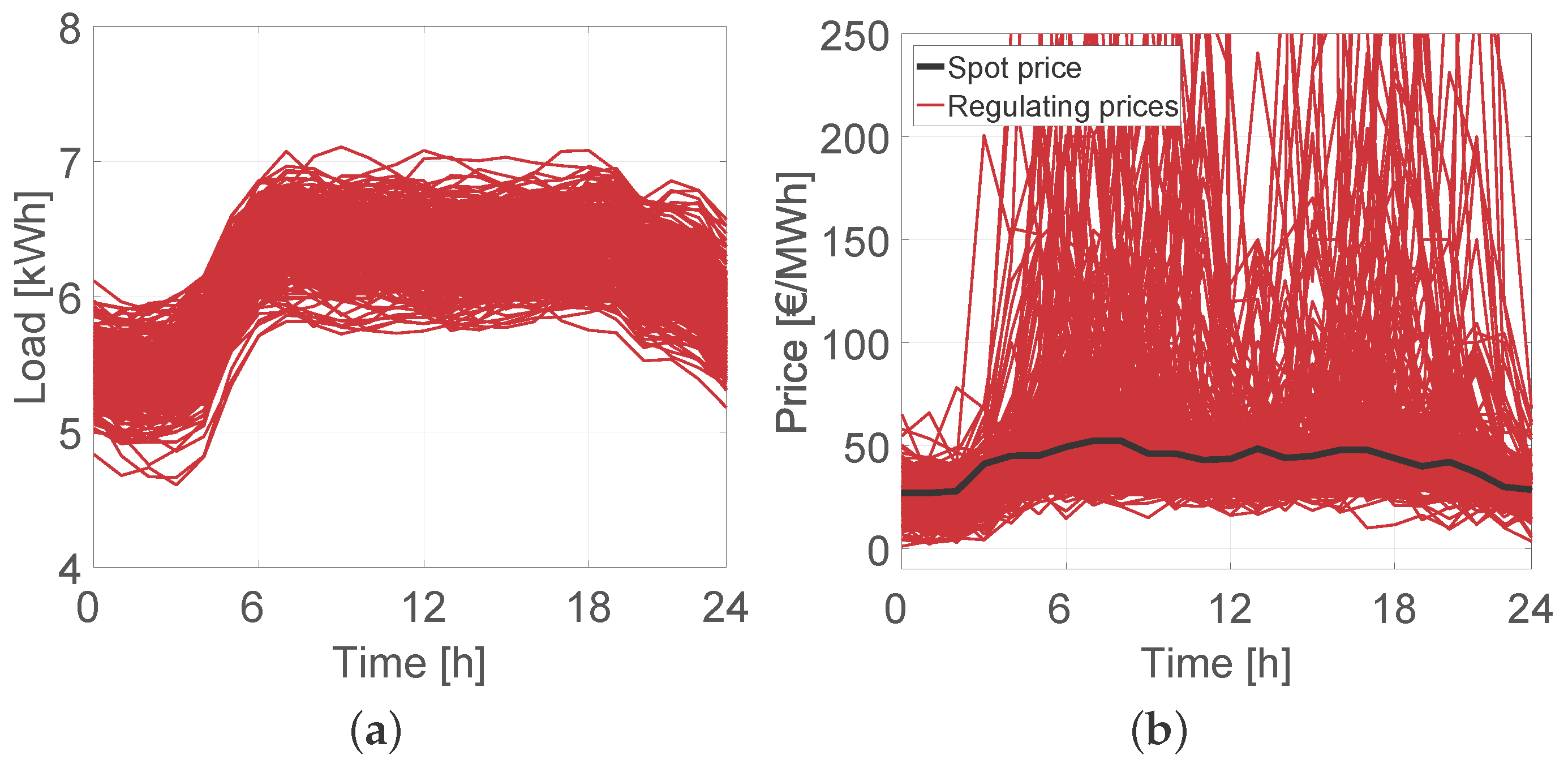
4.1. Simulation Setup

The simulations aim to illustrate the operation of the control strategy and show its benefits. The core of the simulation model is formed by the studied building stock, the generation of price and load scenarios, and the employed data, which are described in the following. The building stock consists of 12 representative Finnish building types comprising light weight, medium weight, and massive structure buildings constructed in different decades (1960–1979, 1980–1999, 2000–2009, 2010–2013). The parameter values for each building type are solved based on the guidelines in [17] or the Finnish 2010 building code [18]. More detailed description on some of studied building types can be found in [19]. The buildings are assumed to be located in the Uusimaa region in Southern Finland, and, therefore, we use outdoor temperature and solar radiation data measured in Helsinki in 2012 as inputs. The effect of internal heat gains (lighting, appliances, occupants) is also considered. The appearance of the studied building types varies in Uusimaa [20]. Thus, when analyzing the results, the heat demands of the 12 simulated types are weighted based on the actual number of these houses and their floor areas in Uusimaa. The same scaling factors are also employed to form an aggregated heating load model for the centralized optimization. For clarification, the 12 building types are simulated and the aggregated model is used in the DA and RT optimizations.

To characterize hourly fixed electricity consumption and regulating prices for scenario generation, two separate dynamic regression models are implemented. The approach for consumption is based on the one presented in [21] so that the dependent variable (consumption) is explained here by its lagged values, outdoor temperature, day length, and day type. In the case of the regulating price model, the lagged values of regulating prices and DA market prices are used as explanatory variables. However, for the actual model fitting, the data transformation is first performed, which forces the data to follow Gaussian distribution, as in [22]. After time series have been generated with the model, they are transformed back to follow the original distribution of the price data. The price and consumption data are from references [10,13].

We use Wednesday the 14th of March in 2012, a typical weekday with nearly zero outdoor temperature, as an illustrative day. One thousand scenarios with even probability (1/1000) are generated for load and prices, after which the number is reduced to 300 for the DA optimization by employing scenario reduction [16]. For the actual hourly simulation, we generate a new set of 300 scenarios, which are shown in Figure 2. The scenario reduction is performed to relieve the computational burden, which increases along with the number of scenarios. The number 300 has been selected as a trade-off between simulation time and the stability of the solution. The solution stability is to say that the results remain somewhat the same despite the selected set of simulated scenarios.

The DA optimization problem is solved with a 48 h horizon (the studied day and a one day look-ahead), whereas the RT problem uses only a two hour horizon and perfect forecasts for prices and fixed load. Weighting factor values of 0.999 and 1.001 were set for ${\beta }^{+}$ and ${\beta }^{-}$, respectively, and a margin of 1 €/MWh is used in the consumer tariff. In the local optimization problem, we assume that the loads use a 24 h horizon divided into two averaging blocks. The loads can vary the indoor temperature between 19 and 23 °C, while the set-point is 21 °C. The allowed temperature band for the aggregator is 1 °C. The simulations are implemented in MathWorks MATLAB R2016a (MathWorks, Natick, MA, USA), which further calls GAMS and CPLEX to solve the optimizations. The following three cases are simulated and presented:

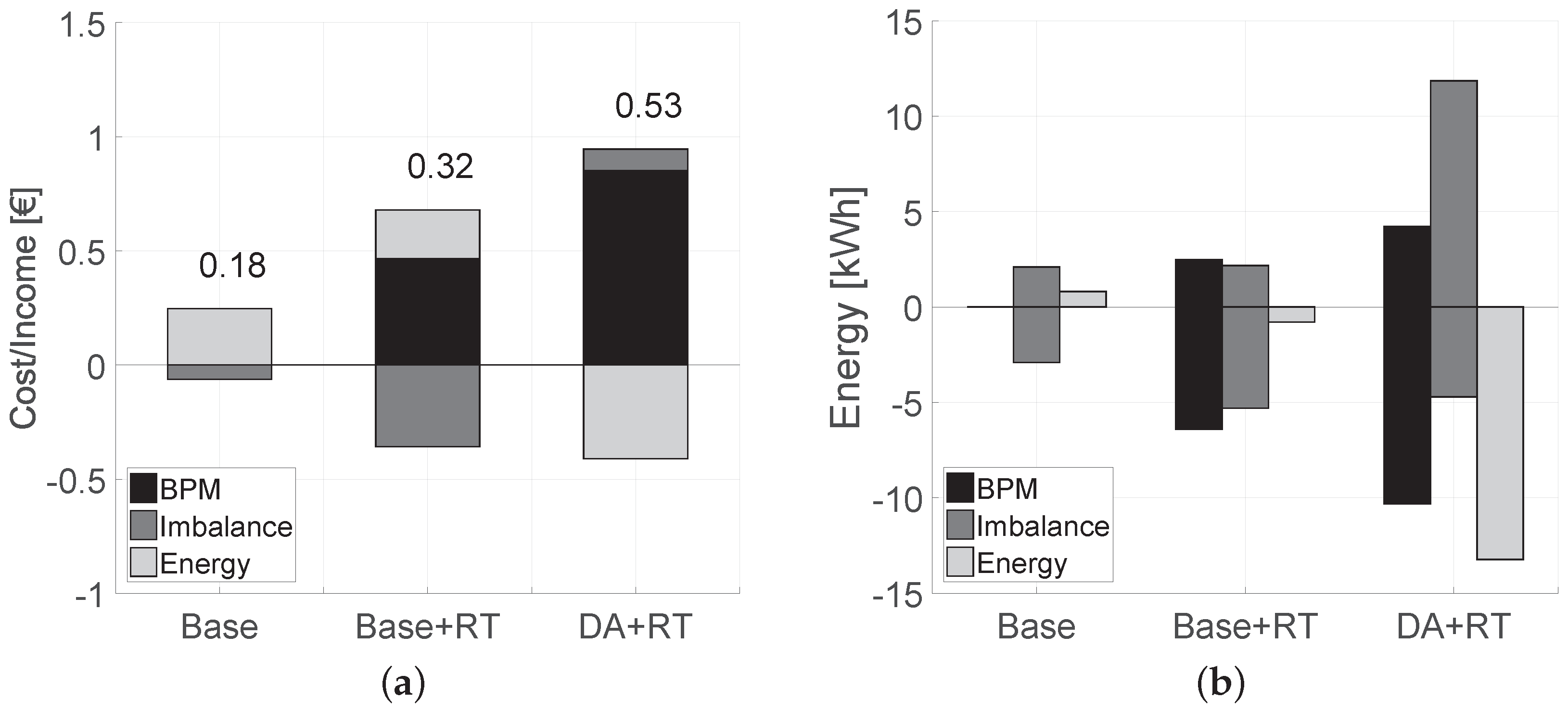
• Base: Loads optimize locally but they cannot be centrally controlled. However, the aggregator is able to bid in the DA market but without the heating load flexibility.
• Base+RT: RT optimization and control are possible but the flexibility is not considered in the DA optimization.
• DA+RT: The DA optimization is solved with the heating load flexibility and the operation is updated by solving the RT optimization. The aggregator is also able to control the loads.

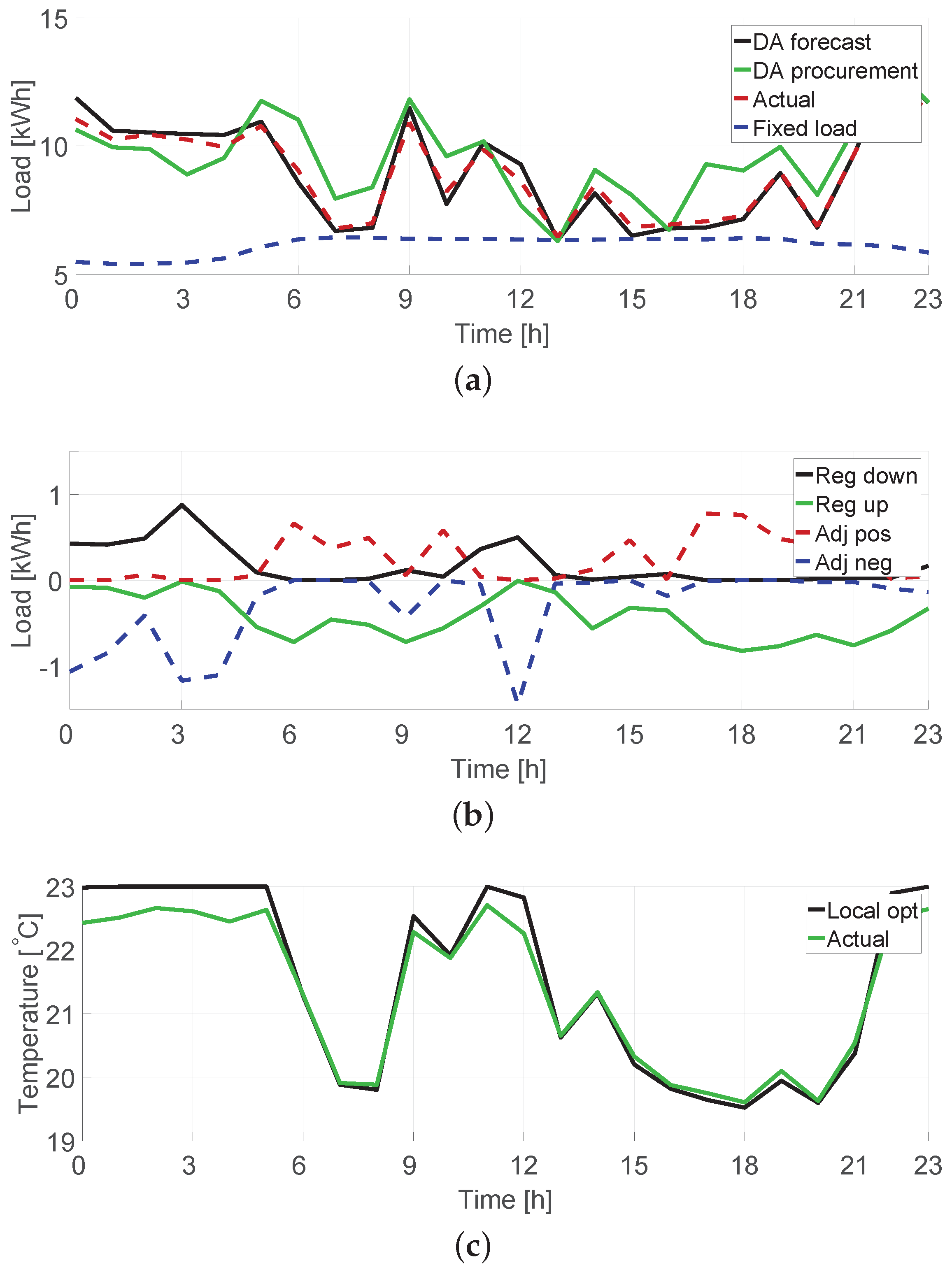
For each of the cases, the DA optimization is first solved with the reduced set of scenarios to provide the DA procurement, after which the new set of scenarios is simulated hour by hour (300 days) in order to test the RT optimization and control. The results are presented as average values over the scenarios.

4.2. Results

The basic operation of the proposed strategy is illustrated in Figure 3, which shows average hourly values for DA forecast and procurement, actual load (simulated heating load plus fixed electricity consumption) and fixed electricity consumption, regulation and adjustments, and the indoor temperature for the case DA+RT. The loads are presented in Figure 3a, where the black line is the DA forecast, the green line is the DA procurement, the dashed red line the actual load, and the dashed blue line is the fixed electricity consumption. The pattern of optimized heating load is clearly visualized by the black line: the consumption is increased at night and decreased during the day time. The DA procurement follows these patterns, but it can be seen that excess electricity is procured for the morning and evening peak hours, whereas the procurement is less than the forecast at night. The actual consumption, on the other hand, is close to the forecasted load.

The reason for this behavior can be found in Figure 3b, which depicts up and downregulation (black and green lines) as well as positive and negative adjustments (dashed red and blue lines). It can be seen how negative adjustment and downregulation occur mainly at night, i.e., owing to the deficit DA procurement, the heating power can be reduced and downregulation provided to the BPM. On the other hand, the heating power is increased in the morning and evening when excess electricity was procured. As seen in Figure 2b, the occurrence of price spikes in the upregulating price slightly increase in the morning and evening, which is also when the most upregulation is provided by the aggregator (green line in Figure 3b). Finally, the actual indoor temperature is shown in Figure 3c together with the locally optimized indoor temperature profile (this is the target temperature before the aggregator controls the loads). It can be seen in the figure that the temperature remains within the allowed temperature band.

Next, we compare the different studied cases in terms of the aggregator’s profit and the traded energies and the regulating and imbalance powers in Figure 4. Figure 4a reveals the profit in different cases and shows its components: trading in the BPM, selling/buying of imbalance power, and energy trading (selling minus DA procurement). In the Base case, the aggregator aims to maximize its expected energy trading income while avoiding high imbalance costs. The aggregator is able to profit from energy selling since the consumers pay the margin in addition to the spot price. In the case Base+RT, the DA procurement remains the same as in the Base case, but now the aggregator can participate in the BPM and adjust the consumption in real-time. This basically results in the selling of upregulation and increased profit. However, the imbalance cost also increases. When the possibility to control the loads is considered in the DA optimization (case DA+RT), the profit further increases. Now, the aggregator is able to arbitrage between the DA market and BPM, which increases its income in the BPM. We also observed the same behavior in Figure 3: the aggregator procures excess electricity in the morning and evening, enabling the selling of upregulation, and procured less electricity at night time in the DA market, which enabled it to buy downregulation at the downregulating price (less than or equal to the spot price). Furthermore, after including the flexibility in the DA optimization, the imbalance costs are better managed compared to the Base+RT case. The arbitraging and decreased imbalance cost, however, results in negative energy trading due to increased DA procurement compared to the other cases.

Figure 4b summarizes the daily average energies traded in the BPM (positive is down and negative upregulation), positive and negative imbalance powers, and energy trading in the DA market. The figure shows that more up and downregulation is provided if the flexibility is considered in the DA optimization compared to the Base+RT case. However, this increases the need for positive imbalance power. It can also be seen that the aggregator procures close to the expected demand from the DA market (energy trading close to zero) in the Base and Base+RT cases. In the case of DA+RT, the consumption is less than the procurement instead.

Even though the proposed control strategy allows the aggregator to profit, the cost to consumers may increase since their optimized profile is centrally altered. However, for the cases Base, Base+RT, and DA+RT, the consumer costs without any compensation from the aggregator are 2.70 €, 2.66 €, and 2.65 €, respectively. Therefore, the control has only a minor, but beneficial, influence on the consumer costs, which we owe to the formulation penalizing increased heating load consumption. Furthermore, a part of the aggregator’s profit is naturally paid to the controlled consumers via bonuses. As it can be seen in Figure 4a, the strategy enables the aggregator to approximately triple its profit from 0.18 € to 0.53 €. Thus, the aggregator becomes more profitable and the consumers are able to benefit from the increased profit via bonuses.

5. Conclusions

This paper proposed a control framework enabling an aggregator to centrally adjust cost minimizing loads. Such an ability protects the aggregator from possible price and demand forecast errors as well as allows the aggregator to participate in the BPM and gain extra profit. A part of the profit is paid to the consumers via bonuses. A central part of the strategy was the indoor temperature band, which dictates the flexibility available to the aggregator. The proposed control framework consisted of the DA and RT optimization problems, which can be employed to allocate the flexibility between the DA market, the BPM, and the imbalance power. Furthermore, the generic control signal was proposed for the activation of the demand-side flexibility.

Simulation studies were performed to showcase the operation of the strategy. In general, the strategy allowed the aggregator to increase its profit. It was also found that the aggregator would rather buy less from the DA market for the night hours in order to be able to procure the energy later in the BPM. On the other hand, particularly for the morning and evening hours, excess energy was procured in the DA market so that upregulation could be sold in the BPM. This is to say, the aggregator was able to reserve flexibility for real-time operation and it arbitraged between the markets to gain profit. Such behavior increased the required imbalance power but did not increase its cost.

References

1. Siano, P. Demand response and smart grids—A survey. Renew. Sustain. Energy Rev. 2014, 30, 461–478. [Google Scholar] [CrossRef]
2. Beaudin, M.; Zareipour, H. Home energy management systems: A review of modelling and complexity. Renew. Sustain. Energy Rev. 2015, 45, 318–335. [Google Scholar] [CrossRef]
3. Yang, S.; Zeng, D.; Ding, H.; Yao, J.; Wang, K.; Li, Y. Multi-objective demand response model considering the probabilistic characteristic of price elastic load. Energies 2016, 9, 80. [Google Scholar] [CrossRef]
4. Weckx, S.; D’Hulst, R.; Driesen, J. Primary and secondary frequency support by a multi-agent demand control system. IEEE Trans. Power Syst. 2015, 30, 1394–1404. [Google Scholar] [CrossRef]
5. Alahäivälä, A.; Ali, M.; Lehtonen, M.; Jokisalo, J. An intra-hour control strategy for aggregated electric storage space heating load. Int. J. Electr. Power Enery Syst. 2015, 73, 7–15. [Google Scholar] [CrossRef]
6. Sarker, M.R.; Ortega-Vazquez, M.A.; Kirschen, D.S. Optimal coordination and scheduling of demand response via monetary incentives. IEEE Trans. Smart Grid 2015, 6, 1341–1352. [Google Scholar] [CrossRef]
7. Fan, W.; Liu, N.; Zhang, J.; Lei, J. Online air-conditioning energy management under coalitional game framework in smart community. Energies 2016, 9, 689. [Google Scholar] [CrossRef]
8. Corradi, O.; Ochsenfeld, H.; Madsen, H.; Pinson, P. Controlling electricity consumption by forecasting its response to varying prices. IEEE Trans. Power Syst. 2013, 28, 421–429. [Google Scholar] [CrossRef]
9. Zugno, M.; Morales, J.M.; Pinson, P.; Madsen, H. A bilevel model for electricity retailers’ participation in a demand response market environment. Energy Econ. 2013, 36, 182–197. [Google Scholar] [CrossRef]
10. Nord Pool. Nord Pool Spot. Available online: www.nordpoolspot.com (accessed on 7 April 2016).
11. Finnish Energy. Consumption and Network Losses of Electricity. Available online: energia.fi/en/statistics-and-publications/electricity-statistics/electricity-consumption/consumption-and-network-l (accessed on 1 November 2016).
12. Fingrid Oyj. Balancing Power Market. Available online: www.fingrid.fi/en/electricity-market/reserves/acquiring/market/Pages/default.aspx (accessed on 1 November 2016).
13. Fingrid Oyj. Electricity Market and Balance Service. Available online: www.fingrid.fi/en (accessed on 7 April 2016).
14. Ali, M.; Safdarian, A.; Lehtonen, M. Demand response potential of residential HVAC loads considering users preferences. In Proceedings of the IEEE PES Innovative Smart Grid Technologies Europe, Istanbul, Turkey, 12–15 October 2014.
15. Alahäivälä, A.; Ekström, J.; Jokisalo, J.; Lehtonen, M. A framework for the assessment of electric heating load flexibility contribution to mitigate severe wind power ramp effects. Electr. Pow. Syst. Res. 2017, 142, 268–278. [Google Scholar] [CrossRef]
16. Conejo, A.J.; Carrión, M.; Morales, J.M. Decision Making Under Uncertainty in Electricity Markets; Springer: New York, NY, USA, 2010. [Google Scholar]
17. Ministry of the Environment. Decree for the Energy Certificate (176/2013). Available online: www.finlex.fi/data/sdliite/liite/6186.pdf (accessed on 7 April 2016). (In Finnish)
18. Ministry of the Environment. C3: Finnish Code of Building Regulations (Thermal Insulation in a Building); Ministry of the Environment: Helsinki, Finland, 2010. (In Finnish)
19. Alimohammadisagvand, B.; Alam, S.; Ali, M.; Degefa, M.; Jokisalo, J.; Sirén, K. Influence of energy demand response actions on thermal comfort and energy cost in electrically heated residential houses. Indoor Built Environ. 2015. [Google Scholar] [CrossRef]
20. Official Statistics of Finland (OSF). Electrically Heated Detached Houses by the Year of Construction and Construction Material in Finland; Official Statistics of Finland: Helsinki, Finland, 2013. [Google Scholar]
21. Koivisto, M.; Degefa, M.; Ali, M.; Ekström, J.; Millar, J.; Lehtonen, M. Statistical modeling of aggregated electricity consumption and distributed wind generation in distribution systems using AMR data. Electr. Power Syst. Res. 2015, 129, 217–226. [Google Scholar] [CrossRef]
22. Koivisto, M.; Seppänen, J.; Mellin, I.; Ekström, J.; Millar, J.; Mammarella, I.; Komppula, M.; Lehtonen, M. Wind speed modeling using a vector autoregressive process with a time-dependent intercept term. Int. J. Electr. Power Enery Syst. 2016, 77, 91–99. [Google Scholar] [CrossRef]
Figure 1. Flowchart of the control strategy. The notation correspond to the notation of day-ahead (DA) and real-time (RT) optimization problems.
Energies 09 00983 g001
Figure 2. (a) Generated scenarios for the fixed load; and (b) Generated scenarios for regulating prices.
Energies 09 00983 g002
Figure 3. Average time series illustrating the operation. (a) DA forecast, DA procurement, actual simulated consumption, and fixed load; (b) Activated regulation and adjustments; (c) Locally optimized indoor temperature and the temperature after control.
Energies 09 00983 g003
Figure 4. Daily values. (a) Stacked bar graph presenting the components of aggregator’s profit. Negative values are cost and positive income. The values above the bars are the daily profits; (b) Grouped bar graph presenting the amount of up/downregulation (up is negative value), positive/negative imbalance powers, and energy trading.
Energies 09 00983 g004