
A Co-Simulation Framework for Power System Analysis


Energy Efficiency Research Division, Korea Institute of Energy Research, 152 Gajeong-ro, Yuseong-gu, Daejeon 34129, Korea
*
Author to whom correspondence should be addressed.
Energies 2016, 9(3), 131; https://doi.org/10.3390/en9030131
Submission received: 16 November 2015
/
Revised: 5 February 2016
/
Accepted: 5 February 2016
/
Published: 25 February 2016
(This article belongs to the Special Issue Electric Power Systems Research)
Abstract
:Power system electromagnetic transient (EMT) simulation has been used to study the electromagnetic behavior of power system components. It generally comprises detailed models of the study area and an equivalent circuit which represents an external part of the study area. However, a detailed description of an external system that includes transmission or distribution system models is required to study the interaction among power system components because the number of high power converter based devices in a power grid have been increasing. Since detailed models of the system components are necessary to simulate a series of events such as cascading faults the computational burden of power system simulation has increased. Therefore a more effective and practical framework has been sought to handle this computational challenge. This paper proposes a co-simulation framework including a delay compensation algorithm to compensate the time delayed signals due to network segmentation and a fast and flexible simulation environment composed of non-real time power system EMT simulation on a general purpose computer with a multi core central processing unit (CPU), which is currently very popular owing to its performance. The proposed methods are applied to an AC/DC power system model.
1. Introduction
Since power electronic systems such as high voltage direct current (HVDC) and flexible alternating current transmission are widely used in power systems, the need for electromagnetic transient (EMT) studies to assess their effect on power systems has increased. Recently, the penetration level of distributed energy resources (DERs) such as photovoltaic, wind, fuel cell, has increased due to environmental issues and fossil fuel prices, which can result in uncertainties on both the supply and demand sides [1]. DERs use power electronics circuits to generate, convert and inject electric power into a distribution system. Therefore, an EMT simulation which includes both DERs and detailed power system component models is required to evaluate the effect of the increased uncertainties on a power grid and to develop appropriate countermeasures. However, to adequately simulate power systems using these detailed models, the integration time-step of the simulation must be sufficiently smaller than the time constant of the fastest EMT phenomena of the system. Because EMT simulation aims to solve both the nodal equations for the substituted network and the differential equations which describe the dynamic behavior of the detailed models [2,3], EMT simulation of a complex power system with a small fixed time-step would result in huge computational burden and would remarkably increase the computation time of the EMT simulation.
A high performance CPU can make the EMT simulation run faster. However, technical and economic constraints currently exist in terms of increasing the operating speed of CPUs. To overcome these constraints much research have been done on the simulation algorithms and techniques [4,5,6,7]. Most of these techniques are based on the fact that a power system can be divided into several subsystems and the subsystems can be simulated independently by the transmission line model (TLM) [8] which enables the decoupling of two subsystems by the wave propagation delay. This parallel simulation enables to distribute the computational load among the processing cores to more efficiently utilize the available computing power of a multi-core CPU. It is one of the co-simulation techniques which allows individual components to be simulated using different simulation tools which simultaneously execute and exchange information in a collaborative manner [9,10]. Unlike parallel processing [11,12], which divides a complex system into several subsystems and processes them in a single simulation system, co-simulation consists of several independent simulation programs and offers more simulation flexibility. The wave propagation delay which has been widely used to decouple two subsystems and allow each subsystem to be executed independently is the foundation of the co-simulation. However this time delay can be a bottleneck to enhance the overall accuracy and the stability of the co-simulation in some cases.
This paper proposes a co-simulation framework including a time-delay compensation algorithm which enables processing of time-consuming EMT simulation of complex power systems by two independent EMT simulations in a cooperative manner. The delay compensation method can enhance the accuracy and the stability of the EMT co-simulation and thus can alleviate the hardware and software limitations of the conventional EMT simulation on a general purpose personal computer. Unlike the message passing interface parallel programming, the proposed method can be implemented using commercial power system analysis software without modification of its source code. To evaluate the performance of the proposed method, examples of co-simulation of an AC/DC power system are presented and compared with the conventional simulation results.
2. EMT Co-Simulation Framework
The EMT co-simulation method generally comprises network partitioning, interfacing algorithm which integrates two decoupled subsystems. The network partitioning uses the reactive components, inductor or capacitor as transmission line to decouple two parts at the end of the line using the wave propagation delay. If a transmission line length is 15 km its propagation delay is about 50 μs. Therefore two subsystems which is connected with a 15 km long transmission line cannot see the change of the other side in 50 μs thus can be simulated independently. However the delay will be decreased proportional to the interface line length thus the time-step of the simulation should be decreased. The decreased time-step will increase the number of computation and thus total computation time.
The total simulation time depends on both the computation and data communication. The computation time for each subsystem is proportional to the size and complexity of the power systems being simulated. Because each pre-defined simulation sequence may not be completed before the data exchange among computing nodes in a non-real time simulation environment, some of the nodes idly wait for the data exchange, even in a parallel protocol, unless a prediction algorithm is applied [13]. Therefore, the need to reduce the computation time of each subsystem simulation and the total communication time between simulations is necessary to accelerate the co-simulation.
2.1. Network Partitioning
A network can be split into small subsystems by a network partitioning algorithm. The number of subsystems should be determined to minimize both communications between subsystems and the idle time of the simulation process since small subsystems take less time to solve system equations however increases the communication cost [14].
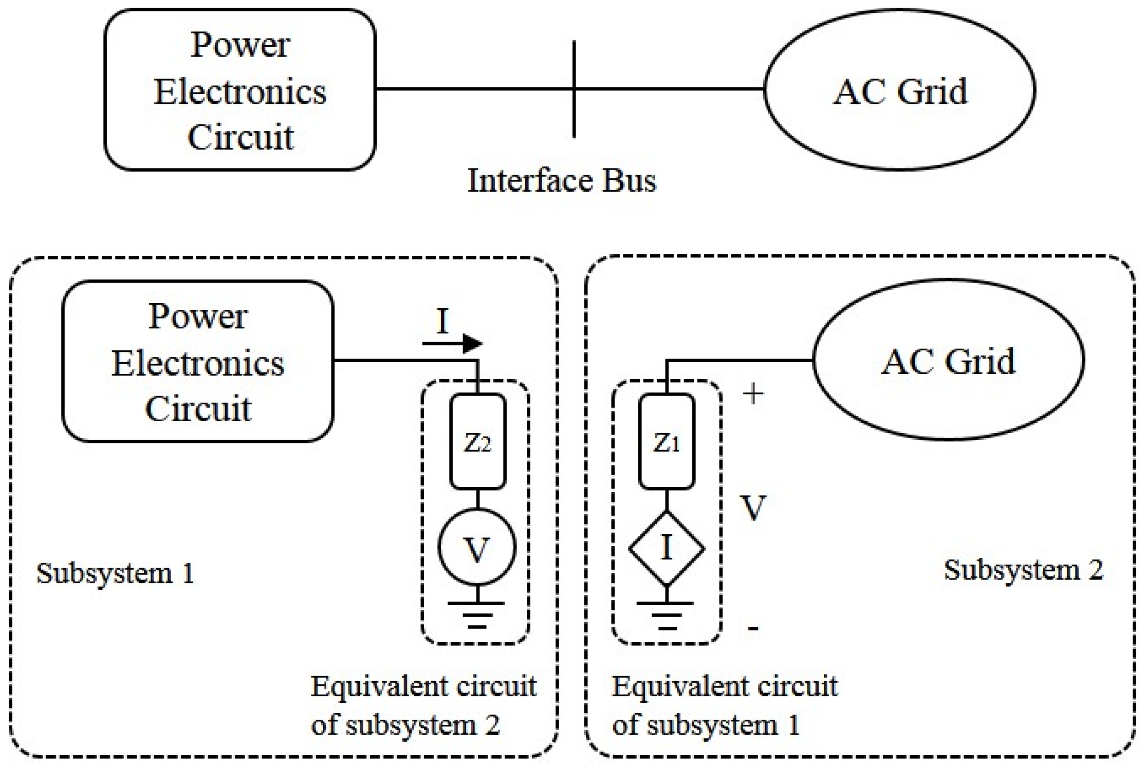
Since a power electronics circuit is generally very complex and has several high frequency switching devices which require high computational power to be simulated a power system which has power electronics circuits may be split into two subsystems at the interconnection point, as shown in Figure 1. The interconnection point will be the interface of the subsystems. The AC grid can be further partitioned to adjust the balance of the computational load of co-simulation. This characteristic-base partitioning can easily embrace the multi-time-step simulation algorithm and its loosely coupled connection increases reusability of a simulation model. It can also be easily applied in a commercial off-the-shelf graphical user interface (GUI)-based power system simulation program. This approach requires equivalent circuits that can fully simulate the dynamic behavior of each subsystem because the simulation accuracy depends on these equivalent circuits [15,16]. Power frequency based R-L-C networks have been used for the equivalent circuits. However, more sophisticated models are required if waveform distortion or phase imbalance occurs at the interface bus [17]. The circuits are modeled as frequency dependent using vector fitting [18,19].
2.2. Interfacing
Much research on the interfacing method has been carried out for power hardware testing in simulation environments [20,21,22]. Two major approaches to split a network into subsystems are the travelling wave model [23], and the insertion of time-step delays [24].
The subsystems have been split using travelling wave transmission lines in order to decouple the subsystems and solve them independently. The simulation time-step should be set to an integer fraction of the propagation delay of a travelling wave thus partitioning small power systems which have no long transmission lines such as microgrids, industrial power systems, shipboard power systems with the propagation delay using the travelling wave model requires very short simulation time-step to decouple the subsystems. The short time-step naturally increases the number of computation and communication thus makes EMT simulation very slow.
The time-step delay insertion method adds artificial delay to decouple the subsystems. The artificial delay is usually implemented with a stubline which length has one simulation time-step for the wave propagation delay. This artificial delay is quite useful especially to split the small size power systems, however, it may accumulate phase drifts and make simulation inaccurate and unstable [14].
Interface algorithm defines how two decoupled subsystems are interconnected. In this paper ideal transformer model (ITM) [25] is adopted for interfacing subsystems. It generates accurate result and is easy to set up. The measured voltage and current values at the interface of the subsystems are to be exchanged between the subsystems through their equivalent circuits as in Figure 1.
An ideal communication protocol for subsystem interfacing can make co-simulation continuously run without any idle time between the simulation time-steps. To minimize the idle time of the co-simulation of power systems, the parallel protocol proposed in [26] is adopted. It is reasonable to initiate the interfacing sequence with transferring the voltage values first which is 1 in Figure 2 since all the power electronics systems start to operate after being fed enough voltage from a power grid except black starting.
In a serial protocol, only one simulation time segment runs at each time instance while the other one stays idle. However, using the parallel interface protocol shown in Figure 2, both simulation segments, labeled as 4, can be concurrently run, thus minimizing the idle time. To eliminate the idle time, two distinct simulation sequences, labeled as 4, must be simultaneously executed. However, achieving this simultaneous simulation is very difficult with the network partitioning in a GUI based simulation environment. In practice, in an EMT-to-EMT co-simulation environment, the total idle time can be slightly longer than the ideal case.
The actual data transfers between two subsystems are carried by a pipe which is one of the inter-process communication (IPC) mechanisms as shown in Figure 3. It is an information conduit and allows a process to read and write from its end. It can be used to transfer data between unrelated processes over a network. It can provide simple programming interfaces since the synchronization is built into the pipe mechanism itself.
2.3. Time-Step Delay Error
Network partitioning inherently introduces time delays in the network. The parallel interface protocol shown in Figure 2 introduces a time-step delay to the lower side of the co-simulation, which is usually intended for the grid. The simulation time-step which is conventionally set to 50 to 100 μs requires 15 to 30 km length transmission line. Without a proper interface transmission line the artificial delay which is imposed by the simulation time-step causes the phase error to the sinusoidal signal at the interface and should be compensated to maintain the accuracy of the simulation.
A differential equation, namely Equation (1), which describes the dynamic behavior of the power system components, can be converted into a simple algebraic equation, i.e., Equation (3), by the trapezoidal rule:
Each side of the co-simulation processes shown in Figure 2 can be described by the following equations. Equations (5) and (6) describe the upper side shown in Figure 2, whereas Equations (7) and (8) represent the lower side. The ubci(n) term in Equation (9) represents the ith interface value, which is exchanged between the subsystems. The errors which result from the delay in one subsystem would influence the simulation result of the other subsystem:
The error due to the delay in the control signals is usually negligible. However, it can have a strong effect on the network solutions because the calculation of the power flow on the interface of the subsystems may be different at both sides of the subsystems due to the delay. In the case of a power flow with large effect on the grid, the errors cannot be neglected. The error in the delay should be properly compensated to enhance the accuracy of the entire EMT co-simulation. The error due to the delay varies with the size of the integration time-step and the frequency of the signals to be exchanged.
2.4. Data Prediction by Extrapolation
The delay error can be compensated using two time-step time shifts. The time shift of a signal can be obtained by predicting future data. Extrapolation is the process of estimating new data points outside a discrete set of known data points. Fundamentally, it is the same as the interpolation process, which constructs new points among known points. The interpolation algorithm can be applied as is to the estimation using the extended xi range outside the known values. However, the interval should be kept as small as possible to maintain the estimation quality.
The most straightforward extrapolation method is the linear extrapolation, as expressed in Equation (11). It creates a tangent line at the end of the known data and extends it beyond that limit. It assumes that any slopes between two adjacent points are fixed, and the extrapolation interval is sufficiently small to satisfy the assumption because the error of the linear method is proportional to the square of the interval, i.e., O(h2). As expressed in Equation (11), linear extrapolation assumes that the future data yk + 1 are on the line which passes two adjacent past data yk − 1 and yk. The algorithm is straightforward, and the computational load is minimal. However, the assumption can fail with high frequency signal components in the EMT simulation; thus, the integration time-step should be limited to be short enough to maintain the accuracy of the co-simulation. This process results in the increase in the total number of computations and thus the computational load:
A polynomial based algorithm shows much better performance than the linear method, as shown in Figure 4. The cubic spline method, whose error is expressed as O(h4), can reduce the interval to 13% compared with the linear method at the same level of summation of squared error (SSE).
The fundamental principle of the cubic spline method is to find a piecewise function which fits a given data set. The piecewise function consists of n − 2 third-degree polynomial, as expressed in Equation (12), with n points. The second derivative of each polynomial may be set to zero at the endpoints to satisfy the natural cubic spline condition. With the natural cubic spline condition Sk(x) can be arranged as a tridiagonal system which is easy to solve to obtain the polynomial coefficients:
The extrapolation would provide a minimum error using two properly selected parameters such as the number of given data points and the extrapolation interval. The interval should be set to a small value because it is directly related to the error of the cubic spline method. The iterative extrapolation based on a sliding window, as shown in Figure 5, can in effect reduce half of the interval to estimate the two step forward value.
The other factor which affects the accuracy of the cubic spline extrapolation is the length of the data window because the extrapolation estimates the unknown values using the given data set. Figure 6 shows the SSEs of the cubic spline method with different numbers of data points to extrapolate a one-cycle sinusoidal signal. Given five data points, the sliding window method gives a minimum error in the two step forward estimation of the sinusoidal function.
2.5. Discontinuity Detection
Discontinuities such as voltage drops due to a line fault are common phenomena in power systems. Accurately predicting such discontinuities using a series of discrete data to compensate the delay is quite difficult. Prediction using a limited number of known points tends to induce numerical spikes or oscillation. The spline method is more vulnerable to discontinuity, and its effect would appear more severe than the linear method because it uses derivatives to solve the tridiagonal system equation. The magnitude of this phenomenon is proportional to that of the derivative at the discontinuity.
Although an oscillation would disappear within a few steps, it may affect the accuracy of the co-simulation. To avoid this numerical oscillation, the spline extrapolation should be turned off until the discontinuity moves out of the data window. The spline extrapolation would take effect again as soon as the discontinuity is out of the data window.
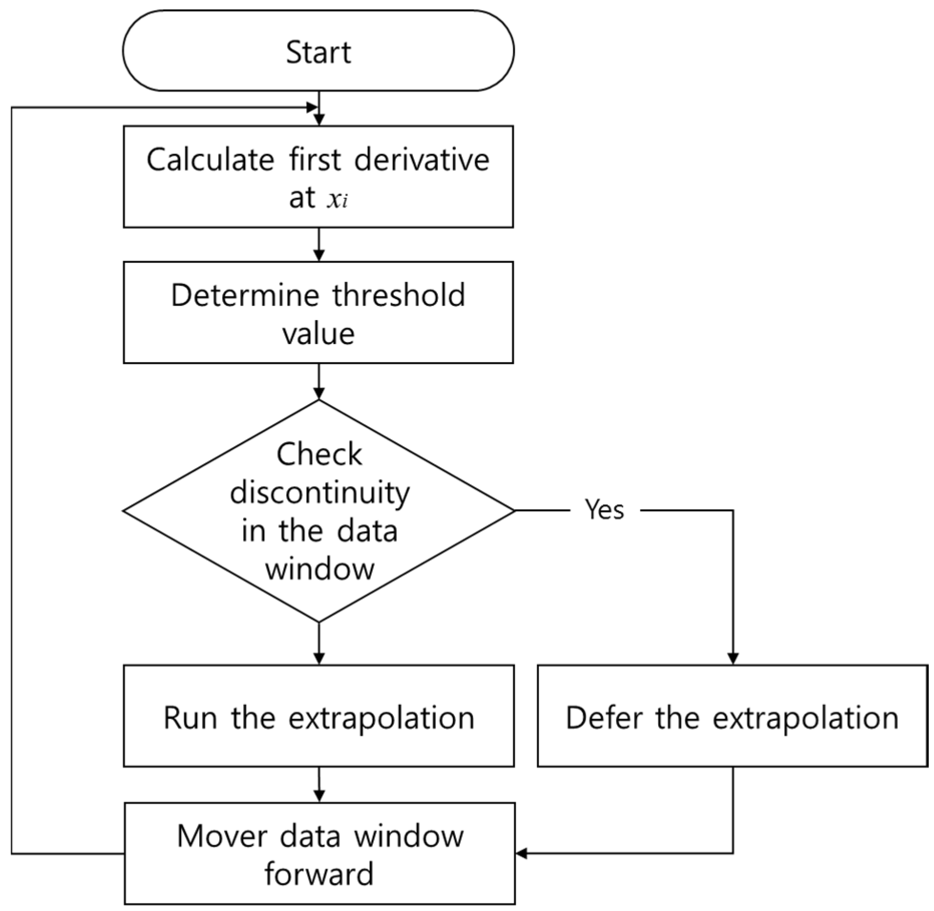
The first derivative of each xi, which is one of the equations for determining the spline polynomial coefficients, is compared with the heuristically determined threshold value to detect discontinuities. Discontinuity detection basically uses the slope of two successive data points thus magnitude, frequency and size of the computational time-step affect the threshold. kp is a heuristically determined constant which is generally in between 0.05 and 0.1 in 60 Hz system:
More frequent and periodic discontinuities, such as power electronic switching noise, are assumed to be eliminated or attenuated by harmonic filters; thus, a threshold is set to detect large disturbances such as transmission line faults which cause severe line voltage drop. Figure 7 shows that the spline extrapolation with discontinuity detection (spline/DD) effectively handles the numerical oscillation, which is unacceptably high in the normal spline method.
Figure 8 shows the interface node voltage between the capacitor and inductor of a simple R-L-C circuit [27], which demonstrates the time-step delay and the compensation effect on the co-simulation.
Both the dotted and dashed lines represent voltage waveforms, which are simulated with a 10 μs time-step, of the interface buses in each subsystem. The two voltage waveforms must be the same as the interface bus voltage waveform of the conventional simulation, which is represented by the solid line. However, phase and magnitude differences exist among the three voltage waveforms because the phase-shifted currents of subsystem 2, which result from the time-step delayed voltage signal generated by subsystem 1, are transferred back to subsystem 1 and input to the nodal equations. By using the proposed extrapolation method as Figure 9, the delayed voltage signal is successfully compensated and matches the reference signal.
3. Case Study
Two case studies which are an AC/DC system and an AC distribution system are used to verify the proposed framework. The cases are set up using PSCAD™. Each test system of the cases is divided into two subsystems. Each subsystem is run with two PSCAD programs concurrently which communicate each other via IPC.
3.1. AC/DC Power System
The AC/DC power system shown in Figure 10 is a simplified model of an island grid fed by a 300 MW HVDC system [28]. The selected information on the system is summarized in Table 1. A line commutated converter HVDC system continuously absorbs reactive power as part of the conversion process, and two synchronous condensers at the inverter bus supply reactive power to the HVDC system. The test system is partitioned into two subsystems along a fictitious bus at the inverter terminal. A frequency dependent network equivalent (FDNE) model based on vector fitting, which covers up to a 1 kHz frequency range, represents the AC equivalent circuit in the HVDC subsystem.
Figure 11 shows the comparison of three inverter bus AC voltage waveforms and their effect on the AC power injected by HVDC system. To show the delayed voltage signal effect on a simulation result more clearly the time-step is set to 100 μs.
As seen in Figure 11a a delayed voltage signal is well compensated by the proposed algorithm and reduces the error on the injected HVDC power to the AC system. The gap between the conventional simulation result and compensated co-simulation result is mainly due to the errors in the parameters in the FDNE model.
Figure 12 shows the grid frequency response to a bus fault. Each subsystem is simulated with a 10 μs time-step. At 0.1 s, a fault is applied to the inverter bus. The fault is successfully cleared after three cycles. Two real power values calculated at both sides of the interface bus deviate from the reference value from the conventional simulation because of the time delay, thus leading to inaccurate frequency response, as shown in Figure 12. The power deviation is successfully compensated for by the proposed extrapolation algorithm thus the results of the co-simulation match well with those of the conventional simulation.
3.2. AC Distribution System
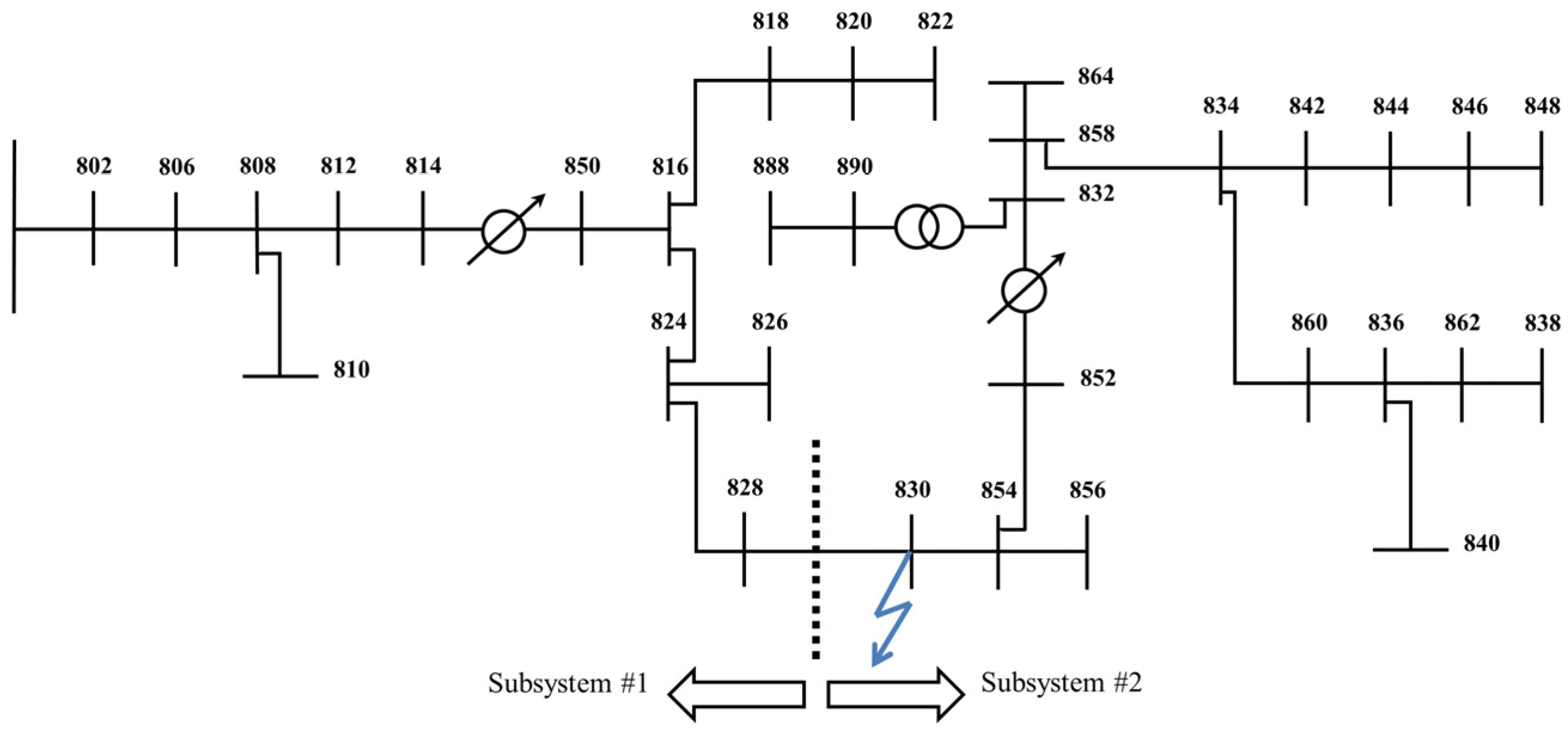
The AC distribution system is the IEEE 34 bus test feeder [29] (Figure 13). It is the complete data set of four radial distribution systems for analysis of unbalanced three-phase radial distribution feeders. It has been widely used as a test bench to evaluate the performance of newly developed technologies [30,31]. The selected information on the system specifications is summarized in Table 2.
It is divided into two subsystems at the sending end of the transmission line between the bus 828 and the 830 thus the subsystems have similar size and computational burden. The three phase ground fault is applied at the sending end of the transmission line between the bus 830 and the bus 854. The fault is applied at t = 0.2 s and cleared after three cycles.
As shown in Figure 14a the simulation result matches well to that of the conventional simulation which is shown in Figure 14b. Since two subsystems share one interface point the voltage and the current at the interface bus of each subsystem should be same as in Figure 15. The dashed line with square and the white circle which represent the interface bus voltage of the subsystem #1 and subsystem #2, respectively. The overshoot in the compensated signal appears to last longer than the reference signal due to the DD algorithm and the inaccuracy in the FDNE model parameters during the fault. However, after the overshoot the compensated signal quickly tracks the reference signal.
4. Conclusions
The speed of the conventional EMT simulation using both single-core and multi-core CPUs is similar because the conventional EMT simulation can hardly utilize the maximum computing power of a multi-core CPU. Co-simulation requires two concurrent simulations for the different subsystems, and inter-process communications between them. If the processor doesn’t handle this properly the two simulations will be executed in series, resulting in much longer computation time as is shown in Table 3. The proposed compensation algorithm effectively mitigates the negative impact of the time delay on co-operative EMT simulation thus enables to take advantage of the power of a multi-core CPU. It is a practical method as it can be applied to virtually all EMT simulation programs without source code modification.
Acknowledgments
This work (NRF-2015R1A2A2A01005497) was supported by Mid-career Researcher Program through NRF grant funded by the MEST and by the Power Generation & Electricity Delivery Core Technology Program of the Korea Institute of Energy Technology Evaluation and Planning (KETEP) granted financial resource from the Ministry of Trade, Industry & Energy, Republic of Korea (No. 20141010502280).
Author Contributions
Seaseung Oh contributed the simulation, analysis; Seaseung Oh and Suyong Chae wrote the paper.
Conflicts of Interest
The authors declare no conflict of interest.
Abbreviations
The following abbreviations are used in this manuscript:
| CPU | Central processing unit |
| DD | Discontinuity detection |
| EMT | Electromagnetic transient |
| FDNE | Frequency dependent network equivalent |
| GUI | Graphical user interface |
| HVDC | High voltage direct current transmission |
| IPC | Interprocess communication |
| R-L-C | Resistor, Inductor and Capacitor |
| SSE | Sum squared error |
References
- Chowdhury, S.P.; Chowdhury, S.; Crossley, P.A. UK scenario of islanded operation of active distribution networks with renewable distributed generators. Int. J. Electr. Power Energy Syst. 2011, 33, 1251–1255. [Google Scholar] [CrossRef]
- Dommel, H.W.; Meyer, W.S. Computation of electromagnetic transients. Proc. IEEE 1974, 62, 983–993. [Google Scholar] [CrossRef]
- Dommel, H.W. EMTP Theory Book; Bonneville Power Admin: Portland, OR, USA, 1986. [Google Scholar]
- Heffernan, M.D.; Turner, K.S.; Arrillaga, J.; Arnold, C.P. Computation of AC-DC System Disturbances—Part I. Interactive Coordination of Generator and Convertor Transient Models. IEEE Trans. Power Syst. 1981, 11, 4341–4348. [Google Scholar] [CrossRef]
- Gao, F.; Kai, S. Multi-scale simulation of multi-machine power systems. Int. J. Electr. Power Energy Syst. 2009, 31, 538–545. [Google Scholar] [CrossRef]
- Su, H.T.; Snider, L.A.; Chung, T.S.; Fang, D.Z. Recent advancements in electromagnetic and electromechanical hybrid simulation. In Proceedings of the International Conference on Power System Technology, Singapore, 21–24 November 2004; pp. 1479–1484.
- Lefebvre, S.; Mahseredjan, J. Interfacing Techniques for Transient Stability and Electromagnetic Transient Programs. IEEE Trans. Power Deliv. 2009, 24, 2385–2395. [Google Scholar]
- Hui, S.Y.R.; Fung, K.K.; Christopoulos, C. Decoupled simulation of DC-linked power electronic systems using transmission-line links. IEEE Trans. Power Electron. 1994, 9, 85–91. [Google Scholar] [CrossRef]
- Chiocchio, T.; Leonard, R.; Work, Y.; Fang, R.; Steurer, M.; Monti, A.; Khan, J.; Ordonez, J.; Sloderbeck, M.; Woodruff, S.L. A co-simulation approach for real-time transient analysis of electro-thermal system interactions on board of future all-electric ships. In Proceedings of the 2007 Summer Computer Simulation Conference, San Diego, CA, USA, 16 July 2007.
- Cécile, J.F.; Schoen, L.; Lapointe, V.; Abreu, A.; Bélanger, J. A Distributed Real-Time Framework for Dynamic Management of Heterogeneous Co-Simulations. Available online: http://www.rtlab.com/files/scs_article.pdf (accessed on 16 October 2015).
- Tylavsky, D.J.; Bose, A.; Alvarado, F.; Betancourt, R.; Clements, K.; Heydt, G.T.; Huang, G.; Ilic, M.; La Scala, M.; Pai, M.A. Parallel Processing in Power Systems Computation. IEEE Trans. Power Syst. 1992, 7, 629–638. [Google Scholar]
- Tomin, M.A.; De Rybel, T.; Marti, J.R. Extending the Multi-Area Thévenin Equivalents method for parallel solutions of bulk power systems. Int. J. Electr. Power Energy Syst. 2013, 44, 192–201. [Google Scholar] [CrossRef]
- Su, H.T.; Chan, K.W.; Snider, L.A. Parallel interaction protocol for electromagnetic and electromechanical hybrid simulation. IEEE Proc. Gener. Trans. Distrib. 2005, 152, 406–414. [Google Scholar] [CrossRef]
- Marti, J.R.; Linares, L.R.; Calvino, J.; Dommel, H.W.; Lin, J. OVNI: An object approach to real-time power system simulators. In Proceedings of the International Conference on Power System Technology, Beijing, China, 18–21 August 1998; pp. 977–981.
- Sultan, M.; Reeve, J.; Adapa, R. Combined transient and dynamic analysis of HVDC and FACTS systems. IEEE Trans. Power Deliv. 1998, 13, 1271–1277. [Google Scholar] [CrossRef]
- Wang, Y.P.; Watson, N.R. A benchmark test system for testing frequency dependent network equivalents for electromagnetic simulations. Int. J. Electr. Power Energy Syst. 2013, 44, 364–374. [Google Scholar] [CrossRef]
- Annakkage, U.D.; Nair, N.-K.C.; Gole, A.M.; Dinavahi, V.; Noda, T.; Hassan, G.; Monti, A. Dynamic system equivalents: A survey of available techniques. IEEE Trans. Power Deliv. 2009, 27, 411–420. [Google Scholar] [CrossRef]
- Gustavsen, B.; Semlyen, A. Rational approximation of frequency domain responses by vector fitting. IEEE Trans. Power Deliv. 1999, 14, 1052–1061. [Google Scholar] [CrossRef]
- Gustavsen, B.; Mo, O. Interfacing convolution based linear models to an electromagnetic transients program. Int. Conf. Power Syst. Trans. 2007, 1, 4–7. [Google Scholar]
- Zhu, W.; Pekarek, S.; Jatskevich, J.; Wasynczuk, O.; Delisle, D. A Model-in-the-Loop Interface to Emulate Source Dynamics in a Zonal DC Distribution System. IEEE Trans. Power Electron. 2005, 20, 438–445. [Google Scholar] [CrossRef]
- Wu, X.; Lentijo, S.; Deshmuk, A.; Monti, A.; Ponci, F. Design and implementation of a power-hardware-in-the-loop interface: A nonlinear load case study. In Proceedings of IEEE Applied Power Electronics Conference and Exposition, Austin, TX, USA, 6–10 March 2005; Volume 2, pp. 1332–1338.
- Ren, W.; Steurer, M.; Woodruff, S.; Andrus, M. Demonstrating the Power Hardware-in-the-Loop through Simulation of a Notional Destroyer-Class AllElectric Ship System during Crashback. In Proceedings of the ASNE Advanced Propulsion Symposium, Arlington, VA, USA, 30 October 2006.
- Noda, T.; Sasaki, S. Algorithms for distributed computation of electromagnetic transients toward pc cluster based real-time simulations. In Proceedings of the International Conference on Power System Transients, New Orleans, LA, USA, 28 September 2003.
- Dufour, C.; Paquin, J.-N.; Lapointe, V.; Be’langer, J.; Schoen, L. PC cluster-based real-time simulation of an 8-synchronous machine network with HVDC link using RT-LAB and TestDrive. In Proceedings of the 7th International Conference on Power Systems Transients, Lyon, France, 4–7 June 2007.
- Ren, W.; Steurer, M.; Woodruff, S. Accuracy evaluation in power hardware-in-the-loop (PHIL) simulation center for advanced power systems. In Proceedings of the 2007 Summer Computer Simulation Conference, San Diego, CA, USA, 16 July 2007.
- Fang, T.; Chengyan, Y.; Zhongxi, W.; Xiaoxin, Z. Realization of electromechanical transient and electromagnetic transient real time hybrid simulation in power system. In Proceedings of the IEEE/PES Transmission and Distribution Conference Exhibition, Dalian, China, 14 August 2005; pp. 1–6.
- Belanger, J.; Snider, L.A.; Paquien, J.; Pirolli, C.; Li, W. A Modern and Open Real-Time Digital Simulator of Contemporary Power Systems. In Proceedings of the International Conference on Power Systems Transients (IPST 2009), Kyoto, Japan, 2 June 2009; pp. 2–6.
- Jang, G.; Oh, S.; Hann, B.-M.; Kim, C.K. Novel reactive power compensation scheme for the Jeju-Haenam HVDC system. IEEE Proc. Gener. Trans. Distrib. 2005, 152, 514–520. [Google Scholar] [CrossRef]
- Kersting, W.H. Radial distribution test feeders. In Proceedings of the 2001 Power Engineering Society Winter Meeting, Columbus, OH, USA, 31 January 2001; Volume 2, pp. 908–912.
- Jang, S.; Kim, K. An islanding detection method for distributed generations using voltage unbalance and total harmonic distortion of current. IEEE Trans. Power Deliv. 2004, 19, 745–752. [Google Scholar] [CrossRef]
- Xin, H.; Qu, Z.; John, S.; Ali, M. A Self-Organizing Strategy for Power Flow Control of Photovoltaic Generators in a Distribution Network. IEEE Trans. Power Deliv. 2011, 26, 1462–1473. [Google Scholar] [CrossRef]
Figure 1.
Network partitioning.

Figure 2.
Parallel interface protocol.

Figure 3.
Inter-process communication (IPC) process of co-simulation.

Figure 4.
Prediction error comparison for a chirp signal.

Figure 5.
Iterative extrapolation of a two step forward estimation.

Figure 6.
Summation of squared error (SSE) variation in the spline extrapolation.

Figure 7.
Discontinuity detection effect on the numerical oscillation.

Figure 8.
Interface node voltage during resistor, inductor and capacitor (R-L-C) energization.

Figure 9.
Extrapolation process of the discontinuity detection (DD) algorithm.

Figure 10.
AC/DC test system.

Figure 11.
The effect of the compensation on (a) the voltage and (b) the high voltage direct current (HVDC) power.
Figure 11.
The effect of the compensation on (a) the voltage and (b) the high voltage direct current (HVDC) power.

Figure 12.
AC grid frequency during a bus fault at the inverter bus.

Figure 13.
IEEE 34 bus test system.

Figure 14.
Three-phase ground fault simulation using (a) proposed framework and (b) conventional simulation.
Figure 14.
Three-phase ground fault simulation using (a) proposed framework and (b) conventional simulation.

Figure 15.
Zoomed view of the phase A voltage comparison at the fault.


| Specifications | HVDC System | AC System |
|---|---|---|
| Type | Line commutated converter | |
| Rate Voltage | DC ±180 kV | 154 kV |
| Rate Current | 849 A | - |
| Rating | 300 MW | 75 MVA synchronous generator |
| Number of circuits | 2 | - |
| Converter Transformer | 3phase 3winding (YDY) | - |
| Reactive power compensation | 70 MVA synchronous condensers | - |
| Harmonic Filter | DTF 27.5 MVA X 2 for 11, 13th harmonics HPF 27.5 MVA X 2 for 23, 25th harmonics | - |
| Type | Radial |
|---|---|
| Total Number of Bus | 34 |
| Frequency | 60 Hz |
| Voltage | 24.9 kV |
| Number of Loads | Spot: 6, Distributed: 19 |
| Total Load | Active: 1769 kW, Reactive: 1044 kW |
| Transformer | 24.9 kV/4.16 kV, D-Y, 500 kVA |
| Voltage Regulator | Y-Y with OLTC |
| Shunt Capacitor | 750 kVA |
| Type | Conventional | Co-simulation | ||
|---|---|---|---|---|
| Case | Reference | Common time-step | ||
| CPU | Single core (3.2 GHz) | Multi core (2.66 GHz) | Single core (3.2 GHz) | Multi core (2.66 GHz) |
| Time-step | 10 μs | 10 μs | 10 μs | 10 μs |
| Computation time * | 1 | 1.12 | 6.72 | 0.51 |
* normalized by the reference case.
© 2016 by the authors; licensee MDPI, Basel, Switzerland. This article is an open access article distributed under the terms and conditions of the Creative Commons by Attribution (CC-BY) license (http://creativecommons.org/licenses/by/4.0/).
Share and Cite
MDPI and ACS Style
Oh, S.; Chae, S. A Co-Simulation Framework for Power System Analysis. Energies 2016, 9, 131. https://doi.org/10.3390/en9030131
AMA Style
Oh S, Chae S. A Co-Simulation Framework for Power System Analysis. Energies. 2016; 9(3):131. https://doi.org/10.3390/en9030131
Chicago/Turabian StyleOh, Seaseung, and Suyong Chae. 2016. "A Co-Simulation Framework for Power System Analysis" Energies 9, no. 3: 131. https://doi.org/10.3390/en9030131
Note that from the first issue of 2016, this journal uses article numbers instead of page numbers. See further details here.