1. Introduction
Korea is the fifth largest oil importer in the world. Since Korea does not produce oil, 97% of the fossil fuel used for energy is imported [
1]. As a result, saving energy has increasingly become an important part of national policy. As buildings account for around 30% of energy consumption, energy efficiency should be improved and more renewable energy sources used to prepare for rising energy costs and evolving international environmental regulations. Energy policy for buildings includes strengthening the energy saving standards of a building, such as the U-value of the building envelope, or enforcing compulsory use of renewable energy sources. To adjust to these measures, however, construction companies have been meeting only the minimum standard each time regulations are tightened. This is caused largely by the misunderstanding that efforts to reduce energy consumption undermine profitability, meaning that energy saving buildings are not attractive to investors who wish to maximize profit.
According to prior research [
2], a lack of information on the return period of an energy reduction investment or an energy saving strategy is a stumbling block for people to invest in energy saving processes. The cost of collecting the energy data or installing new energy-efficient equipment is hard to recognize as a cost saving investment when compared with the simple purchase of energy. This can be a greater obstacle to small and medium-sized enterprises. To overcome this, financial information such as life cycle cost should be gathered for the decision-making process of the building design. Architects experience many difficulties in the process of designing buildings with reduced energy consumption, one way of which is to find an optimal combination of the many variables that affect energy savings. As they cannot analyze all possible design alternatives and complex situations in the design process, it is difficult for them to be certain that this is the optimal design, despite undertaking numerous energy simulations. A model that can find the optimal combination using an algorithm would help to arrive at the optimal energy saving design in a timely manner. It is hard to decide if a building is a good investment in terms of the life cycle cost, even if an optimal building design that uses the least energy is produced. If a cost optimization model can be suggested, with application of all energy saving elements in the design process and the life cycle cost taken into consideration, companies may actively participate in constructing buildings that use less energy. In this context, this study aims to suggest a model that minimizes the life cycle cost through combined use of interactive energy saving strategies. It also presents the need for, and applicability of, the cost optimization model by applying this model to an industrial building with high energy consumption, a topic not yet addressed in previous studies.
2. Research and Development of Mobile Applications for Building Construction
2.1. Type and Characteristics of Optimization Technique
Optimization is the process of finding the best outcome amongst available alternatives that meet given requirements under given circumstances. It is also a method for isolating the global optimum within a given design space. The basic items required to perform an optimization are the design variables, objective functions and constraints. The following expresses optimization in a general mathematical sense.
Here,
X represents design variables consisting of design vectors, and
f(
X) is a design vector consisting of the objective function. The constraints of the design vector is g
i (
X) ≤ 0,
i = 1, 2, …,
m and
lj (
X) = 0,
j = 1, 2, …,
p [
3]. Determining the design variables, objective functions and constraints is the most important part of the procedure and requires the optimization technique. There are various optimization techniques which are used, depending on the constraints, the number of objective functions and many other classification criteria. These methods are generally classified as either deterministic or stochastic.
A deterministic method seeks a local minimum and uses a convex function, mostly based on the gradient method. Simplex methods and pattern search methods, however, are deterministic methods that do not take the form of a convex function. When a function has an exact solution, the calculations are fast. However, these methods are difficult to apply to non-linear problems and problems that cannot be solved with differentiation. In some cases, local minima, which are attained in a manner dependent upon the start point, are recognized as the optimal minima. Stochastic methods find a global optima based on a random search procedure. This is therefore a non-gradient method and uses only the function value for comparison. This category includes Simulated Annealing [
4], Evolution Strategies [
5], Genetic Algorithms [
6], Tabu Search methods [
7] and Differential Evolution [
8]. These methods are effective at finding the global minima in non-linear problems and problems that cannot be solved with a differential, but can take much longer when compared with gradient methods.
2.2. Building Energy and Cost Optimization Resear
Recent building energy optimization studies at home and abroad have applied optimization from the design to the large-scale system. Interest in optimal control during operation has also increased beyond the design stage. This is in contrast to empirical analysis which uses energy savings as the sole parameter of the energy analysis program during design. Multi-objective optimizations have been applied with multiple optimization targets (objective functions) through use of the genetic algorithm [
6], the Taguchi-ANOVA method [
9] and the PSO algorithm [
10] as optimization techniques.
Recent studies on cost optimized industrial buildings published in other countries [
11,
12,
13,
14,
15] estimated all costs, including the building energy, reduction of CO
2 emissions and life cycle cost. However, Korean studies [
16,
17,
18,
19] have limited their scope to the optimal construction costs, focusing on structure, materials and construction. Since many studies on optimizing the life cycle cost have considered energy, they applied the optimization technique by recognizing the outcome of the building energy analysis program as a cost. Therefore, the optimization technique also used a genetic algorithm (GA), an evolutionary algorithm and Tchebycheff optimization, similar to those used for energy optimization.
2.3. Building Energy and Cost Optimization and Genetic Algorithm (GA)
Optimization of the building energy and cost results in a multi-dimensional solution space must use a multi-objective optimization method, with the solution space having several local minima. The solution space is also characterized by discontinuities and non-linearity, with discrete and continuous variables existing together [
20,
21,
22]. As a result of the size of the solution space, it is impossible to check all possible combinations. Seeking a solution using a gradient method is also impossible as many objective functions cannot be differentiated [
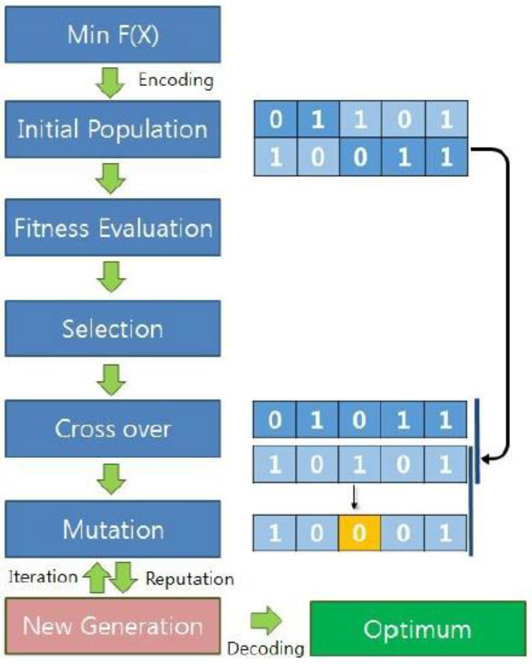
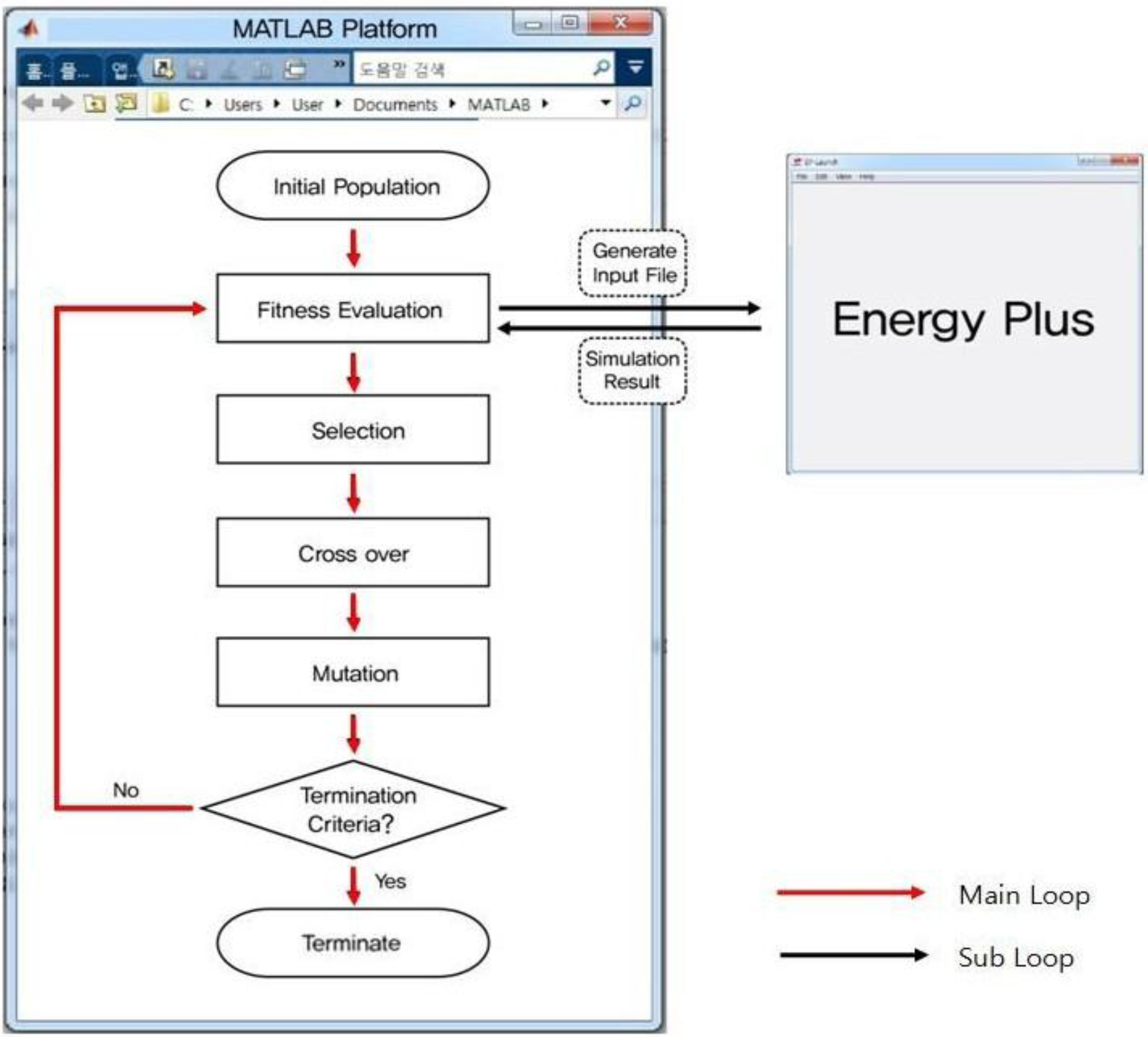
23]. To find the correct method for such an optimization problem, this study reviewed the aforementioned optimization techniques. As a result, it is believed that, though the calculation is slower than with the gradient method, a non-gradient, stochastic method that is appropriate for non-linear and non-differentiable problems would be the best to locate the global minima. A genetic algorithm (GA), selected good designs by including combinations of variables to form the chromosomes, then evaluating the appropriateness and forming the next generation using an algorithm that ultimately produces the optimal solution (
Figure 1).
3. Life Cycle Cost (LCC) Analysis and Optimization Method
3.1. Need for LCC Analysis
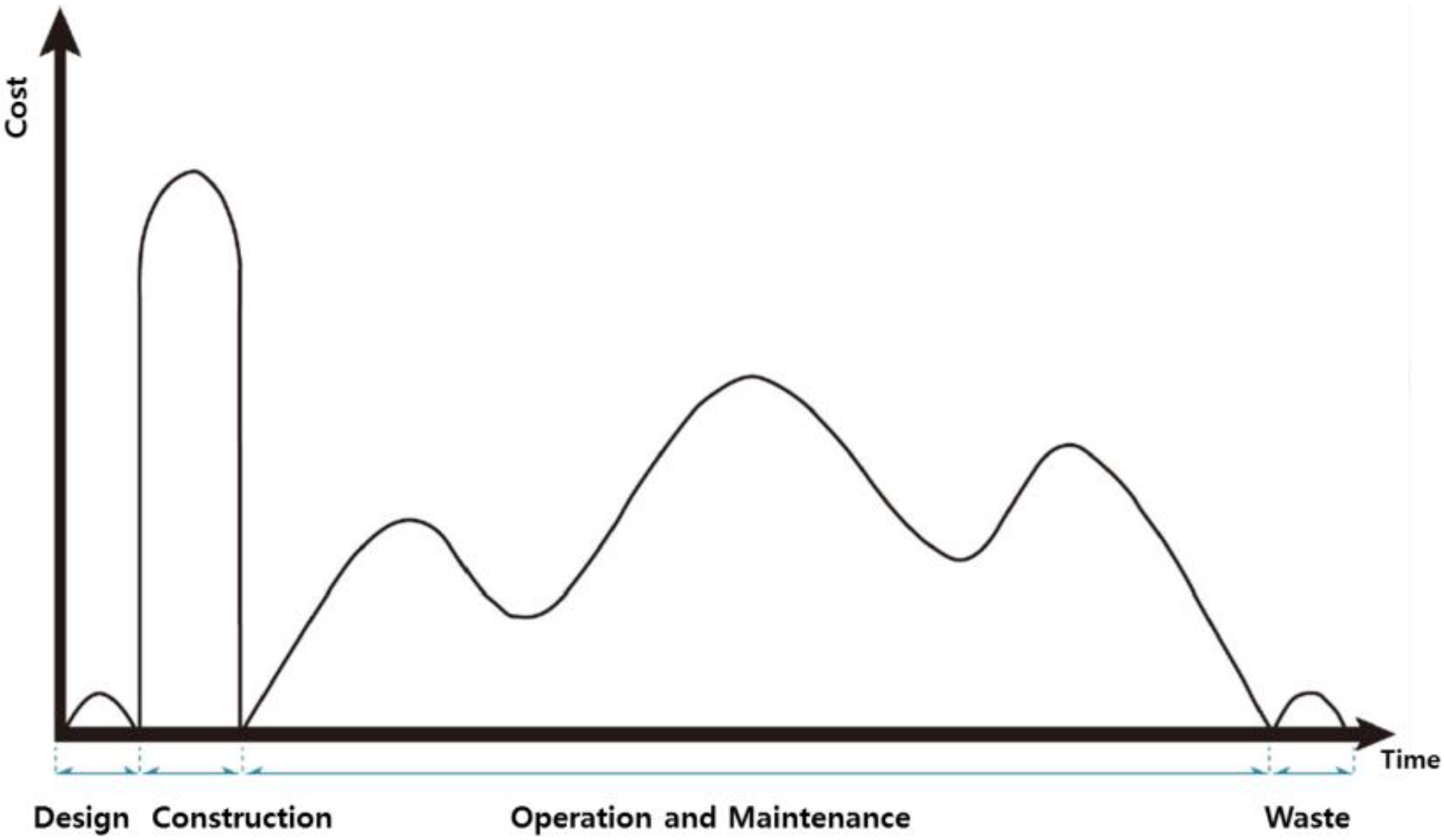
Generally, buildings have a life cycle formed of planning, design, construction, maintenance, demolition and removal, with maintenance also accounting for a high proportion of the total cost. LCC data from the US and Japan [
24,
25] show that maintenance requires about three-to-five times the initial investment, as seen in
Figure 2. Since the planning, design and construction stages are classified as the initial investment cost, usually excluding short-term operations costs, investment is not straightforward without a long-term vision.
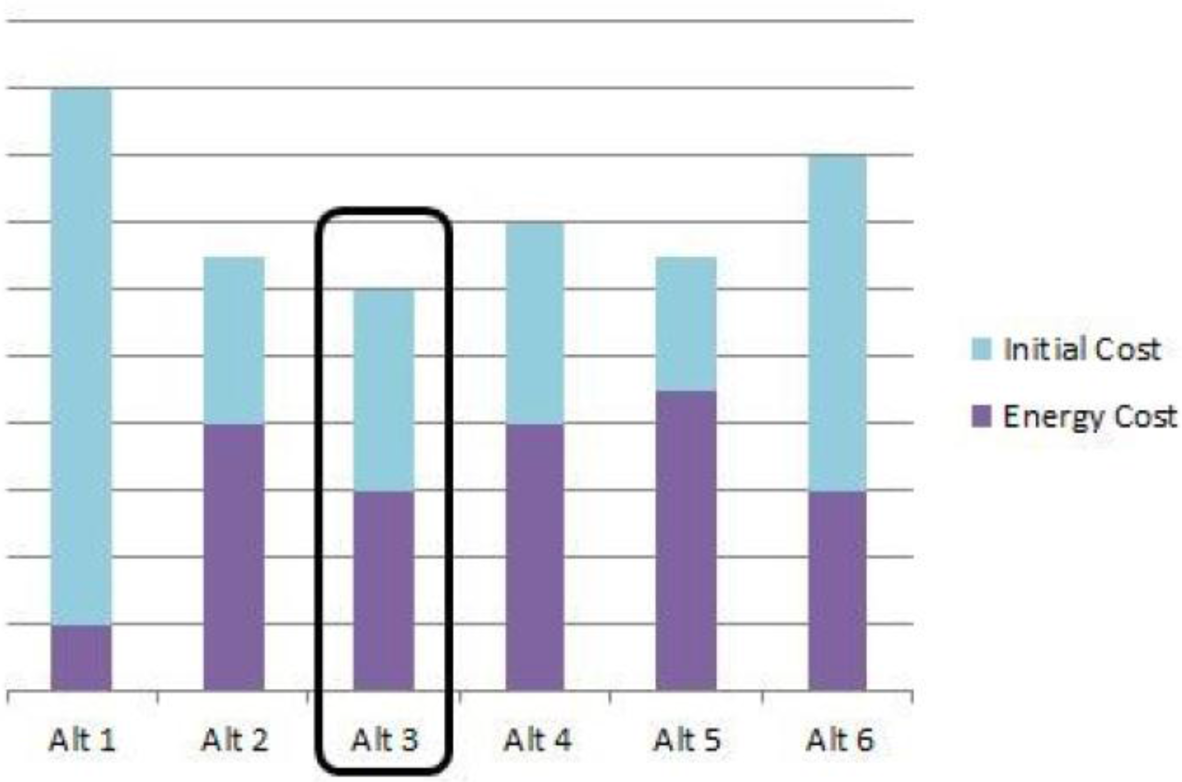
If the operational or environmental costs (CO
2 emission costs) needed for building maintenance were predicted and provided as cost data, a high initial investment can be recognized as being reasonable from the perspective of the total expense. Interest in the environment and reducing energy consumption are increasing, and the national certificate system and energy saving laws evolve accordingly. As the energy saving methods are interactive, their effects may sometimes clash with one another. As a substantial initial investment does not bring about a proportionate reduction of the energy cost, the total cost of designing energy saving buildings needs to be analyzed. For instance, in
Figure 3, Alternative 1 would be selected if only energy savings were considered. However, if the total cost were to be analyzed, Alternative 3 would be chosen. Therefore, prediction and analysis of the LCC in the initial design stage is increasingly emphasized to assist in making wise investment decisions as energy use reduction becomes obligatory for buildings.
3.2. Assumption and Condition for LCC Analysis
As a building life cycle occurs over the long term, setting up important variables in the LCC analysis is vital. An accurate and reasonable analysis requires a realistic setup. However, an LCC analysis is a prediction, and estimation of future costs is uncertain and depends upon the underlying assumptions. Therefore, factors to be designated as LCC analysis variables should be determined based upon the most objective grounds. LCC analysis factors include the analysis period, discount rate and inflation. This study used a real discount rate that is also used to convert utilization into an actual time value, considering the opportunity cost at the same time. In the process of estimating the LCC, costs that occurred throughout the period in question should be calculated at a certain point in time. This study used the present value method to calculate the value of all future costs at the current value.
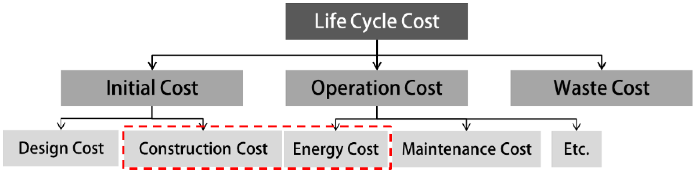
Cost items to be applied in an LCC analysis should be set up depending on the analysis objective, where either the entire building or a certain objective in the building can be considered. An LCC analysis can affect decision making. This study classified the items that formed a substantial cost as the major cost items to help make the correct investment decisions and made them the analysis target. Similar fixed costs present in all alternatives were not classified as variables in the selection process. The most influential cost items reflecting the energy saving strategies in the building design were the materials component of the initial investment along with the installation costs and the energy costs during operation. Therefore, this study estimated the cost of the two stages of the life cycle to analyze the LCC (
Figure 4).
3.3. Optimization Modeling of LCC Analysis
The initial investment in LCC components can be described with a relatively simple functional formula when there is cost data per unit area. However, the operating cost cannot be described so simply as it is affected by external conditions such as the weather, season and solar altitude. To address this problem, the optimization technique used MATLAB (main loop) and wrote a double loop so that only the energy cost of the building could be drawn through the building energy simulation performed in Energy Plus (sub-loop). Energy Plus received the newly produced IDF file from MATLAB (Energy Plus file format) as an input and sent the simulation results to MATLAB as an output (
Figure 5) [
19].
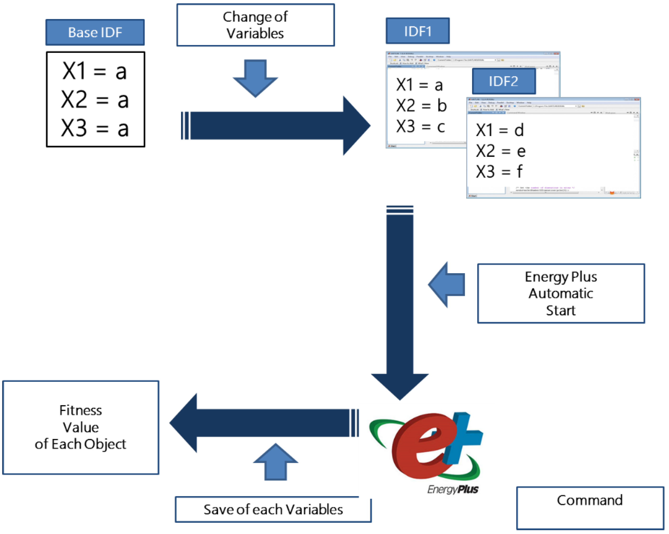
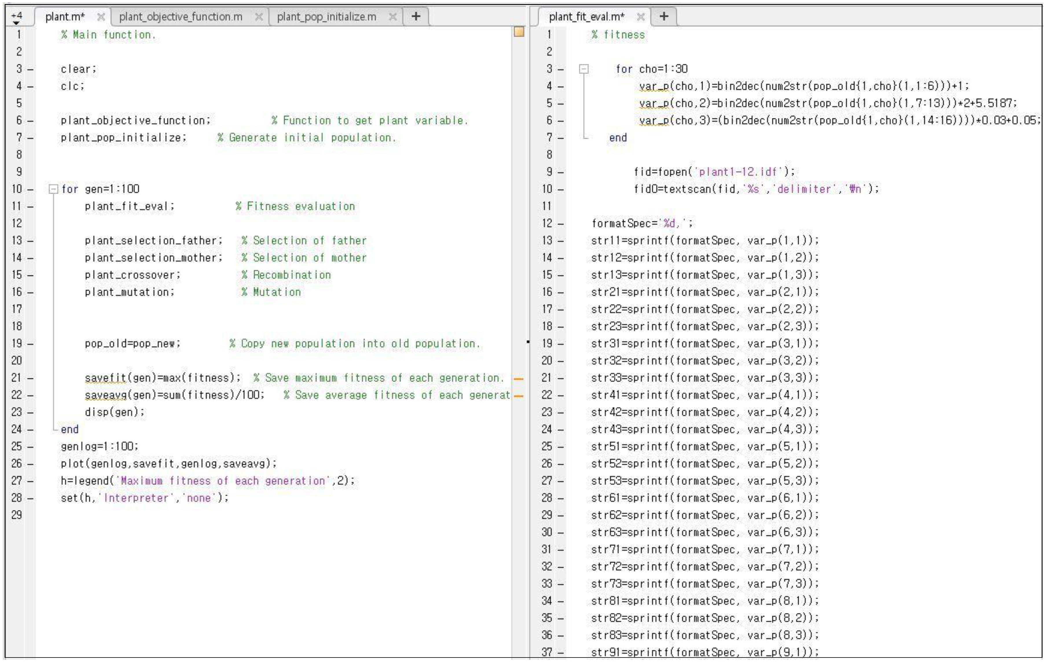
When individuals of the early generations were arbitrarily created through the GA implemented in MATLAB, new IDF files were created, with each individual contained in the basic IDF file (Energy Plus file format). Since one IDF file has one combination of design variables, the building energy consumption was estimated as the design variable inside each IDF file when Energy Plus was automatically set to run. This value was then read in MATLAB and used to write a fitness function. If this process were manual, it would be time consuming and so an M file script (M-Script) was created to run automatically inside the MATLAB platform (
Figure 6). The results from the fitness evaluation were input to the GA, which found the optimal solution by repeating for the maximum allowable number of generations.
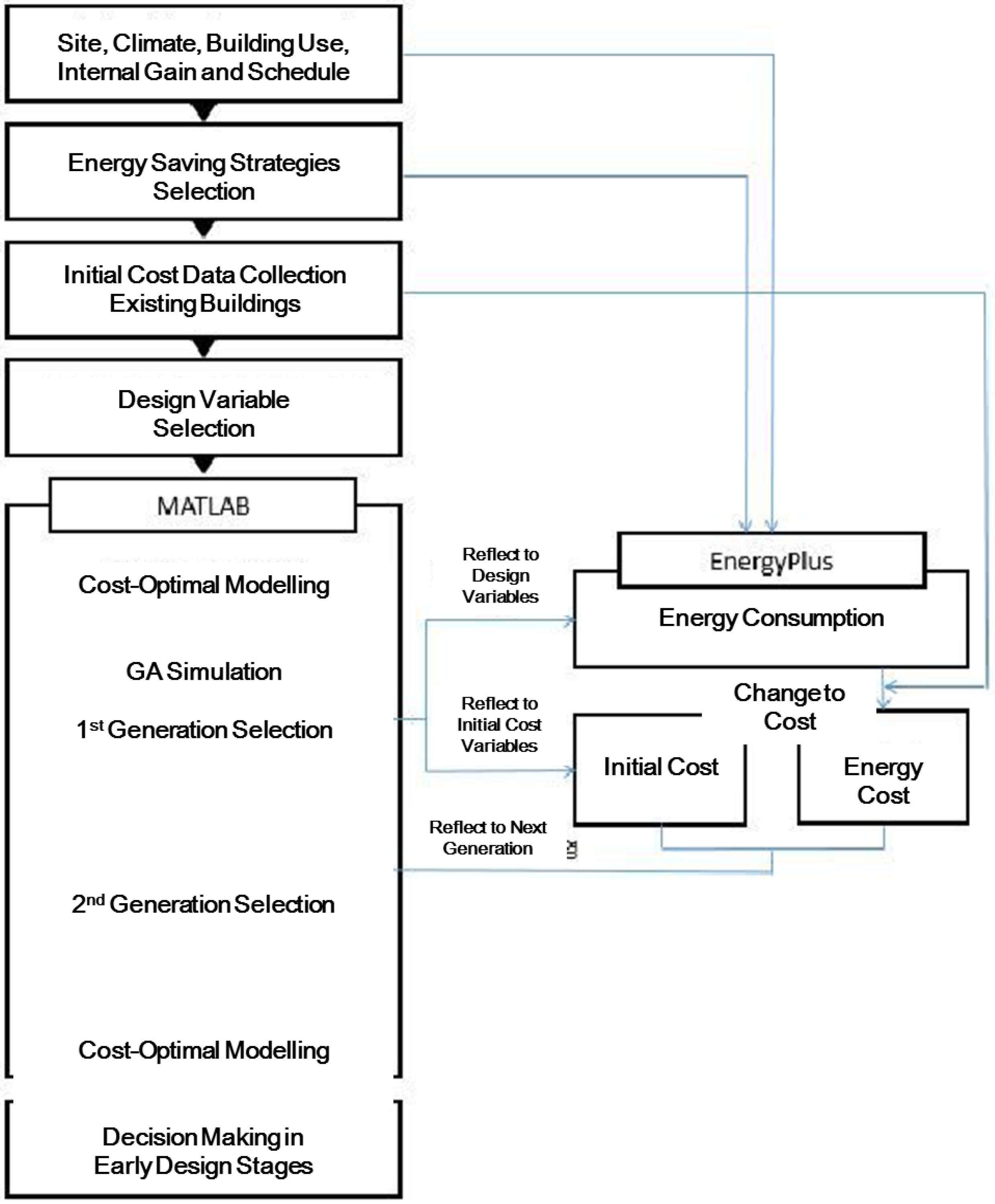
The following
Figure 7 showed the process of drawing the cost optimization model considering energy saving.
4. Energy Simulation on the Target Building
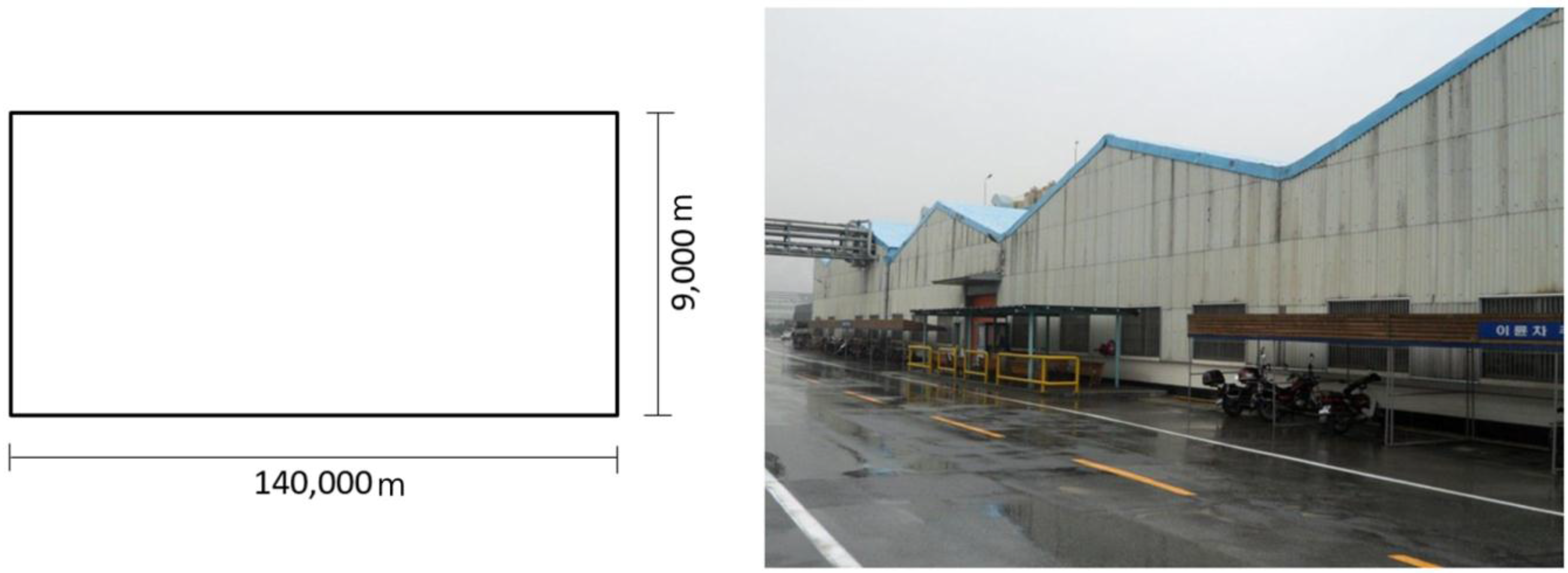
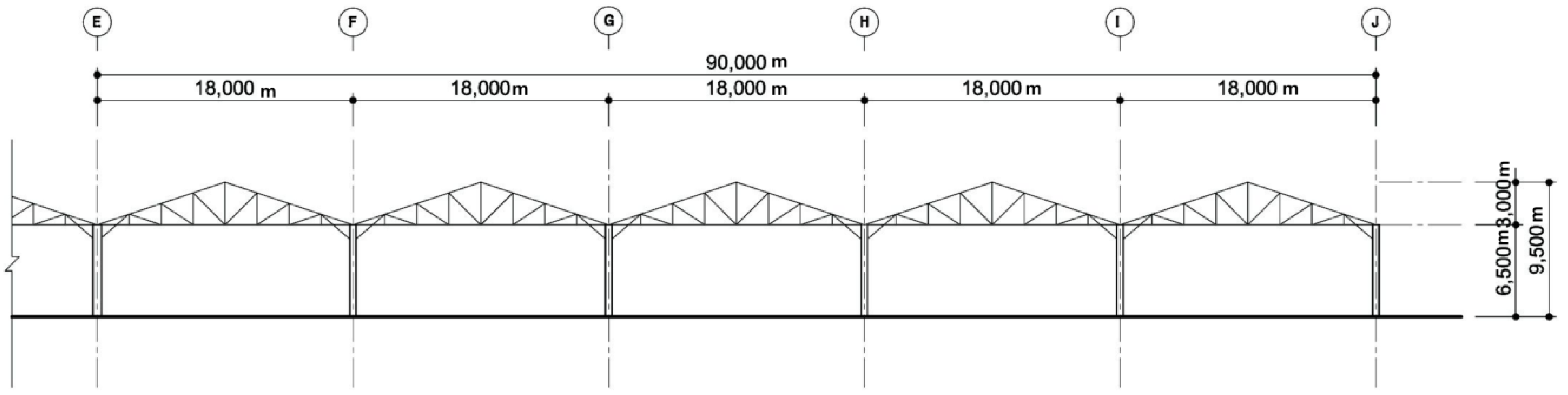
This study selected a building and performed a case study to illustrate the cost optimization model’s use in the energy saving design. As previous studies on building energy and optimal costs were focused on residential and office buildings instead of industrial ones, an industrial building was purposely selected. The chosen building is an automobile factory in Ulsan, Korea, with one-quarter of it being examined in the study. With a gross floor area of 12,600 m
2 (140 m × 90 m) and a height of 6.5 to 9 m, it is a single-story, open space building. The building has an 18 m gable roof, with five rooftops (
Figure 8).
4.1. Characteristics of Industrial Buildings
Unlike other buildings, industrial buildings need a large-scale space plan, considering the large manufacturing equipment and products which they must accommodate. These buildings have a multitude of large open spaces to carry out work and a wide envelope compared with the area used. Above all, the roof area takes up a great proportion. The roof type is an important parameter in this building type as it has a close relationship with the building’s manufacturing features, natural lighting and ventilation. The roof types of industrial buildings are closely related with the manufacturing process employed. Types include flat roofs, gable roofs, monitor roofs, saw-tooth roofs,
etc., and they are built depending on the manufacturing characteristics, with consideration of the pillar intervals, ventilation and natural lighting plan [
26]. To prevent leaks at the joints, the roof slope was steep in the 1970s (3/10 gradient) and heat insulation materials were not used. In the 1980s, the slope became less steep (1/10) and insulation materials began to be applied. From the 1990s, roofs could be constructed to be seamless, making the slope even easier (3/100). A body shop (the subject of this study) of an automotive factory is the place where robots weld the panels from the press factory to produce automobile frames. Bogies move the frames and inspection robots are in place for quality control. It is therefore important to consider the inside flow and the movement of logistics entering from outside [
27]. The side windows of the building envelope are not enough to light deep inside an automotive factory, which has a wide internal space; therefore, natural light coming through skylights in the roof is more effective. There are, additionally, skylights and clerestory and topside lighting systems which are employed. The machines used are heavy and their vibrations sometimes violent, meaning that the body shop is usually built as a single-story building. As the most common structure of an industrial building, it provides good conditions for horizontal transportation of materials and equipment. Since a single-story building is high, natural lighting and illumination are provided through skylights for the working area. Because of its height, however, ascending air currents cause excessive thermal stratification and the large envelope area also brings about great heat loss and heat gain. Because of the large machines, equipment and the continuous logistics flow, a gable roof that offers wide pillar intervals is preferred.
4.2. Energy Saving Strategies in Industrial Buildings
It is assumed that manufacturing equipment uses 30% of the total energy consumption, with cooling/heating and lighting accounting for 40% and 30%, respectively. Though it may vary depending on manufacturing processes, the lighting load can account for up to 40% of total energy use [
28]. Energy consumption caused by the manufacturing equipment inside of the industrial building is not directly affected by the building design. However, the remaining energy use can be saved through the design. As previously mentioned, the building has a wide surface area to account for the equipment size, work flow and movement, with the roof accounting for around 70% of the total surface area [
29]. As the roof angle has been reduced thanks to advanced construction technology, the roof received more solar heating than it could have with vertical elements. As the roof plays a significant role in transmitting solar radiation energy indoors, substantial effects were expected if energy saving items were applied to the roof.
The energy saving items the study selected were:
Photovoltaic (PV) panels: The roof has many advantages for the use of PV systems. PV panels on the roof will not experience reduced efficiency from shadows, and the sloped roof is ideal to receive sunlight. They are often used on the sloped roof to the south and are expected to produce a high power generation efficiency after installation [
30]. PV panels installed on the roof whose minimum pitch is 3/10 to the south, will convert solar radiation with an efficiency of around 90% [
31].
Natural lighting through a skylight: This is appropriate for an industrial building that has a single-story open space with great height. Because lighting with direct sunlight is difficult in an area that frequently has a clear sky, it is necessary to block the light with a sunshade or to convert it to diffused light. There are also benefits to inviting the sunlight from the north using a saw-tooth roof [
32].
Improved roof insulation: The envelope of the roof accounts for more than 70% of the total envelope. Such roofs were constructed mainly with asbestos cement slate in the 1970s and 1980s and sandwich panels followed. The sandwich panels are made up of steel plates with insulation materials in between. The insulation materials between the steel plates have a significant influence on the thermal transmittance of the entire envelope [
33].
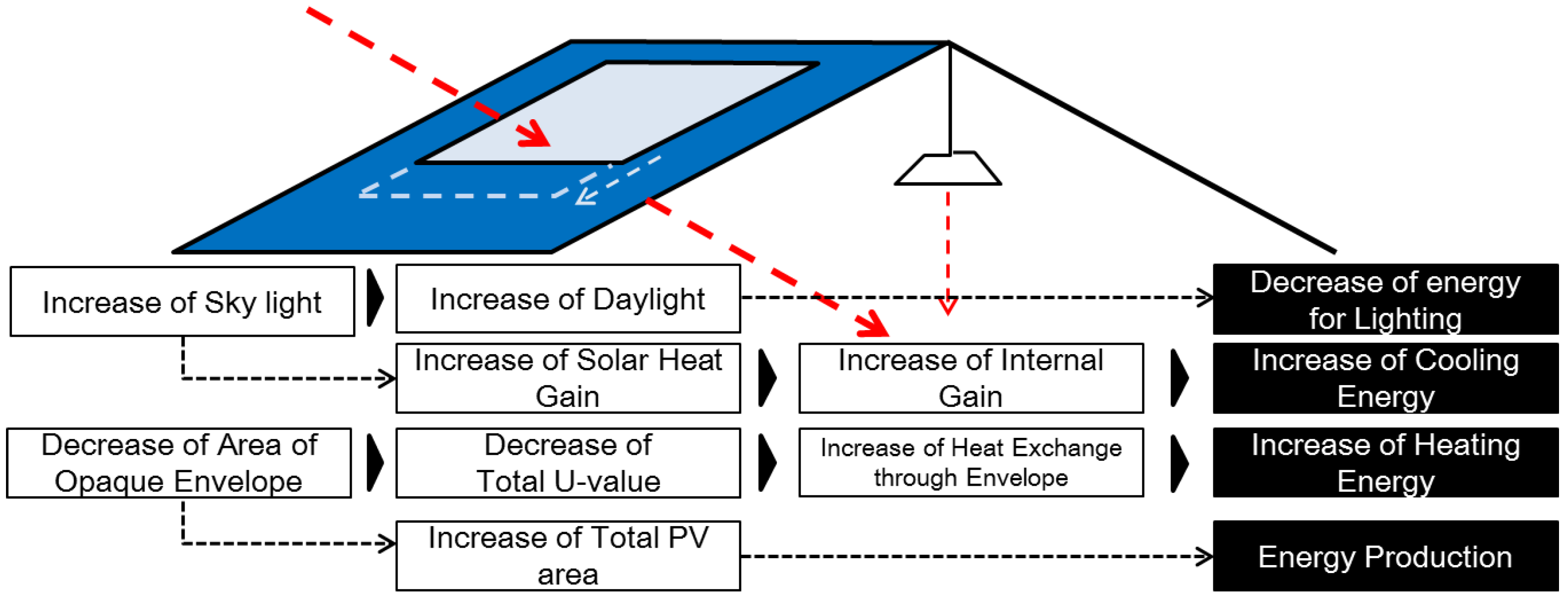
Each of these energy saving items were proven effective at saving energy by many studies. They also create synergy through their interaction, though conflicting effects have been noted as well (
Figure 8). To find the optimal combination of items, this study applied the method seen in
Figure 9.
4.3. Energy Simulation
The basic information for the energy analysis is detailed below in
Table 1. The energy simulation was conducted in Energy Plus and, unlike other software, it uses its own IDF file format which is compatible with other programs so as to be text-based and re-writable. As it is compatible with the optimization program for the optimization model, it was selected as the energy analysis instrument.
This study used the internal gains from a previous study [
34] on the same industrial building, but revised them to accommodate the reduced model size. Robots account for most of the machines inside the industrial building and each process (No.1 and No.2) has 45 robots. The power consumed by one robot is 1527 W, meaning that 90 robots use 137,430 W. The thermal density per unit area was estimated at 14.0 W/m
2. The industrial building which houses Process 1 and 2 has a total of 84 workers, with 42 on each process. ASHRAE Fundamental [
35] was used as a reference for the working conditions and heat generation from the occupants. Considering the type of work in the building, this study used a heat value of 110 W and a latent heat of 185 W for light machine work. The building uses four fluorescent lamps (40 W) hanging from each skylight and has a lighting density of 4.4 W/m
2. The building operates Monday through Friday and the daily working hours are eight hours on the day shift and eight at night, making 16 h in total. This study used the Air Flow Network model of Energy Plus to apply an annual infiltration (0.31~0.6ACH) and used a value of 3.28ACH, which added the ventilation rate of the exhaust fans to the simulation based on the supply airflow and exhaust fan of each process.
Table 2 below showed the performance of the PV modules installed on the five roof surfaces facing south.
The five roof surfaces facing north were installed with skylights, with the illumination required for light work set at 300 lux to make the most of the natural light. The working surface was 0.85 m above the ground and illumination sensors were installed at two locations inside the building.
5. Establishment of Cost Optimal Industrial Building Model
5.1. Setup for LCC Analysis on the Industrial Building
From the national tax regulation [
36], a 20-year analysis period was decided, assuming that the standard durable years of the steel/concrete factory is 20 years. A real discount rate was applied using Equation (1). As it is very difficult to predict both the interest rate and inflation, since they change every year, an arithmetic mean of the real discount rate calculated from data from the last 10 years (2005 to 2014) was applied. The arithmetic mean of the data for the last decade resulted in a figure of 1.32%. The interest rate used for the calculation came from the time deposit data (five years or more) of the Bank of Korea economic statistics system [
37], while the consumer price index and inflation data came from the Korean Statistical Information Service [
38].
The initial investment only considered the parts to which the energy saving items were applied. PV panels are subject to support provided by the Ministry of Trade, Industry and Energy according to its renewable energy policy (building support program). The national regulations include financial support and around 26% of the cost was subsidized in 2015. This referred to a glass estimate from Hankuk Glass Industries and the Korea Price Research Center (Seoul, Korea) and estimated the unit roof price with actual construction cases from S Architect and Engineers. The operating electricity cost used the industrial power I, voltage A and selection I, provided by Cyber Korea Electric Power Corporation (KEPCO) (Seoul, Korea), so that the data can be converted into a unit price per kW.
Table 3 shows the power cost data from 21 November 2013.
5.2. Setup for Cost Optimal Building
5.2.1. Design variables and constraints
- (1)
PV panel area ratio
The PV panel’s area ratio refers to the ratio of the PV panel area to the south-facing roof area. Since the roof area is fixed, a greater PV panel area ratio leads to a larger PV panel area. If the panel area increases, the building can use less energy under good weather conditions because the panels generate energy. However, it may also be disadvantageous because of the rising cooling costs during hot summer days, expensive PV materials and the installation cost. This study selected the PV panel area as a design factor as it is closely related to the energy cost. The study took into account the usable effective area ratio [
39] of the PV panels installed on the roof as a constraint to have 65% of the south-facing roof area as the maximum installation area, which can be expressed as in Equation (2).
- (2)
Skylight area ratio
The skylight area ratio refers to the ratio of skylight area to the north-facing roof area. Since the roof area is fixed, a greater skylight area ratio brings a greater skylight area. An increased skylight area saves electrical energy as the natural light coming through provides sufficient illumination and helps use less lights through dimming control. However, the weaker insulation performance of the window glass compared to other materials can lead to a rising cooling cost due to light entry and also a rising heating cost after sunset, meaning a greater energy cost. Therefore, this study selected the skylight area as a design factor as it is closely related to the energy cost. The study took into account the usable effective area ratio [
40] of the windows installed on the roof as a constraint to have 85% of the north-facing roof area as the maximum installation area, which can be expressed by Equation (3):
- (3)
Thickness of roof insulation material
The roof here refers to the entire roof area except for the PV panels and skylights. The thickness of the insulation that serves as the core of the sandwich panel was changed. As the material properties are fixed other than the insulation thickness, thicker insulation leads to better performance. Good roof insulation can prevent heat exchange, helping use less energy for cooling and heating and eventually reducing the energy cost. However, using more insulation material to secure a good insulation performance is also costly. An insulation thickness of 0.26 m was used as the upper constraint, which met the minimum thermal transmittance standards of the roof from the current building value, with 0.05 m as the lower constraint, which can be expressed as in Equation (4).
5.2.2. Constraints of the selected design variables are:
- (1)
Relations between areas
The roof area is fixed and only the roof area not covered in PV panels or skylights was subject to the variable thickness insulation, which caused subordination between the variables, which can be expressed by Equation (5):
- (2)
Dimming relationships
Dimming control to meet a work illumination of 300 lux was assumed, with the light being the summation of the natural light through the skylights and the artificial light. Therefore, the skylight area ratio (
X2) affects the volume of natural light, while the artificial light affects the lighting cost. This relation can be written as in Equation (6).
The PV panel area ratio and skylight area ratio were independent variables, and the light dimming control depended on the skylight area ratio. Improved insulation was applied to the roof area excluding the PV panel and skylight areas. The insulation was therefore subordinate to the PV panel and skylight area ratio
Table 4.
5.2.3. Objective function
When each value of the design variables (
X1 X2 X3) within the constraint moved, the objective function
f (
X) to be optimized was the LCC of the industrial building. See Equation (7) below.
where
5.2.4. Selection for GA
The number of individuals included in one generation of a GA is between 30 and 200, in general [
41], with a value of 30 being used here. In every generation the dominant individual was recorded as the algorithm progressed and the iterations finished when the algorithm reached convergence. The algorithm was set to finish when more than five simultaneous generations repeat the same optimal individual or a maximum of 100 generations are reached. The operators inside the algorithm that repeat each generation were set with the method that was used frequently before. The design variables applied to the GA were divided into multiples of two so that they could be easily expressed in binary within the constraints of the selected variables. The PV area ratio, skylight area ratio and roof insulation thickness had 26, 27 and 23 alternatives, respectively, and the number of bits owned by one individual was 16. The number of possible combinations of the three design variables was therefore 65,536 (26 × 27 × 23).
5.3. Optimization by Genetic Algorithm
Design variables and constraints
Based on the written design variables, constraints and the objective function, when the energy saving items were applied to the industrial building, a cost optimization was performed using the GA in MATLAB (See
Section 3.3). The energy optimization model was also used to compare the results with the cost optimization model. The energy optimization model here refers to the model that optimizes for the lowest energy consumption, while the cost optimization model refers to the model that optimizes for the lowest cost.
Figure 10 shows the M-script written to connect the MATLAB and Energy Plus programs.
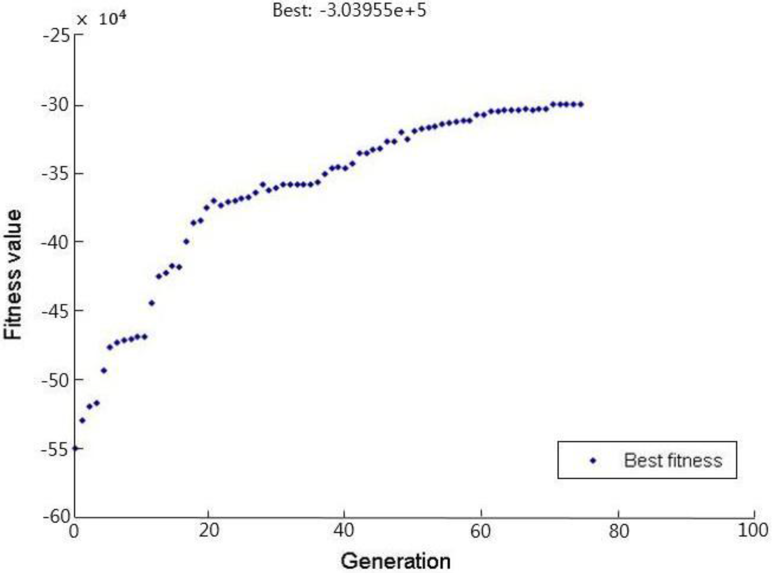
The GA recognizes that higher fitness is required; however, as the objective function was cost based it should be kept to minimum, and the fitness function had a negative value for the objective function as seen in Equation (8).
When the GA was executed, the individual with the best fitness was displayed as the generations moved on. The best fitness value rose and the evolutions were completed at generation 74 (
Figure 11). The evolution was rapid at the early and middle stages, before slowing at the later stages. This was attributed to the fact that it took time to choose the individuals of the parent generation and supplement lacking ones at an almost even probability as the solution set had good genes. Moreover, mutations sometimes degraded good genes [
42].
5.4. Optimization Result
5.4.1. Energy Optimization
In the energy optimization, without considering the cost, the model with a PV panel area ratio (X1) of 65%, skylight area ratio (X2) of 17.8% and a roof insulation thickness (X3) of 0.26 m used the least energy, with an energy consumption of 1,465,157 kWh.
5.4.2. Cost optimization
In the cost optimization, also considering the energy saving, the model with a PV panel area ratio (X1) of 1%, skylight area ratio (X2) of 17.8% and a roof insulation thickness (X3) of 0.26 m had the minimum LCC, with the cost standing at 3.03955 billion won.
5.5. Comparing the Energy Optimization Model and Cost Optimization Model
This study aimed to suggest a methodology to come up with a cost optimization model in the energy saving design. It also set out to show the importance of the cost optimization model by comparing it with the energy optimization model.
5.5.1. Comparison by optimal combination variables
The maximum 65% PV panel area ratio was used when only the energy was considered, within the PV panel area ratio range of 0 < X1 ≤ 0.65, while the minimum 1% was used when the energy and cost were considered together. When only the energy saving was considered, it is best to have a large PV panel area that can generate the maximum energy for the building. If the cost was also considered, however, keeping the panel area to a minimum resulted in the optimal model because the initial investment was greater than the savings resulting from the power generation. The 20-year analysis period for the building meant that the cost of the PV panels could not be recovered.
The optimization model that only considered the energy and the one which considered both the energy and cost presented the same value of the skylight area ratio at 17.8%, within the skylight area ratio range of 0 < X2 ≤ 0.85. If the skylight area could secure an average of 300 lux with only natural light, this was enough to save energy on the lighting. Since a skylight larger than this would cause energy losses, the appropriate skylight area ratio was 17.8%. The same result came out in the cost optimization because the operating cost saved from the energy optimization model was found to be greater than the initial investment saved with the skylight area ratio reduced to below 17.8%.
The optimization model that only considered energy and the one which considered both the energy and cost presented the same value of 0.26 m, within the roof insulation thickness range of 0.05 < X3 ≤ 0.26. As a thicker roof insulation would be more effective at saving energy when cooling or heating, the maximum value within the range would make the optimal model. As with the skylight area ratio, the maximum value within the range was found to be the most effective, saving on the operating cost rather than lowering the initial investment.
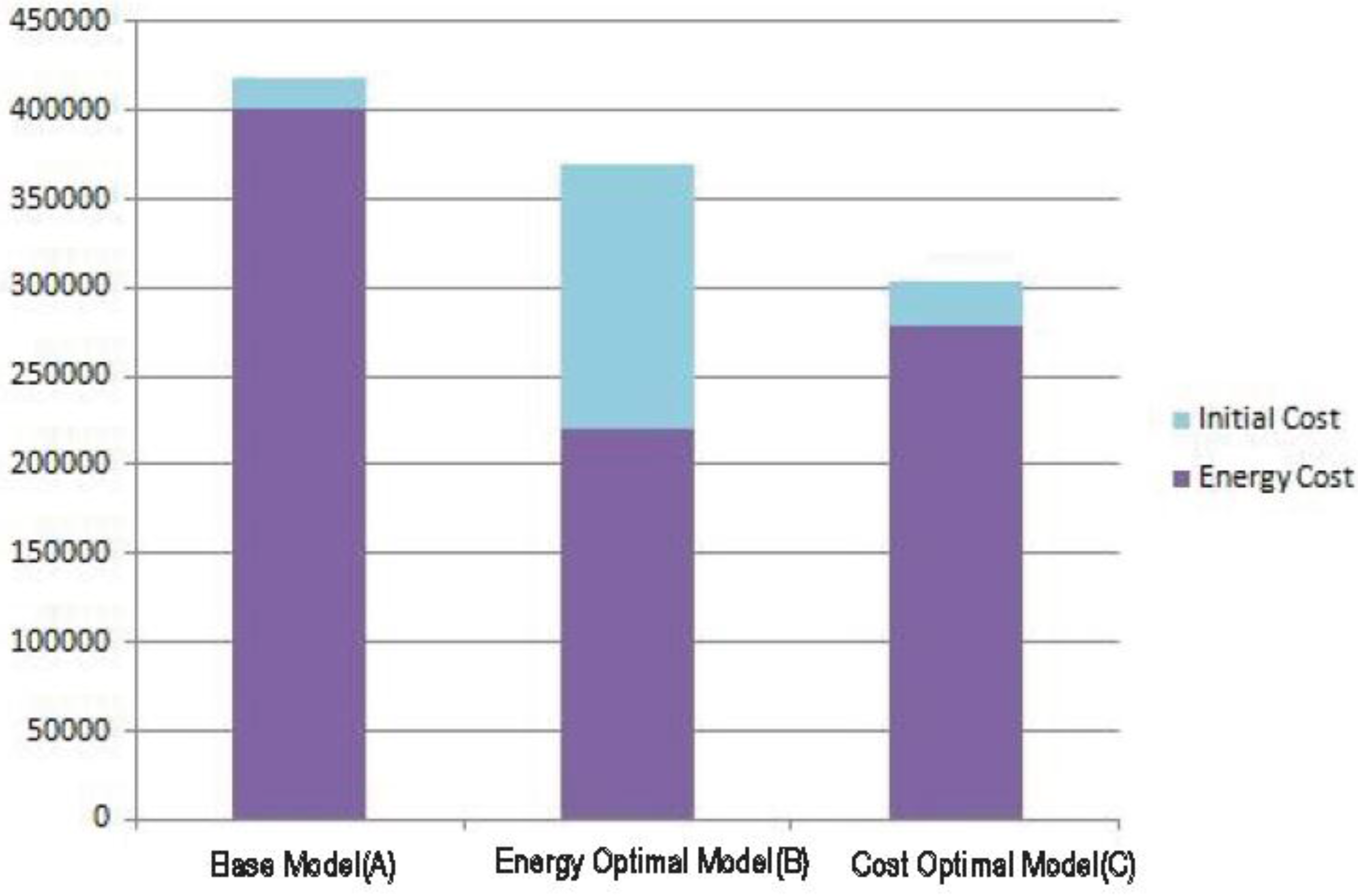
5.5.2. LCC result analysis
Calculation of the LCC of the original plan (
A), energy optimization model (
B) and cost optimization model (
C) showed that the energy cost was in the precedence order
A >
C >
B. Based on the LCC, however, the total cost order was
A >
B >
C. The energy optimization model could save more energy than the cost optimization model but did not consider cost, resulting in a greater initial investment and reducing the LCC by only 11.5% from the original plan. On the other hand, the cost optimization model saved less energy than the energy optimization model, though it did not incur an increase in the initial investment and could reduce the LCC by 27.3% compared to the original plan (
Figure 12) (
Table 5).
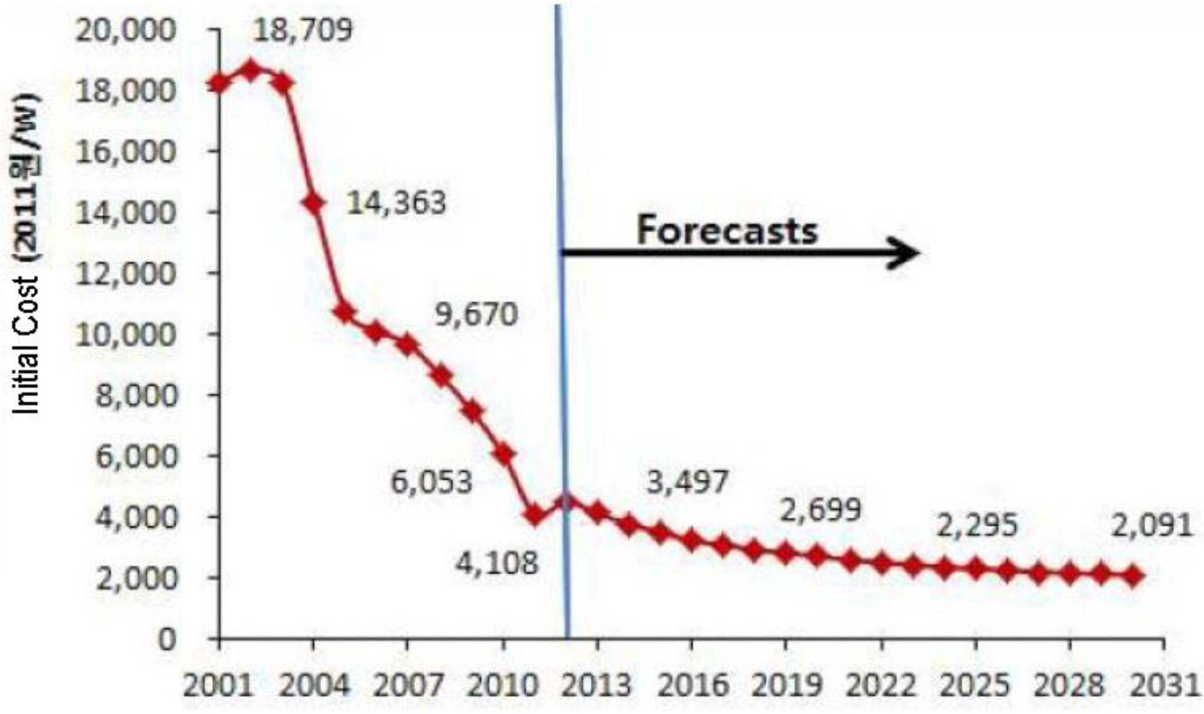
5.6. Cost Optimization Model Depending on the Initial Investment of the PV Panel
In the cost optimization model, not using the PV panels brought about the lowest LCC. However, technological development has brought down PV panel cost and it is expected to drop further in the future, meaning that the cost optimization model may not be correct with current technology. The unit price of the PV panels that should be adopted in the cost optimization model can be predicted based on panel price trends and an estimated price. In the cost optimization model, the PV panel price was designated as the fourth variable of
X4 in a range from 4108 won per watt in 2011 to 2091 won per watt in 2030. The PV panel price previously applied was from 2013. To account for the slight price rise from 2011 to 2012, the price was estimated in the range from 2012 to 2030, as can be seen in
Figure 13 (
Table 6). In the cost optimization, the panel cost becomes sufficiently reduced by 2024 when the PV panel costs 2317 won per watt (about 210,000 won/m
2) and the PV panel area ratio increases to 5%. After this point, the greater the PV panel area ratio is, the lower the LCC. Energy cost increases are different from general inflation when estimating the current value of the energy cost; therefore, if this were reflected in future studies, the PV panel would be adopted by the cost optimization model at an earlier stage.
6. Conclusions
This study suggested the use of an optimization technique as part of an optimization model for LCC economic feasibility analyses, aiming to apply energy saving techniques to the early building design stage. Different types of optimization techniques and the case studies describing their use were examined to select a method, and the resulting model produced the building energy simulation result as the LCC cost. Considering both the energy and cost, a unified structure was developed which performed energy simulations and cost optimization. Based on the energy saving techniques and a GA, a cost optimized process was introduced and case studies were performed on an industrial building to aid in further understanding the cost optimization model. A GA was applied that would function in locations with discontinuity and non-linearity, which are present in such cost optimizations.
A process to apply cost optimization to energy saving designs was proposed. To demonstrate the process in detail, an industrial building with high energy use was selected, as these have not been examined in detail previously. The model reflected the PV panel, skylight and roof insulation performances and dimming control of the lights as the energy saving items, and designated the PV panel area ratio (X1), skylight area ratio (X2) and roof insulation thickness (X3) as the design variables.
In addition to the cost optimization model case studies, different variable combinations and their LCC savings were illustrated by the energy optimization model. The combination of X1 = 1%, X2 = 17.8%, X3 = 0.26 m, was the optimum location found by the cost optimization model, and the differences with the energy optimization model were illustrated with that result X1 = 65%, X2 = 17.8%, X3 = 0.26 m. As the PV area ratio (X1) required a large initial investment compared with the energy saved, it was found to be an inappropriate design variable for the cost optimization model over the assumed life span of the building. On the other hand, the variables X2 and X3 were found to match both in the energy and cost optimization models. As a result, it was believed that the skylight area ratio and roof insulation thickness affected energy savings more than the initial investment. Similar to this, when the cost is considered with a combination of variables that is more sensitive to the initial investment than the energy saved, the cost optimization model must be used.
The cost optimization model can be a good alternative to the energy optimization model, which only focused on reducing the energy consumption, a less economical tactic. If the cost optimization model is suggested to investors who emphasize economic feasibility, the energy saving design can be recognized as a reasonable alternative from the building life cycle perspective. In spite of this, the LCC itself is based on a number of assumptions and it is difficult to estimate the exact cost because the cost data came from the statistics of a limited number of items. More studies should therefore be conducted on economic feasibility and optimization that can help to find energy saving combinations to rapidly minimize costs in the early design stage instead of providing an exact cost estimation.
Acknowledgments
This research was supported by the Basic Science Research Program through the National Research Foundation of Korea (NRF) funded by the Ministry of Science, ICT & Future Planning (NRF-2013R1A1A3013119).
Author Contributions
Haejin Kang conceived and designed the experiments; Hye Yeon Kim performed the experiments and analyzed the data.
Conflicts of Interest
The authors declare no conflict of interest.
References
- International Energy Agency (IEA). TASK 40/Annex 52 (2008). Towards Net Zero Energy Solar Buildings, IEASHC Task 40 and ECBCS Annex 52. 2011. Available online: http://www.ieashc.org/task40/index.html (accessed on 10 January 2011).
- European Council. Proposal for a directive of the European parliament and of the council on the energy performance of buildings, 2009. Available online: http://www.been-online.net/fileadmin/medias/downloads/beenetwork/news/2009nov/st16082.en09.pdf (accessed on 18 February 2016).
- Yong, J.K. Optimal Design of Residential Ventilation Systems Using Integration of Genetic Algorithm, Pareto Optimality and CONTAMW 2.4. Master Thesis, Sungkyunkwang University, Seoul, Korea, 2009. [Google Scholar]
- Kirkpatrick, S.; Gelatt, C.D.; Vecchi, M.P. Optimization by simulated annealing. Science 1983, 220, 671–680. [Google Scholar] [CrossRef] [PubMed]
- Hans-Georg, B.; Hans-Paul, S. Evolution Strategies: A Comprehensive Introduction. Nat. Comput. 2002, 1, 3–52. [Google Scholar]
- Holland, J. Adaptation in Natural and Artificial Systems; University of Michigan Press: Ann Arbor, MI, USA, 1975. [Google Scholar]
- Glover, F.; Laguna, M. Tabu Search; Kluwer: Boston, MA, USA, 1997. [Google Scholar]
- Storn, R.; Price, K. Differential evolution—A simple and efficient heuristic for global optimization over continuous spaces. J. Glob. Optim. 1975, 11, 341–359. [Google Scholar] [CrossRef]
- Logothetis, N.; Wynn, H.P. Quality through Design: Experimental Design, Off-Line Quality Control, and Taguchi’s Contributions; Oxford University Press: Oxford, UK, 1979; pp. 464–475. [Google Scholar]
- Kennedy, J.; Eberhart, R.C. Particle swarm optimization. In Proceedings of the IEEE International Conference on Neural Networks, Perth, WA, USA, 27 November–1 December 1995; pp. 1942–1948.
- Tuhus-Dubrow, D.; Krarti, M. Genetic-algorithm based approach to optimize building envelope design for residential buildings. Build. Environ. 2010, 45, 1574–1581. [Google Scholar] [CrossRef]
- Hamdy, M.; Hasan, A.; Siren, K. Applying a multi-objective optimization approach for design of low-emission cost-effective dwellings. Build. Environ. 2011, 46, 109–123. [Google Scholar] [CrossRef]
- Asadi, E.; da Silva, M.G.; Antunes, C.H.; Dias, L. A multi-objective optimization model for building retrofit strategies using TRNSYS simulations, GenOpt and MATLAB. Build. Environ. 2012, 56, 370–378. [Google Scholar] [CrossRef]
- Yi, H.; Srinivasan, R.S.; Braham, W.W. An integrated energy–emergy approach to building form optimization: Use of EnergyPlus, emergy analysis and Taguchi-regression method. Build. Environ. 2015, 84, 89–104. [Google Scholar] [CrossRef]
- Jung, B.R. A Study on Optimization Model of Time-Cost Trade-off Using Genetic Algorithm, Master’s Thesis, Angdong National University, Andong-si, Gyeongsangbuk-do, Korea, 2009. [Google Scholar]
- Woo, J.W. Sustainable Optimum Design Evaluation System Development by Environmental and Economical Efficiency of Life Cycle of the Apartment Houses. PhD. Thesis, Hanyang University, Seoul, Korea, 2011. [Google Scholar]
- Lee, D.C. Multi-Objective Optimization for Performance-Based Seismic Retrofit Considering Life Cycle Cost. Master’s Thesis, Yonsei University, Seoul, Korea, 2012. [Google Scholar]
- Bok, Y.J.; Tae, S.H.; Kim, R.H.; Roh, S.J. A Proposal on the Optimization Evaluate Method to Performance of Insulation Materials Considering Environmental and Economical Assessment. In Proceedings of the 2014 Conference of the Architectural Institute of Korea, Tongmyong University, Busan, Korea, 23–25 October 2014; pp. 623–624.
- Coley, D.A.; Schukat, S. Low-energy design: Combining computer-based optimisation and human judgement. Build. Environ. 2002, 37, 1241–1247. [Google Scholar] [CrossRef]
- Wang, J.J.; Jing, Y.Y.; Zhang, C.F.; Zhao, J.H. Review on multi-criteria decision analysis aid in sustainable energy decision-making. Renew. Sustain. Energy Rev. 2009, 13, 2263–2278. [Google Scholar] [CrossRef]
- Cai, Z.; Wang, Y.A. Multiobjective optimization-based evolutionary algorithm for constrained optimization. IEEE Trans. Evol. Comput. 2006, 10, 658–675. [Google Scholar] [CrossRef]
- Brinksa, P.; Kornadta, O.; Oly, R. Air infiltration assessment for industrial buildings. Energy Build. 2015, 86, 663–676. [Google Scholar] [CrossRef]
- Katunskyetl, D.; Korjenic, A.; Katunska, J.; Lopusniak, M. Analysis of thermal energy demand and saving in industrial building: A case study in Slovakia. Build. Environ. 2013, 67, 138–146. [Google Scholar] [CrossRef]
- Wang, X.; Kendrick, C.; Ogden, R.; Walliman, N.; Baiche, B. A case study on energy consumption and overheating for a UK industrial building with rooflights. Appl. Energy 2013, 104, 337–344. [Google Scholar] [CrossRef]
- Chen, Y.; Liu, J.; Pei, J.; Cao, X.; Chen, Q.; Jiang, Y. Experimental and simulation study on the performance of daylighting in an industrial building and its energy saving potential. Energy Build. 2014, 73, 184–191. [Google Scholar] [CrossRef]
- Munce, J.F. Industrial Architecture: An Analysis of International Building Practice; F.W. Dodge Corporation: New York, NY, USA, 1960; pp. 52–60. [Google Scholar]
- Eo, G.J. Study on the selection of insulation materials of prefab sandwich panel according to the types of factory building. Master’s Thesis, Graduate School of Architectural Engineering, Yonsei University, 2010. [Google Scholar]
- Asdrubali, F. Daylighting performance of saw tooth roofs of industrial buildings. Light. Res. Technol. 2003, 35, 343–359. [Google Scholar] [CrossRef]
- Leven, B.; Weber, C. Energy Efficiency in Innovative Industries: Application and Benefits of Energy Indicators in the Automobile Industry. In Proceedings of the American Council for an Energy-Efficient Economy: Summer Study on Energy Efficiency in Industry, Washington, DC, USA, 24–27 July 2001; pp. 67–75.
- Paroncini, M.; Calcagni, B. Comment on “Daylighting performance of sawtooth roofs of industrial buildings” by F Asdrubali. Light. Res. Technol. 2003, 35, 358–359. [Google Scholar] [CrossRef]
- Li, D.H.W.; Lam, J.C. Measurements of solar radiation and illuminance on vertical surfaces and daylighting implications. Renew. Energy 2000, 20, 389–404. [Google Scholar] [CrossRef]
- Joedicke, J. Shell Architecture, 3rd ed.; Karl Kramer: Stuttgart, Germany, 1963; pp. 1–10. [Google Scholar]
- Kuchta, M. Daylighting in American Industrial Architecture: Three Investigations. Master’s Thesis, Rice University, Houston, TX, USA, 1994. [Google Scholar]
- U.S. Department of Energy. Policies for A/C and Heating Temperature Set-Points in Municipal Facilities. Available online: http://www.eereblogs.energy.gov/tap/post/QA-Policies-for-AC-and-Heating-Temperature-Set-points-in-Municipal-Facilities.aspx (accessed on 19 December 2012).
- Galayda, J.; Yudelson, J. Inside Going Green: The Little Green Book of Corporate Sustainability; National Association of Electrical Distributors Education & Research Foundation, Inc.: St. Louis, MO, USA, 2009. [Google Scholar]
- Wright, J.A.; Loosemore, H.A.; Farmani, R. Optimization of building thermal design and control by multi-criterion genetic algorithm. Energy Build. 2002, 34, 959–972. [Google Scholar] [CrossRef]
- Wetter, M.; Wright, J. A comparison of deterministic and probabilistic optimization algorithms for nonsmooth simulation-based optimization. Build. Environ. 2004, 39, 989–999. [Google Scholar] [CrossRef]
- Mastrapostoli, E.; Karlessi, T.; et al. On the cooling potential of cool roofs in cold climates: Use of cool fluorocarbon coatings to enhance the optical properties and the energy performance of industrial buildings. Energy Build. 2014, 69, 417–425. [Google Scholar] [CrossRef]
- Chan, W.R.; Nazaroff, W.W.; Price, P.N.; Sohn, M.D.; Gadgil, A.J. Analyzing adatabase of residential air leakage in the United States. Atmos. Environ. 2005, 39, 3445–3455. [Google Scholar] [CrossRef]
- Jokisalo, J.; Kurnitski, J.; Korpi, M.; Kalamees, T.; Vinha, J. Building leakage, infiltra-tion, and energy performance analyses for Finnish detached houses. Build. Environ. 2009, 44, 377–387. [Google Scholar] [CrossRef]
- Pan, W. Relationships between air-tightness and its influencing factors of post-2006 new-build dwellings in the UK. Build. Environ. 2010, 45, 2387–2399. [Google Scholar] [CrossRef]
- Heras, M.R.; Jimenez, M.J.; et al. Energetic analysis of a passive solar design, incorporated in a courtyard after refurbishment, using an innovative cover component based in a sawtooth roof concept. Sol. Energy 2005, 78, 85–96. [Google Scholar] [CrossRef]
© 2016 by the authors; licensee MDPI, Basel, Switzerland. This article is an open access article distributed under the terms and conditions of the Creative Commons by Attribution (CC-BY) license (http://creativecommons.org/licenses/by/4.0/).


