
Thermo-Economic Analysis of Zeotropic Mixtures and Pure Working Fluids in Organic Rankine Cycles for Waste Heat Recovery †

Abstract
:1. Introduction
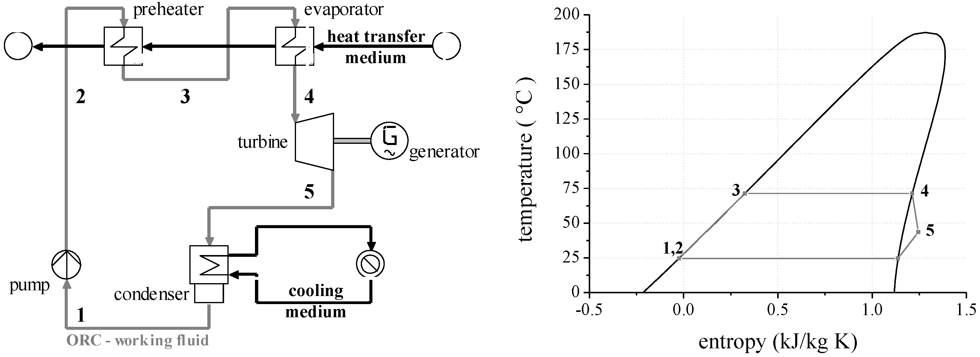
2. Methods
2.1. Exergy Analysis
2.2. Component Design and Economic Analysis
2.3. Exergy Costing
3. Results and Discussion
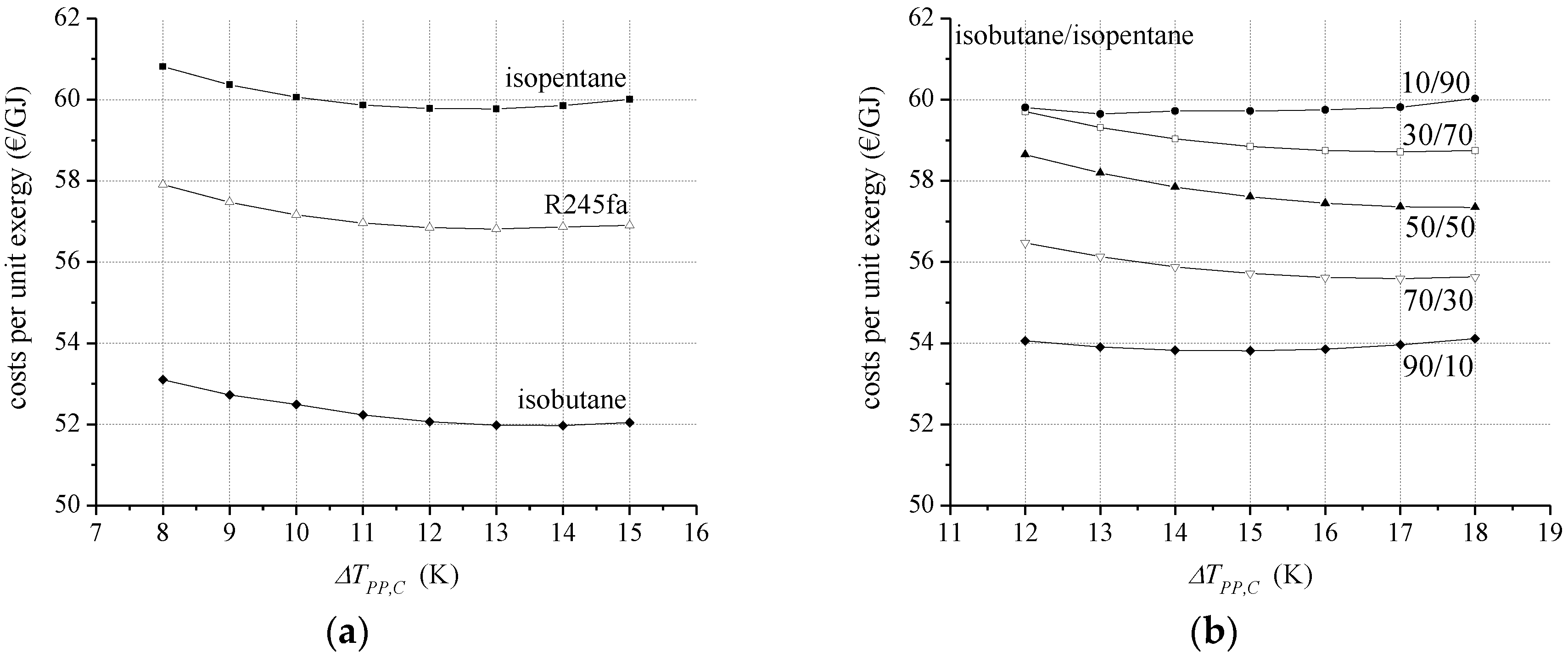
3.1. Identification of Cost-Efficient Design Parameters
3.2. Comparison of ORC Working Fluids
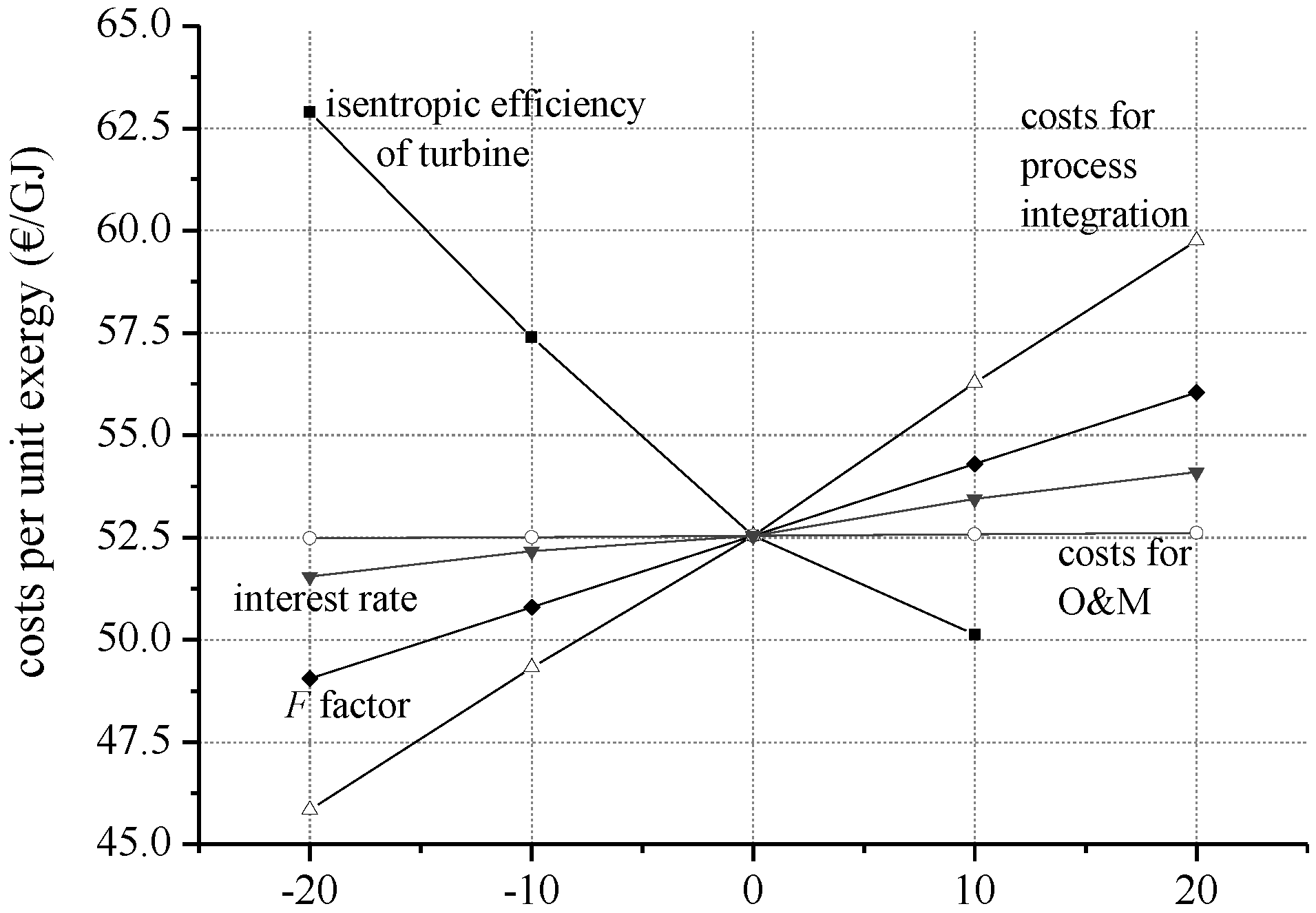
3.3. Sensitivity Analysis for Selected Boundary Conditions
4. Conclusions
Acknowledgments
Author Contributions
Conflicts of Interest
Abbreviations
| ORC | Organic Rankine Cycle |
Nomenclature
| A | heat transfer area | (m2) |
| c | costs per unit exergy | (€/GJ) |
| C | costs | (€) |
| cost rate | (€/h) | |
| D | diameter | (mm) |
| e | specific exergy | (kJ/kg) |
| exergy flow | (kW) | |
| F | correction factor | (-) |
| h | specific enthalpy | (kJ/kg) |
| K | constant | (-) |
| ṁ | mass flow | (kg/s) |
| Ns | specific speed | (-) |
| p | pressure | (bar) |
| P | power | (kW) |
| r | radius | (m) |
| rd | relative deviation | (%) |
| s | specific entropy | (kJ/(kgK)) |
| SIC | specific investment costs | (€/kW) |
| SP | size parameter | (-) |
| T | temperature | (°C) |
| U | overall heat transfer coefficient | (W/(m2K)) |
| Y | capacity/size parameter | (kW) or (m2) |
| cost rate | (€/h) | |
| α | heat transfer coefficient | (W/(m2K)) |
| ΔT | temperature difference | (K) |
| η | efficiency | (%) |
Subscript
| C | condenser |
| CI | capital investment |
| CM | cooling medium |
| D | destruction |
| E | evaporator |
| F | fuel |
| G | generator |
| HS | heat source |
| i | inner |
| in | inlet |
| is | isentropic |
| II | second law |
| k | k-th component |
| L | loss |
| LMTD | logarithmic mean temperature difference |
| log | logarithmic |
| m | mean |
| net | net |
| o | outer |
| out | outlet |
| O&M | operation and maintenance |
| P | product |
| PH | preheater |
| PP | pinch point |
| Pump | pump |
| s | specific |
| t | tube |
| tot | total |
| 0 | reference state |
Appendix A
R245fa
Isobutane
Isopentane
Isobutane/Isopentane
Appendix B
References
- Tchanche, B.F.; Lambrinos, G.; Frangoudakis, A.; Papadakis, G. Low-grade heat conversion into power using organic Rankine cycles—A review of various applications. Renew. Sustain. Energy Rev. 2011, 15, 3963–3979. [Google Scholar] [CrossRef]
- Angelino, G.; Di Paliano, P.C. Multicomponent Working Fluids for Organic Rankine Cycles (ORCs). Energy 1998, 23, 449–463. [Google Scholar] [CrossRef]
- Iqbal, K.Z.; Fish, L.W.; Starling, K.E. Advantages of using mixtures as working fluids in geothermal binary cycles. Proc. Okla. Acad. Sci. 1976, 56, 110–113. [Google Scholar]
- Demuth, O.J. Analyses of mixed hydrocarbon binary thermodynamic cycles for moderate temperature geothermal resources. In Proceedings of the Intersociety Energy Conversion Engineering Conference (IECEC), Atlanta, GA, USA, 9–14 August 1981.
- Borsukiewicz-Gozdur, A.; Nowak, W. Comparative analysis of natural and synthetic refrigerants in application to low temperature Clausius-Rankine cycle. Energy 2007, 32, 344–352. [Google Scholar] [CrossRef]
- Wang, X.D.; Zhao, L. Analysis of zeotropic mixtures used in low-temperature solar Rankine cycles for power generation. Sol. Energy 2009, 83, 605–613. [Google Scholar] [CrossRef]
- Chen, H.; Goswami, D.Y.; Rahman, M.M.; Stefanakos, E.K. A supercritical Rankine cycle using zeotropic mixture working fluids for the conversion of low-grade heat into power. Energy 2011, 36, 549–555. [Google Scholar] [CrossRef]
- Garg, P.; Kumar, P.; Srinivasan, K.; Dutta, P. Evaluation of isopentane, R-245fa and their mixtures as working fluids for organic Rankine cycles. Appl. Therm. Eng. 2013, 51, 292–300. [Google Scholar] [CrossRef]
- Dong, B.; Xu, G.; Cai, Y.; Li, H. Analysis of zeotropic mixtures used in high-temperature Organic Rankine cycle. Energy Convers. Manag. 2014, 84, 253–260. [Google Scholar] [CrossRef]
- Lecompte, S.; Ameel, B.; Ziviani, D.; Van Den Broek, M.; De Paepe, M. Exergy analysis of zeotropic mixtures as working fluids in Organic Rankine Cycles. Energy Convers. Manag. 2014, 85, 727–739. [Google Scholar] [CrossRef]
- Shu, G.; Gao, Y.; Tian, H.; Wei, H.; Liang, X. Study of mixtures based on hydrocarbons used in ORC (Organic Rankine Cycle) for engine waste heat recovery. Energy 2014, 74, 428–438. [Google Scholar] [CrossRef]
- Heberle, F.; Preißinger, M.; Brüggemann, D. Zeotropic mixtures as working fluids in Organic Rankine Cycles for low-enthalpy geothermal resources. Renew. Energy 2012, 37, 364–370. [Google Scholar] [CrossRef]
- Andreasen, J.G.; Larsen, U.; Knudsen, T.; Pierobon, L.; Haglind, F. Selection and optimization of pure and mixed working fluids for low grade heat utilization using organic rankine cycles. Energy 2014, 73, 204–213. [Google Scholar] [CrossRef] [Green Version]
- Angelino, G.; Colonna, P. Air cooled siloxane bottoming cycle for molten carbonate fuel cells. In Proceedings of the Fuel Cell Seminar, Portland, OR, USA, 30 October–02 November 2000; pp. 667–670.
- Weith, T.; Heberle, F.; Preißinger, M.; Brüggemann, D. Performance of Siloxane Mixtures in a High-Temperature Organic Rankine Cycle Considering the Heat Transfer Characteristics during Evaporation. Energies 2014, 7, 5548–5565. [Google Scholar] [CrossRef]
- Tempesti, D.; Fiaschi, D. Thermo-economic assessment of a micro CHP system fuelled by geothermal and solar energy. Energy 2013, 58, 45–51. [Google Scholar] [CrossRef]
- Astolfi, M.; Romano, M.C.; Bombarda, P.; Macchi, E. Binary ORC (Organic Rankine Cycles) power plants for the exploitation of medium–low temperature geothermal sources—Part B: Techno-economic optimization. Energy 2014, 66, 435–446. [Google Scholar] [CrossRef]
- Heberle, F.; Brüggemann, D. Thermoeconomic Analysis of Hybrid Power Plant Concepts for Geothermal Combined Heat and Power Generation. Energies 2014, 7, 4482–4497. [Google Scholar] [CrossRef]
- Calise, F.; Capuozzo, C.; Carotenuto, A.; Vanoli, L. Thermoeconomic analysis and off-design performance of an organic Rankine cycle powered by medium-temperature heat sources. Sol. Energy 2014, 103, 595–609. [Google Scholar] [CrossRef]
- Desai, N.B.; Bandyopadhyay, S. Thermo-economic analysis and selection of working fluid for solar organic Rankine cycle. Appl. Therm. Eng. 2016, 95, 471–481. [Google Scholar] [CrossRef]
- Quoilin, S.; Declaye, S.; Tchanche, B.F.; Lemort, V. Thermo-economic optimization of waste heat recovery Organic Rankine Cycles. Appl. Therm. Eng. 2011, 31, 2885–2893. [Google Scholar] [CrossRef]
- Imran, M.; Park, B.S.; Kim, H.J.; Lee, D.H.; Usman, M.; Heo, M. Thermo-economic optimization of Regenerative Organic Rankine Cycle for waste heat recovery applications. Energy Convers. Manag. 2014, 87, 107–118. [Google Scholar] [CrossRef]
- Quoilin, S.; Broek, M.V.D.; Declaye, S.; Dewallef, P.; Lemort, V. Techno-economic survey of Organic Rankine Cycle (ORC) systems. Renew. Sustain. Energy Rev. 2013, 22, 168–186. [Google Scholar] [CrossRef]
- Heberle, F.; Bassermann, P.; Preissinger, M.; Brüggemann, D. Exergoeconomic optimization of an Organic Rankine Cycle for low-temperature geothermal heat sources. Int. J. Thermodyn. 2012, 15, 119–126. [Google Scholar] [CrossRef]
- Heberle, F.; Brüggemann, D. Thermo-Economic Evaluation of Organic Rankine Cycles for Geothermal Power Generation Using Zeotropic Mixtures. Energies 2015, 8, 2097–2124. [Google Scholar] [CrossRef]
- Le, V.L.; Kheiri, A.; Feidt, M.; Pelloux-Prayer, S. Thermodynamic and economic optimizations of a waste heat to power plant driven by a subcritical ORC (Organic Rankine Cycle) using pure or zeotropic working fluid. Energy 2014, 78, 622–638. [Google Scholar] [CrossRef]
- Feng, Y.; Zhang, Y.; Li, B.; Yang, J.; Shi, Y. Sensitivity analysis and thermoeconomic comparison of ORCs (organic Rankine cycles) for low temperature waste heat recovery. Energy 2015, 82, 664–677. [Google Scholar] [CrossRef]
- Woudstra, N.; van der Stelt, T.P. Cycle-Tempo: A Program for the Thermodynamic Analysis and Optimization of Systems for the Production of Electricity, Heat and Refrigeration; Energy Technology Section, Delft University of Technology: Delft, The Netherlands, 2002. [Google Scholar]
- Lemmon, E.W.; Huber, M.L.; McLinden, M.O. Physical and Chemical Properties Division. In NIST Standard Reference Database 23—Version 9.1; National Institute of Standards and Technology: Boulder, CO, USA, 2013. [Google Scholar]
- Heberle, F.; Jahrfeld, T.; Brüggemann, D. Thermodynamic Analysis of Double-Stage Organic Rankine Cycles for Low-Enthalpy Sources based on a Case Study for 5.5 MWe Power Plant Kirchstockach (Germany). In Proceedings of the World Geothermal Congress, Melbourne, Australia, 19–25 April 2015.
- ORC systems—Bosch KWK Systeme. Available online: http://www.bosch-kwk.de/en/solutions/bosch-kwk-systeme-orc-systems/ (accessed on 22 February 2016).
- Bejan, A.; Tsatsaronis, G.; Moran, M. Thermal Design and Optimization; John Wiley & Sons: New York, NY, USA, 1996. [Google Scholar]
- Turton, R.; Bailie, R.C.; Whiting, W.B. Analysis, Synthesis and Design of Chemical Processes, 2nd ed.; Prentice Hall: Old Tappan, NJ, USA, 2003. [Google Scholar]
- Ulrich, G.D.; Vasudevan, P.T. Chemical Engineering—Process Design and Economics; John Wiley & Sons: New York, NY, USA, 2004. [Google Scholar]
- Stephan, P.; Kabelac, S.; Kind, M.; Martin, H.; Mewes, D.; Schaber, K. VDI Heat Atlas; Springer Verlag: Berlin, Germany, 2010. [Google Scholar]
- Kern, D.Q. Process Heat Transfer; McGraw-Hill: New York, NY, USA, 1950. [Google Scholar]
- Shah, M.M.; Sekulic, D.P. Heat Exchanger Design Procedures, in Fundamentals of Heat Exchanger Design; John Wiley & Sons: Hoboken, NJ, USA, 2003. [Google Scholar]
- Sieder, E.N.; Tate, G.E. Heat transfer and pressure drop of liquids in tubes. Ind. Eng. Chem. 1936, 28, 1429–1435. [Google Scholar] [CrossRef]
- Steiner, D. Wärmeübertragung beim Sieden gesättigter Flüssigkeiten (Abschnitt Hbb). In VDI-Wärmeatlas; Springer Verlag: Berlin, Germany, 2006. [Google Scholar]
- Schlünder, E.U. Heat transfer in nucleate boiling of mixtures. Int. Chem. Eng. 1983, 23, 589–599. [Google Scholar]
- Shah, M.M. A general correlation for heat transfer during film condensation inside pipes. Int. J. Heat Mass Transf. 1979, 22, 547–556. [Google Scholar] [CrossRef]
- Silver, R.S. An approach to a general theory of surface condensers. Proc. Inst. Mech. Eng. Part 1 1964, 179, 339–376. [Google Scholar]
- Bell, J.; Ghaly, A. An approximate generalized design method for multicomponent/partial condensers. AIChe Symp. Ser. Heat Transf. 1973, 69, 72–79. [Google Scholar]
- Tsatsaronis, G.; Winhold, M. Exergoeconomic analysis and evaluation of energy-conversion plants—I. A new general methodology. Energy 1985, 10, 69–80. [Google Scholar] [CrossRef]
- Klonowicz, P.; Heberle, F.; Preißinger, M.; Brüggemann, D. Significance of loss correlations in performance prediction of small scale, highly loaded turbine stages working in Organic Rankine Cycles. Energy 2014, 72, 322–330. [Google Scholar] [CrossRef]


| Parameter | Value |
|---|---|
| mass flow rate of heat source ṁHS | 10 kg/s |
| outlet temperature of heat source THS,in | 80 °C |
| inlet temperature of cooling medium TCM,in | 15 °C |
| temperature difference of cooling medium ΔTCM | 15 °C |
| maximal ORC process pressure p2 | 0.8∙pcrit |
| isentropic efficiency of feed pump ηi,P | 75% |
| isentropic efficiency of turbine ηis,T | 80% |
| efficiency of generator ηG | 98% |
| Component | Y; Unit | K1 | K2 | K3 |
|---|---|---|---|---|
| pump (centrifugal) | kW | 3.3892 | 0.0536 | 0.1538 |
| heat exchanger (floating head) | m2 | 4.8306 | −0.8509 | 0.3187 |
| heat exchanger (air cooler) | m2 | 4.0336 | 0.2341 | 0.0497 |
| turbine (axial) | kW | 2.7051 | 1.4398 | −0.1776 |
| Heat Exchanger | Tube Side |
|---|---|
| preheater | Sieder and Tate [38] |
| evaporator (pure working fluid) | Steiner [39] |
| evaporator (zeotropic mixture) | Schlünder [40] |
| condenser (pure working fluid) | Shah [41] |
| condenser (zeotropic mixture) | Silver, Bell, and Ghaly [42,43] |
| Parameter | Value |
|---|---|
| Lifetime n | 20 years |
| Interest rate ir | 4.0% |
| Annual operation hours | 7500 h/year |
| Cost rate for operation and maintenance CO&M | 0.02∙CI |
| Costs for process integration CPI | 0.2∙CORC,MC |
| Power requirements of the air-cooling system | 5 kWe/MWth |
| Electricity price €/kWh | 0.08 €/kWh |
| Parameter | Isobutane | R245fa | Isopentane | Isobutane/Isopentane |
|---|---|---|---|---|
| APH (m2) | 173.2 | 100.0 | 90.8 | 108.1 |
| AE (m2) | 123.1 | 118.1 | 118.6 | 112.8 |
| AC (m2) | 747.1 | 821.7 | 856.0 | 785.0 |
| PG (kW) | 387.8 | 345.9 | 331.0 | 366.4 |
| PPump (kW) | 60.1 | 21.6 | 12.1 | 41.4 |
| ΔTPP,E (K) | 1.2 | 1.0 | 1.0 | 2.0 |
| ΔTPP,C (K) | 14.0 | 13.0 | 13.0 | 15.0 |
| ηII (%) | 30.3 | 30.0 | 29.4 | 30.0 |
| SICMC (€/kW) | 1161.9 | 1270.1 | 1336.2 | 1203.0 |
| SICTM (€/kW) | 7343.2 | 8027.3 | 8445.0 | 7602.7 |
| LCOE (€/MWh) | 106.5 | 107.9 | 110.3 | 106.0 |
| cp,tot (€/GJ) | 52.0 | 56.8 | 59.8 | 53.8 |
| Parameter | Isobutane | R245fa | Isopentane | Isobutane/Isopentane |
|---|---|---|---|---|
| ηi,T (%) | 78.5 | 80.2 | 80.6 | 78.8 |
| rdηi,T (%) | 1.9 | 0.3 | 0.8 | 1.5 |
| SP (-) | 0.0486 | 0.0729 | 0.0820 | 0.0508 |
| Dm (mm) | 130.5 | 195.7 | 220.1 | 136.7 |
| cp,tot (€/GJ) | 52.2 | 56.7 | 59.1 | 54.0 |
| rdcp,tot (%) | 0.4 | 0.2 | 1.3 | 0.4 |
| Cost Estimation Method | cp,tot (€/GJ) | LCOE (€/MWh) | SICTM (€/kW) |
|---|---|---|---|
| Fcosts = 6.32 | 52.0 | 106.5 | 7332.5 |
| Fcosts = 4.31 | 46.4 | 83.2 | 5000.5 |
| CTM,Turton | 40.5 | 58.7 | 2554.7 |
| CTM,Ulrich | 43.7 | 71.9 | 3875.1 |
© 2016 by the authors; licensee MDPI, Basel, Switzerland. This article is an open access article distributed under the terms and conditions of the Creative Commons by Attribution (CC-BY) license (http://creativecommons.org/licenses/by/4.0/).
Share and Cite
Heberle, F.; Brüggemann, D. Thermo-Economic Analysis of Zeotropic Mixtures and Pure Working Fluids in Organic Rankine Cycles for Waste Heat Recovery. Energies 2016, 9, 226. https://doi.org/10.3390/en9040226
Heberle F, Brüggemann D. Thermo-Economic Analysis of Zeotropic Mixtures and Pure Working Fluids in Organic Rankine Cycles for Waste Heat Recovery. Energies. 2016; 9(4):226. https://doi.org/10.3390/en9040226
Chicago/Turabian StyleHeberle, Florian, and Dieter Brüggemann. 2016. "Thermo-Economic Analysis of Zeotropic Mixtures and Pure Working Fluids in Organic Rankine Cycles for Waste Heat Recovery" Energies 9, no. 4: 226. https://doi.org/10.3390/en9040226