Article

Anti-Windup Load Frequency Controller Design for Multi-Area Power System with Generation Rate Constraint

1
Institute of Advanced Technology, Nanjing University of Posts and Telecommunications, Nanjing 210023, China
2
College of Automation, Nanjing University of Posts and Telecommunications, Nanjing 210023, China
*
Author to whom correspondence should be addressed.
Energies 2016, 9(5), 330; https://doi.org/10.3390/en9050330
Submission received: 25 December 2015 / Revised: 21 April 2016 / Accepted: 21 April 2016 / Published: 29 April 2016
(This article belongs to the Special Issue Electric Power Systems Research)

Abstract

:
To deal with the problem of generation rate constraint (GRC) during load frequency control (LFC) design for a multi-area interconnected power system, this paper proposes an anti-windup controller design method. Firstly, an H dynamic controller is designed to obtain robust performance of the closed-loop control system in the absence of the GRC. Then, an anti-windup compensator (AWC) is formulated to restrict the magnitude and rate of the control input (namely power increment) in the prescribed ranges so that the operation of generation unit does not exceed the physical constraints. Finally, the anti-windup LFC is tested on the multi-area interconnected power systems, and the simulation results illustrate the effectiveness of the proposed LFC design method with GRC.

Graphical Abstract

1. Introduction

In a multi-area interconnected power system, it is important for the system’s operation to keep the active power balance and regulate the tie-line power at the scheduled value. Load frequency control (LFC) plays several key roles in the active power control of the interconnected power system [1,2], such as counteracting the load fluctuation, stabilizing the system frequency, regulating the tie-line power, and narrowing the area control error (ACE). Thus, the LFC is vital for the security and stability of power system.
On the issue of LFC design for a power system, an amount of work has been done in recent years. The conventional LFC usually adopts the proportional-integral (PI)-type controller because it has simpler structure and fewer tuning parameters. However, this kind of controller has shortcomings in terms of coping with the operating point change and the load disturbance, since they are designed on nominal operating points with fixed parameters. In order to obtain better performance of the PI-type LFC, the parameter optimization methods of the PI-type controller are proposed in [3,4,5]. To enhance the robustness and reliability of the control system, some fuzzy-logic-based LFC methods are introduced in [6,7,8,9]. In addition, some advanced control technologies are utilized to improve LFC performance, such as sliding mode methods [10,11,12], optimal or suboptimal feedback control methods [13,14,15,16], and robust control methods [17,18,19]. Considering the delay in the open communication network, the authors in [20,21,22] analyze the influence of time delay on the LFC and present the relevant controller design methods. To guarantee compliance with the control performance standards (CPS) of North American Electric Reliability Council (NERC) and reduce wear and tear of generators, a decentralized model predictive control method is used to deal with the LFC problem [23]. For accommodating unexpected load change and faults, the supervisory control strategies in [24,25] are proposed to solve the load and frequency set-point problem. It is well known that due to physical limitations, generation units have inherent generation rate constraints (GRC), such as ramp rate constraints and upper-lower bound constraints. If GRC is not considered adequately in LFC design, the controller will not yield excellent performances, and even the closed-loop system stability may be destroyed under disturbances [26,27,28]. In the aforementioned research work, some studies make tentative consideration on the GRC problem. In [1,7,8,12], GRC is considered in the simulation, but neglected in the controller design. Therefore, the validity of these methods to deal with GRC lacks theoretical support. Towards LFC design with GRC, the extended integral control method in [26], the biased PI dual mode control method in [27], the Type-2 fuzzy approach in [28], and the anti-GRC PI-type controller in [29,30] are adopted to deal with the GRC problem. Unfortunately, the strict mathematical proof in the above methods is still absent.
Focusing on the LFC design with GRC, this paper proposes an anti-windup LFC design method for the multi-area interconnected power system. The designed LFC consists of a robust H controller and an anti-windup compensator (AWC). The former is used to guarantee the stability and robustness of the closed-loop system without constraints, and the latter takes charge of restricting the rate and magnitude of control input in the prescribed ranges to make the operation of generation unit meet the GRC requirement. For verifying the proposed method, several multi-area interconnected power systems are employed for testing. The comparative simulation results show that the performances of the LCF are improved by the design method of this paper.

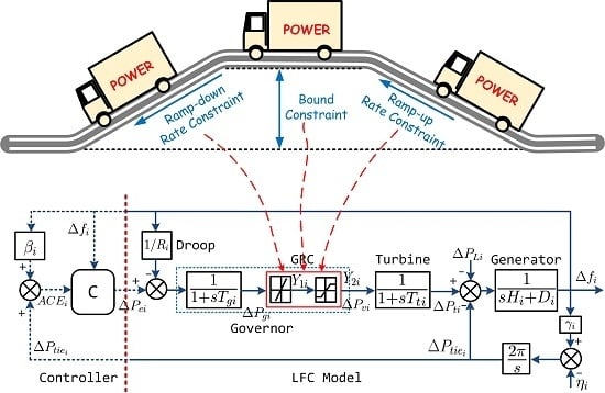
2. Load Frequency Control Model

The large interconnected power system is usually partitioned into several areas for management and control. Generally, for reducing the difficulty in the LFC design, each area in the LFC model is simplified to be an equivalent generator with a turbine and a governor shown in Figure 1. The dynamics of the generator, the turbine and the governor are described by three first-order inertial processes, respectively. In addition, since the generation unit has the physical operation limitations, the LFC model includes the GRC, namely the ramp rate and the upper-lower bound constraints of the generation units. As one knows, the GRC may generate adverse impact on the LFC performances if the GRC is not considered sufficiently in LFC design.
The GRC of LFC model shown in Figure 1 includes the magnitude and rate saturation of the states. This kind of state saturation nonlinearity causes much difficulty in controller design.
Remark 1. 
For a real power system, we know the fact that the generation unit will operate in the linear region (without touching the saturation bounds), if the power increment is limited in the magnitude and rate ranges appropriately. In other words, the generation unit can meet its GRC when the proper rate and magnitude constraints are imposed on the control signal of the LFC. Based on the above fact, the LFC design with GRC can be solved through dealing with the problem on the controller synthesis subject to the magnitude and rate saturation of the control. Assuming that the deigned controller makes the generation unit operate in the linear region, the nonlinear GRC of the LFC model can be removed, and thus the original LFC model can be modified into a new one as shown in Figure 2.
According to the LFC dynamic model diagram shown in Figure 2, the state-space LFC model can be written as:
Δ f ˙ i = 1 H i Δ P t i Δ P L i Δ P tie i D i Δ f i Δ P ˙ t i = 1 T t i ( Δ P t i Δ P g i ) Δ P ˙ g i = 1 T g i ( Δ P g i Δ P c i + 1 R i Δ f i ) Δ P ˙ tie i = γ i Δ f i η i I ˙ A C E i = A C E i = β i Δ f i + Δ P tie i y i 1 = Δ f i y i 2 = A C E i = β i Δ f i + Δ P tie i y i 3 = I A C E i
where γ i = j = 1 , j i N T i j ; η i = j = 1 , j i N T i j Δ f j ; f i denotes the system frequency; P t i denotes the turbine power; P g i denotes the governor valve; P c i denotes the governor power setpoint; P L i denotes the load demand; P tie i denotes the net tie-line power; A C E i denotes the area control error; I A C E i denotes the integral of A C E i ; Δ denotes the deviation from normal value; β i denotes the frequency bias coefficient; R i denotes the droop coefficient; T g i denotes the governor time constant; T t i denotes the turbine time constant; H i denotes the area aggregate inertia constant; D i denotes the area load damp constant; and T i j denotes the tie-line synchronizing coefficient.
Usually, we focus on the frequency deviation, the ACE and the control energy cost when evaluating the LFC performances. Thus, the controlled variables z for the H control design are selected as follows:
z i 1 = Δ f i z i 2 = I A C E i z i 3 = Δ P c i
For convenience, by defining the state variables x = [ Δ f i , Δ P t i , Δ P g i , Δ P tie i , I A C E i ] T R 5 , the control variable u = Δ P c i R 1 , the output variables y = [ y i 1 , y i 2 , y i 3 ] T R 3 , the controlled variables z = [ z i 1 , z i 2 , z i 3 ] T R 3 , and the disturbance variables d = [ Δ P L i , η i ] T R 2 , the state-space model P consisting of Equations (1) and (2) can be rewritten as:
P : x ˙ = A x + B u u + B d d y = C y x + D yu u + D yd d z = C z x + D zu u + D zd d
where:
A = D i H i 1 H i 0 1 H i 0 0 1 T t i 1 T t i 0 0 1 R i T g i 0 1 T g i 0 0 γ i 0 0 0 0 β i 0 0 1 0 ; B u = 0 0 1 T g i 0 0 ; B d = 1 H i 0 0 0 0 0 0 1 0 0
C y = 1 0 0 0 0 β i 0 0 1 0 0 0 0 0 1 ; D yu = 0 0 0 ; D yd = 0 0 0 0 0 0
C z = 1 0 0 0 0 0 0 0 0 1 0 0 0 0 0 ; D zu = 0 0 1 ; D zd = 0 0 0 0 0 0
The control input with rate and magnitude saturations shown in Figure 2 can be defined as:
u = s a t m ( φ ) = m ¯ , φ > m ¯ φ , m ̲ φ m ¯ m ̲ , φ < m ̲ φ ˙ = s a t r ( μ ) = r ¯ , μ > r ¯ μ , r ¯ μ r ¯ r ̲ , μ < r ̲
where s a t ( · ) denotes saturation function, [ m ̲ , m ¯ ] and [ r ̲ , r ¯ ] denote the magnitude bound and the rate bound, respectively.

3. Anti-Windup Load Frequency Controller Design

In this section, we design the LFC to ensure that the control input never exceeds the magnitude limit and the rate limit to meet the GRC. Based on the LFC model P , the anti-windup schemes [31,32] are employed to synthesize the LFC in the following subsections.

3.1. Original H Controller Design

According to the anti-windup scheme, a robust H controller is designed on the basis of the LFC model P in absence of the control input saturation in advance. Assuming that the system ( A , B u , C y ) is controllable and observable, we can design an H dynamic controller C ¯ with the following form:
C ¯ : x ˙ c ¯ = A c ¯ x c ¯ + B c ¯ u c ¯ y c ¯ = C c ¯ x c ¯ + D c ¯ u c ¯
where x c ¯ R 5 are the state variables of the controller; u c ¯ R 3 are the input variables of the controller (the measured variables of P : u c ¯ = y ); y c ¯ R 1 is the output variable of the controller (the control input variable of P : y c ¯ = u ); and A c ¯ , B c ¯ , C c ¯ , D c ¯ are the constant matrices with appropriate dimension.
Since the robust H design method is well-known, we do not intend to repeat them. If the detailed introduction of the method is needed, one can refer to the literatures [33,34]. In this paper, we use the MATLAB/Robust Linear Matrix Inequality (LMI) Control Box [35] to solve the robust controller C ¯ directly. Here, it is assumed that the closed-loop system consisting of P and C ¯ is well posed and gains the prescribed H performance without consideration of the control input saturations.

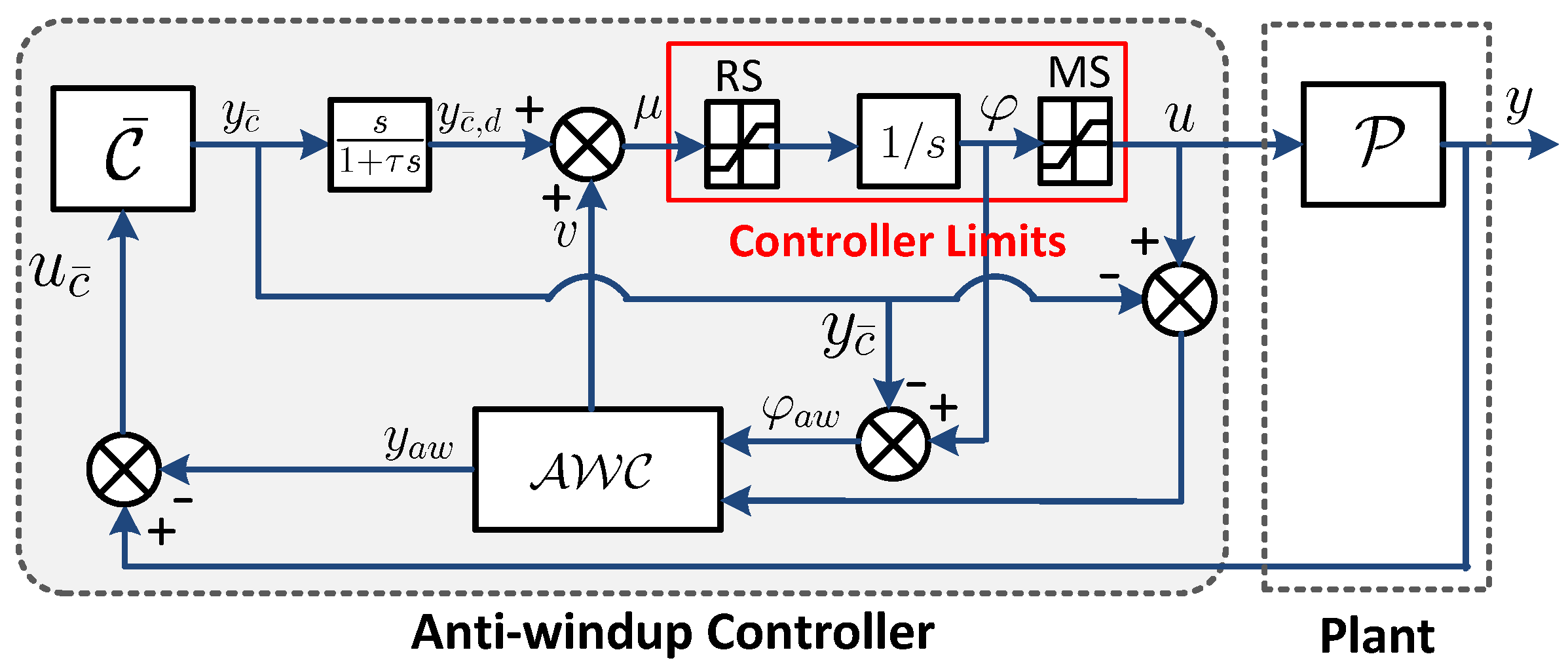
3.2. Anti-Windup Compensator Design

To tackle the magnitude and rate saturations of the control input, we borrow the anti-windup control scheme [32] shown in Figure 3.
In the anti-windup control approach, it is needed to compute the first-order derivative of the controller output y c ¯ . Here, the differentiator s is replaced by a linear filter s 1 + τ s with a sufficiently small constant τ , considering that the controller output may be not strictly proper. The modified controller consists of the original controller C ¯ and the filter s 1 + τ s can be expressed as:
C : x ˙ c = A c x c + B c u c y c = C c x c + D c u c
where x c = [ x c ¯ T , x f ] T R 6 are the modified controller states; x f R 1 are the filter states; u c = u c ¯ R 1 is the modified controller input; y c = [ y c ¯ , y c ¯ , d ] T R 2 are the modified controller outputs; y c ¯ , d R 1 denote approximate derivatives of y c ¯ ; and the parameter matrices of C are:
A c = A c ¯ 0 C c ¯ τ 1 τ , B c = B c ¯ D c ¯ τ , C c = C c ¯ 0 C c ¯ τ 1 τ , D c = D c ¯ D c ¯ τ
In Figure 3, the AWC is designed to cope with the controller limits. The AWC is formulated as follows:
AWC : x ˙ aw = A x aw + B u ( u y c ¯ ) y aw = C y x aw + D yu ( u y c ¯ ) z aw = C z x aw + D zu ( u y c ¯ ) v = K aw x aw φ aw
where x aw R 5 are the AWC states; y aw R 3 are the AWC output; ( u y c ¯ ) and φ aw = ( φ y c ¯ ) serve as the AWC input; z aw R 3 are the AWC controlled variables; v R 1 is the stabilizing signal which needs to be designed; and K aw R 1 × 6 is the gain matrix.
The plant Equation (3), the control input limitation Equation (4), the modified Controller Equation (6), and the AWC Equation (7) are interconnected by the following relationship:
u c = y y aw , μ = y c ¯ , d + v , φ aw = φ y c ¯
From the interconnection diagram shown in Figure 3, by defining the coordinate ( x , x c , x aw , φ aw ) = ( x x aw , x c , x aw , φ y c ¯ ) , after some derivations, we can obtain the equivalent expression of the whole closed-loop system as follows:
x ˙ = A x + B u y c ¯ + B d d y = C y x + D yu y c ¯ + D yd d z = C z x + + D zu y c ¯ + D zd d x ˙ c = A c x c + B c y y c = C c x c + D c y
x ˙ aw = A x aw + B u s a t m ( φ aw + y c ¯ ) y c ¯ φ ˙ aw = s a t r K aw x aw φ aw + y c ¯ , d y c ¯ , d z aw = C z x aw + D zu s a t m ( φ aw + y c ¯ ) y c ¯
where y = y y aw ; z aw = z z denotes the mismatch between the desirable performance output z of the modified closed-loop system Equations (3), (4) and (6) and the actual performance output z of the anti-windup closed-loop system Equations (3), (4), (6) and (7).
Theorem 1. 
Given the anti-windup closed-loop system Equations (3), (4), (6) and (7), if x aw ( 0 ) = 0 and φ ( 0 ) = y c ¯ ( 0 ) , then the control input u of the plant never exceeds the magnitude and rate saturation bounds. Moreover, if the K aw selection guarantees the asymptotic stability of the subsystem Equation (9b), then the following conclusions hold [31,32,36]:
  • Given any response of the modified closed-loop system Equations (3), (4) and (6) such that y c ¯ = s a t m ( y c ¯ ) and y c ¯ , d = s a t r ( y c ¯ , d ) for all t, then z = z for all t, namely, the response of the anti-windup closed-loop system coincides with the response of the modified closed-loop system;
  • The origin of the anti-windup closed-loop system is asymptotically stable.
Remark 2. 
(1) Under the initial conditions: x aw ( 0 ) = 0 and φ ( 0 ) = y c ¯ ( 0 ) , obviously, the control input u meets the magnitude and the rate constraints since they are prescribed by two saturation functions; (2) If the gain matrix K aw keeps the subsystem Equation (9b) stable under the foregoing initial conditions, we know that the variables x aw = 0 , φ aw = 0 , and v = 0 , thus z aw = C z x aw + D zu s a t m ( φ aw + y c ¯ ) y c ¯ = D zu s a t m ( y c ¯ ) y c ¯ = 0 with the given assumption y c ¯ = s a t m ( y c ¯ ) for all t, so z = z for all t is obtained based on the definition z aw = z z . (3) Given that K aw guarantees the asymptotic stability of subsystem Equation (9b), it can be known that x aw 0 , φ aw 0 , v 0 , y c ¯ s a t m ( y c ¯ ) , and y c ¯ , d s a t r ( y c ¯ , d ) from Equation (9b), then the magnitude and rate saturations of the control input are ignored, and the differentiator s / ( 1 + τ s ) offsets the integrator 1 / s in the control loop shown Figure 3, thus the asymptotic stability of the anti-windup closed-loop system is guaranteed by the original robust H controller c ¯ .
The proof of the above theorem is omitted in this paper, since it has been presented in the literature [31,32,36] in detail. According to the theorem, the key step for synthesizing the anti-windup controller is to design the gain matrix K aw to keep the subsystem Equation (9b) stable. In terms of the recipe in [32], the gain matrix K aw is selected to stabilize the following dynamic model:
x ˙ aw φ ˙ aw = A B u 0 0 + 0 I K aw x aw φ aw
Here, the LQR method can be used to obtain K aw . Obviously, K aw stabilizing the dynamic model Equation (10) implies the asymptotic stability of Equation (9b), when y c , y c , d and v are sufficiently small (not to cause the saturation nonlinearity).
Remark 3. 
From the control diagram shown in Figure 3, we can see that the AWC is inserted between the robust H controller c ¯ and the plant P , thus the closed-loop system has a typical structure of the cascade control system. To obtain satisfied performances of the closed-loop system, it is required that the response time of the AWC in inner loop should be much shorter than that of the H controller c ¯ in outer loop. Thus, when solving the gain matrix K aw based on the dynamic model Equation (10), we need to take the above requirement into account.

4. Case Study

To test the proposed LFC design method, firstly a typical two-area interconnected power system shown in Figure 4 is selected to make simulations. In the test system, each area is represented by a equivalent generation unit with a turbine and a governor. For simplicity, it is assumed that the two areas are identical, and the corresponding parameters are as [29]: T g 1 = T g 2 = 0 . 08 ( s ) , T t 1 = T t 2 = 0 . 3 ( s ) , H 1 = H 2 = 0 . 1667 ( pu . s ) , D 1 = D 2 = 0 . 0083 ( pu / Hz ) , T 12 = T 21 = γ 1 = γ 2 = 0 . 545 ( pu / Hz ) , R 1 = R 2 = 2 . 4 ( Hz / pu ) , β 1 = β 2 = 0 . 425 ( pu / Hz ) , rate constraint ( pu / s ) : [ 0 . 0017 , 0 . 0017 ] , magnitude constraint ( pu ) : [ 0 . 1 , 0 . 1 ] . Then, based on the above parameters, the two-area system shown in Figure 4 is modified into a single-area system and two three-area systems in the following simulations.
In this section, the proposed method for LFC design is compared with the methods proposed by Tan [29] and Anwar [30] for three scenarios with different load disturbances.

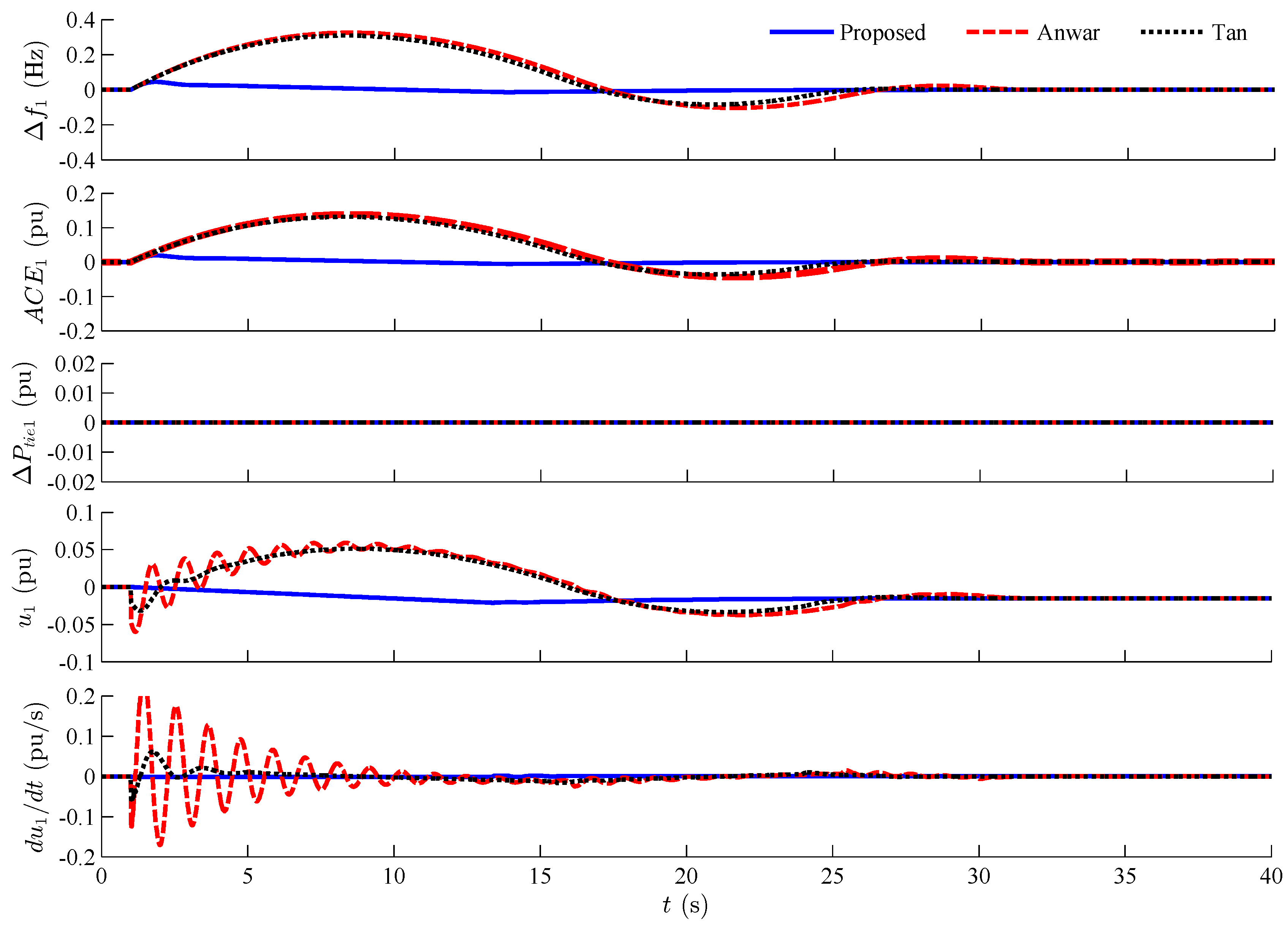
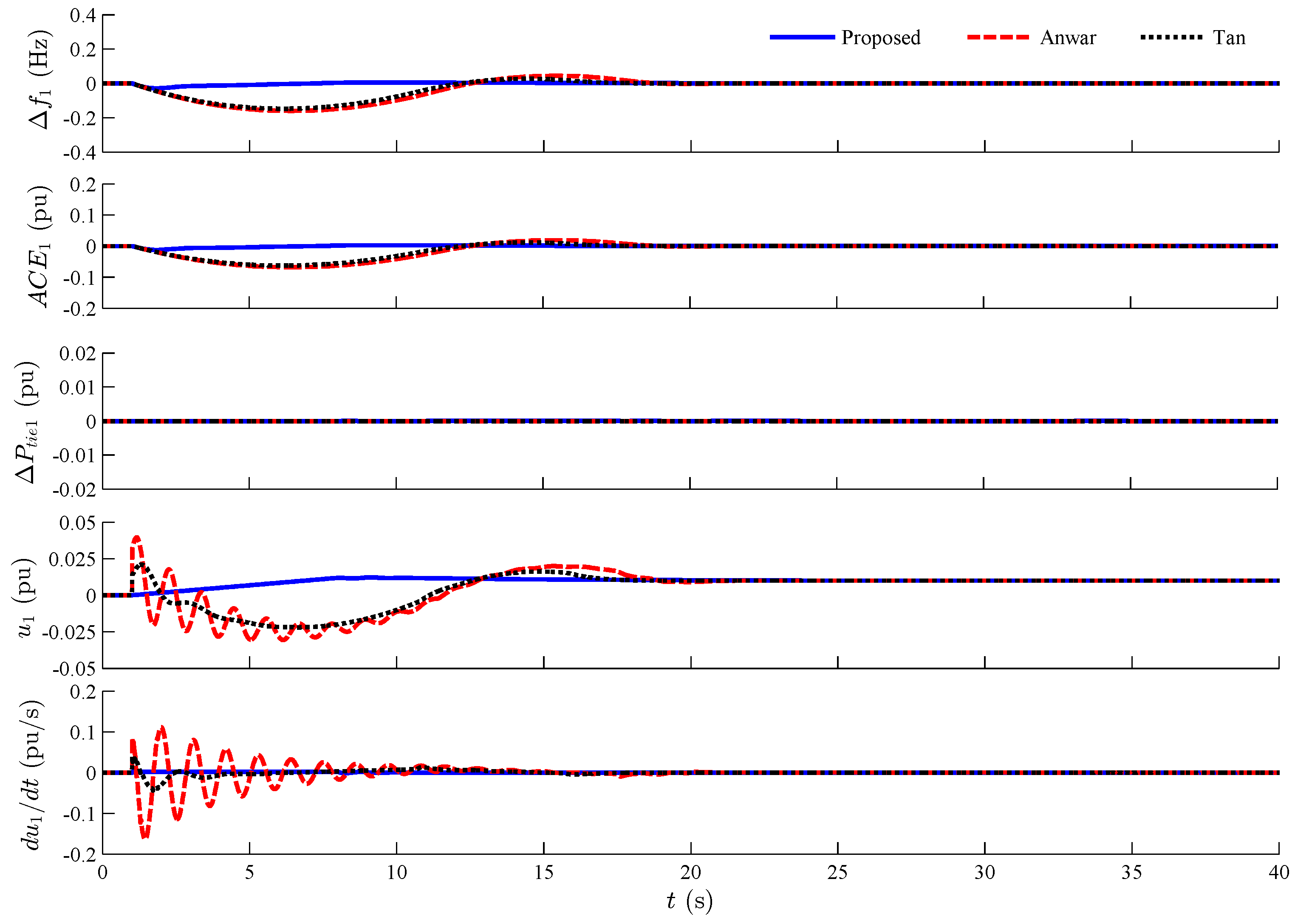
4.1. Scenario 1: Simulations on Single-Area System

In Scenario 1, we set the same load disturbances in the two areas of the system shown in Figure 4. By this way, each area can be treated as a single-area system, since the two areas have the same structure and parameters.
Towards the LFC model of the test system, by the proposed method, we design the anti-windup LFC consisting of a robust H dynamic controller, a linear filter, a magnitude and rate saturation loop, and an AWC as follows:
The robust H dynamic controller:
C ¯ : x ˙ c ¯ = A c ¯ x c ¯ + B c ¯ u c ¯ y c ¯ = C c ¯ x c ¯ + D c ¯ u c ¯
where:
A c ¯ = 9 . 94374 2 . 32119 0 . 620889 4 . 096447 312 . 625 21 . 43163 15 . 2773 0 . 43206 12 . 18535 1229 . 041 117 . 987 167 . 214 881 . 295 93 . 2623 113 . 066 2211 . 94 3412 . 12 1198 . 68 15702 . 6 189 . 4382 759871 . 3 734389 395045 84813 . 64 157822
B c ¯ = 146 . 091 153 . 625 1 . 605 894 . 647 414 . 317 405 . 444 8964 . 850 4553 . 067 240549 . 496 641800 . 483 1031816 . 318 31109 . 807 54307506 . 731 30731255 . 138 1104996 . 282
C c ¯ = 0 . 027 0 . 024 0 . 006 0 . 041 3 . 200
D c ¯ = 1 . 134 1 . 560 0 . 006
The linear filter (approximate differentiator):
s / ( 1 + τ s ) = s / ( 1 + 0 . 01 s )
The magnitude and rate bounds of the control input:
[ m ̲ , m ¯ ] = [ 0 . 1 , 0 . 1 ] , [ r ̲ , r ¯ ] = [ 0 . 0017 , 0 . 0017 ]
The AWC:
x ˙ aw φ ˙ aw = A B u 0 0 + 0 I K aw x aw φ aw
where K aw = [ 0 . 908 3 . 929 1 . 367 3 . 777 3 . 162 6 . 646 ] .
Based on the designed anti-windup LFC Equations (11)–(14), we make two tests: one is for step load decrease Δ P L 1 = Δ P L 2 = 0 . 015 ( pu ) , the other is for step load increase Δ P L 1 = Δ P L 2 = 0 . 01 ( pu ) . The system responses to the load decrease and increase are shown in Figure 5 and Figure 6, respectively. Considering that Area 1 and 2 have the same responses, we only illustrate the simulation results of Area 1. The concerned variables, such as frequency deviation Δ f , ACE, tie-line power deviation Δ P tie , control input u, and rate of control input d u / d t , are shown in Figure 5 and Figure 6.
From the results of both of the above tests, it is shown that, compared with the controllers presented by Tan and by Anwar, the proposed controller generates smaller overshoot and takes shorter settling time to force the frequency deviation and ACE to zeros. Furthermore, seeing from the control input curves, one can find that the control signal of the proposed controller in this paper meets the prescribed magnitude and rate constraint, while the control signals of Tan’s and Anwar’s controllers exceed the rate constraint. Here, it should be noted that Δ P tie is always equal to zero since there is no tie-line power deviation between the two symmetrical areas.

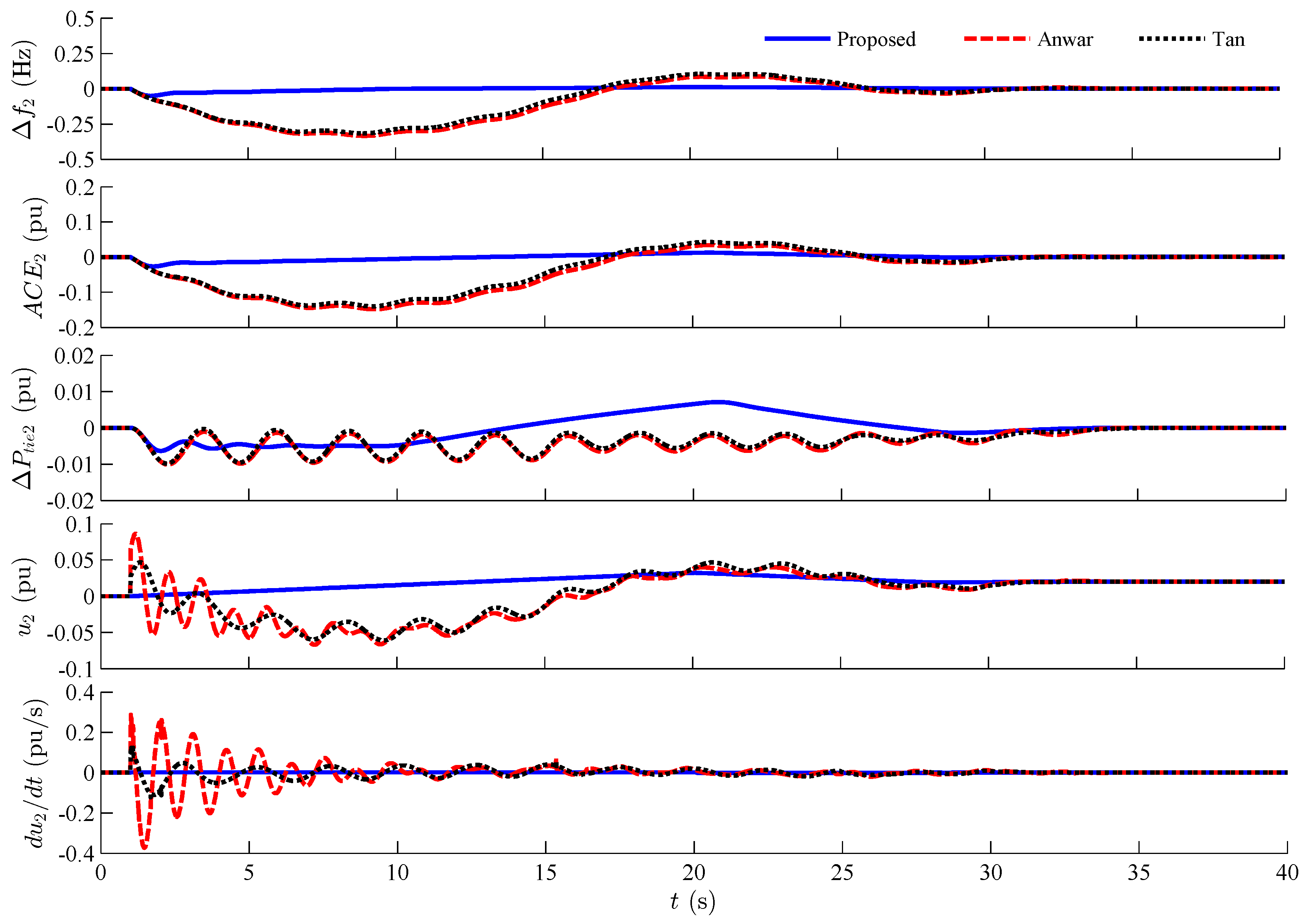
4.2. Scenario 2: Simulations on a Two-Area System

The anti-windup LFC in Scenario 2 is the same as the controller Equations (11)–(14) in Scenario 1, since the parameters of the area model are identical in both systems. In this scenario, different load disturbances are set for two tests as: Δ P L 1 = 0 . 01 ( pu ) and Δ P L 2 = 0 . 02 ( pu ) for Test 1; Δ P L 1 = 0 . 02 ( pu ) and Δ P L 2 = 0 . 01 ( pu ) for Test 2. The simulations are performed on the two-area system directly, and the results are shown in Figure 7, Figure 8, Figure 9 and Figure 10.
From the results in Figure 7, Figure 8, Figure 9 and Figure 10, it is observed that all the three controllers can drive the system frequency deviation, the ACE and the tie-line power deviation to zero, but the proposed anti-windup controller obtains more favorable performances than the other two controllers at aspect of overshoot and settling time. In addition, unlike Tan’s method and Anwar’s method, the proposed method avoids the undesired oscillation. Seeing the control input u, we also find that the proposed anti-windup controller can match the magnitude and rate constraint. Therefore, the system can operate in the linear region, and thus the nonlinear GRC is tackled.
By comparing the results in Scenario 1 and Scenario 2, it can be observed that the control performances of Scenario 1 are better than that of Scenario 2. The reason is that, in Scenario 1, the controller only needs to attenuate the local load disturbance, but, in Scenario 2, both the load disturbance in local area and the tie-line power disturbance from the neighboring area are needed to be restrained.

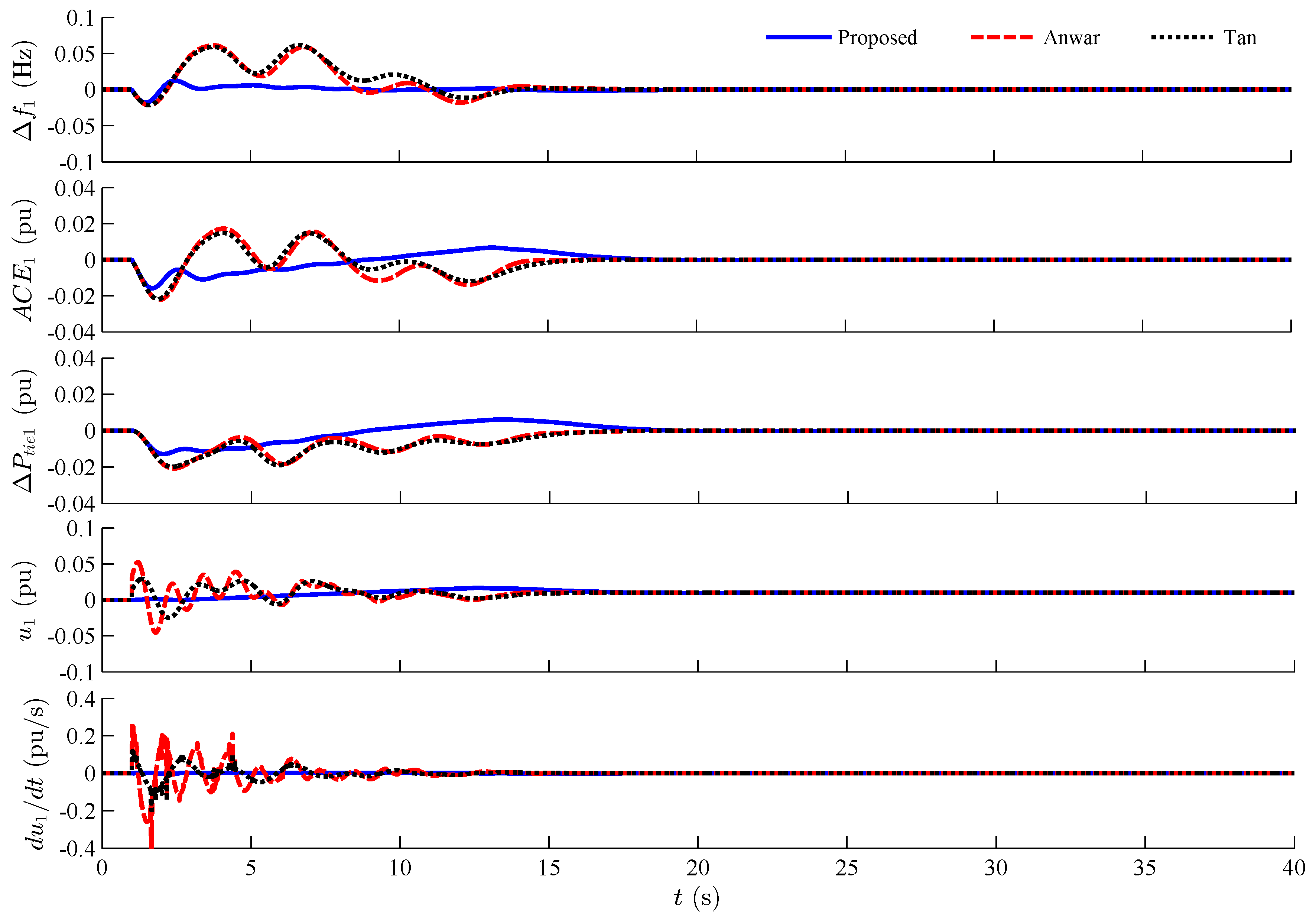
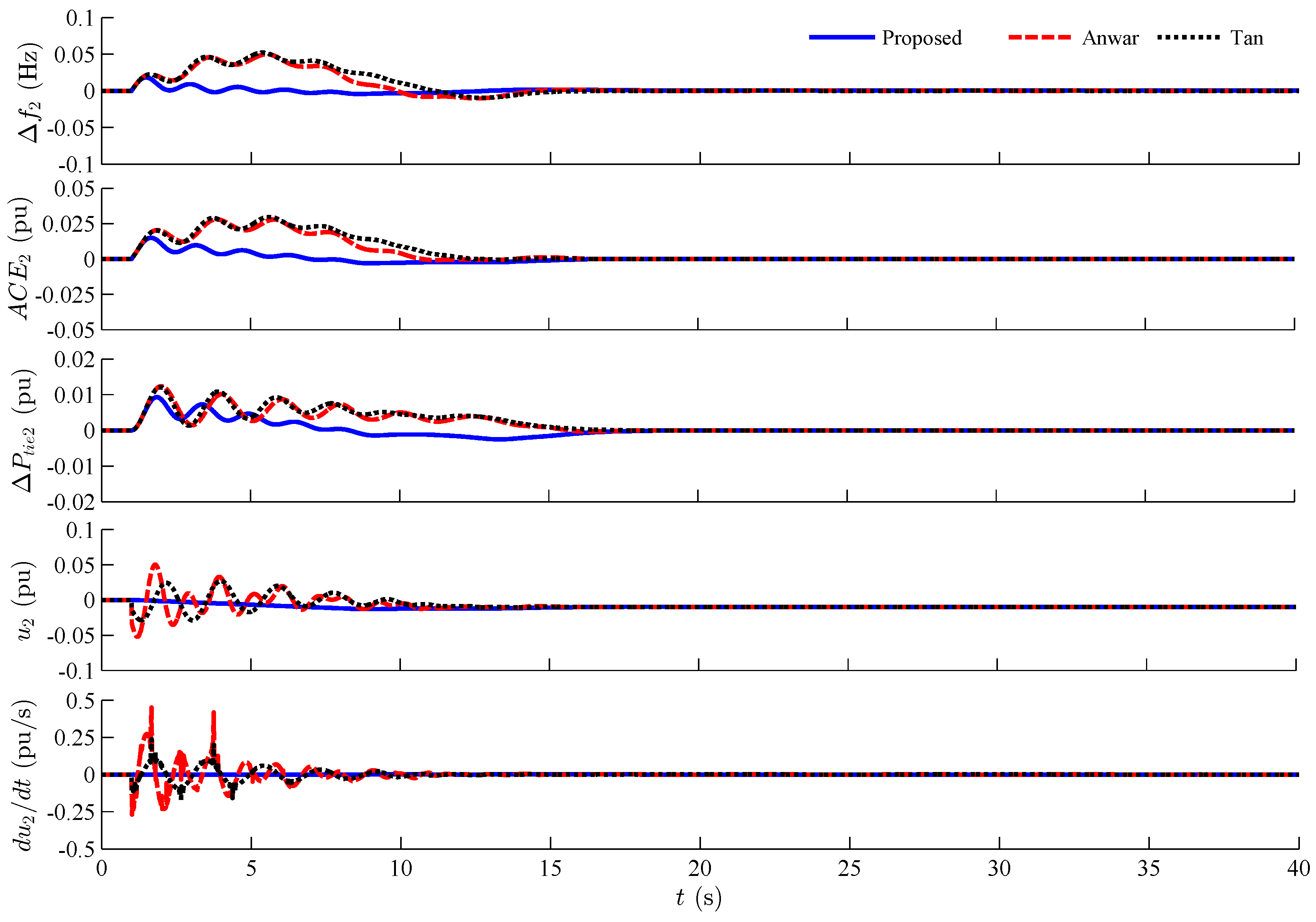
4.3. Scenario 3: Simulations on Three-Area Systems

In Scenario 3, the two-area system shown in Figure 4 is changed into two three-area interconnected systems. One is a chain-type system shown in Figure 11, the other is a delta-type system shown in Figure 12. For simplicity, we make the parameters of each area in the three-area systems be the same to those in the two-area system. In addition, the tie-line synchronizing coefficients are selected as: for the chain-type system, T 12 = T 21 = T 23 = T 32 = 0 . 545 ( pu / Hz ) , γ 1 = T 12 = 0 . 545 ( pu / Hz ) , γ 2 = T 21 + T 23 = 1 . 09 ( pu / Hz ) , γ 3 = T 32 = 0 . 545 ( pu / Hz ) ; for the delta-type system, T 12 = T 21 = T 23 = T 32 = T 13 = T 31 = 0 . 545 ( pu / Hz ) , γ 1 = T 12 + T 13 = 1 . 09 ( pu / Hz ) , γ 2 = T 21 + T 23 = 1 . 09 ( pu / Hz ) , γ 3 = T 31 + T 32 = 1 . 09 ( pu / Hz ) .
For Areas 1 and 3 of the chain-type system, their anti-windup LFC are the same as the one in Scenario 1, namely Equations (11)–(14), since these area models have identical parameters in Equation (3). For Area 2, however, the anti-windup LFC needs to be redesigned, because the parameter γ 2 in the matrix A in Equation (3) is not equal to γ 1 . Based on the given parameters, a robust H dynamic controller and an AWC are designed for Area 2 as follows:
The robust H dynamic controller:
C ¯ : x ˙ c ¯ = A c ¯ x c ¯ + B c ¯ u c ¯ y c ¯ = C c ¯ x c ¯ + D c ¯ u c ¯
where:
A c ¯ = 9 . 357 2 . 267 2 . 343 5 . 018 535 . 792 18 . 070 16 . 938 0 . 246 5 . 616 1531 . 194 149 . 396 236 . 362 1083 . 630 183 . 093 381 . 424 233 . 018 2806 . 868 1859 . 898 7169 . 953 314 . 377 1014222 . 355 978906 . 090 830564 . 259 430071 . 155 251967 . 406
B c ¯ = 154 . 484 127 . 097 2 . 559 902 . 163 213 . 902 704 . 383 2720 . 065 11933 . 119 116445 . 141 222855 . 373 438613 . 914 30897 . 537 68477106 . 358 11506520 . 276 1200741 . 256
C c ¯ = 0 . 040 0 . 028 0 . 030 0 . 062 6 . 652
D c ¯ = 1 . 532 1 . 569 0 . 002
The AWC:
x ˙ aw φ ˙ aw = A B u 0 0 + 0 I K aw x aw φ aw
where K aw = [ 0 . 908 3 . 929 1 . 367 3 . 777 3 . 162 6 . 646 ] .
Combining the above robust controller and AWC with the bounds of the control input and the linear filter presented in Scenario 1, we obtain the anti-windup LFC of Area 2, namely, Equations (12), (13), (15) and (16).
In summary, for the three-area chain-type system, the anti-windup LFCs are described as: Equations (11)–(14) for Area 1 and 3; Equations (12), (13), (15) and (16) for Area 2. For the three-area delta-type system, the anti-windup LFCs are expressed as Equations (12), (13), (15) and (16) for Area 1, 2, and 3, since the three areas in the delta-type system have the same parameters as Area 2 in the chain-type system.
In Scenario 3, the load disturbances are set as: in the chain-type system, P L 1 = 0 . 01 ( pu ) in Area 1, P L 2 = 0 . 01 ( pu ) in Area 2, and P L 3 = 0 . 01 ( pu ) in Area 3; in the delta-type system, P L 1 = 0 . 02 ( pu ) in Area 1, P L 2 = 0 . 01 ( pu ) in Area 2, and P L 3 = 0 . 01 ( pu ) in Area 3.
The results are shown in Figure 13, Figure 14 and Figure 15 for the chain-type system and Figure 16, Figure 17 and Figure 18 for the delta-type system. The simulations reveal that the proposed method can restrain the load disturbances, regulate the frequency of each area, and restore the tie-line power to its scheduled value. In other words, the proposed method can realize the LFC objectives of multi-area interconnected power system. Compared with Tan’s method and Anwar’s method, the method in this paper obtains better performances in overshoot and settling time. The magnitude and rate of the input signals are especially controlled in the predetermined ranges by the proposed anti-windup controller, which helps to reduce the wear and tear of generators and improve the stability of the closed-loop system.

5. Conclusions

Towards the GRC problem in the LFC, this paper proposes an anti-windup controller design method. In the anti-windup LFC, the H dynamic controller is designed to guarantee robust performance against load disturbances and tie-line power disturbances, and the AWC is used to restrict the magnitude and rate of the control input so that the system can operate in the linear region to overcome the GRC. The simulation results show that the proposed anti-windup LFC design method effectively improves the performances against disturbances and GRC. Further work will focus on the coordination method of different LFCs to improve the overall performances of the multi-area interconnected power system.

Acknowledgments

This project is supported by the National Natural Science Foundation of China (Nos. 51507085 and 61533010) and the Scientific Fund of Nanjing University of Posts and Telecommunications (NUPTSF Grants No.NY214202 and No.XJKY14018).

Author Contributions

Chongxin Huang and Dong Yue designed the control strategy and wrote the manuscript; Xiangpeng Xie analyzed the results; Jun Xie checked the whole manuscript.

Conflicts of Interest

The authors declare no conflict of interest.

References

  1. Rerkpreedapong, D.; Hasanovic, A.; Feliachi, A. Robust load frequency control using genetic algorithms and linear matrix inequalities. IEEE Trans. Power Syst. 2003, 18, 855–861. [Google Scholar] [CrossRef]
  2. Shayeghi, H.; Shayanfar, H.A.; Jalili, A. Load frequency control strategies: A state-of-the-art survey for the researcher. Energy Convers. Manag. 2009, 50, 344–353. [Google Scholar] [CrossRef]
  3. Khodabakhshian, A.; Edrisi, M. A new robust PID load frequency controller. Control Eng. Pract. 2008, 16, 1069–1080. [Google Scholar] [CrossRef]
  4. Tan, W. Unified tuning of PID load frequency controller for power systems via IMC. IEEE Trans. Power Syst. 2010, 25, 341–350. [Google Scholar] [CrossRef]
  5. Ghoshal, S.P. Application of GA/GA-SA based fuzzy automatic generation control of a multi-area thermal generating system. Electr. Power Syst. Res. 2004, 70, 115–127. [Google Scholar] [CrossRef]
  6. Cam, E.; Kocaarslan, I. Load frequency control in two area power systems using fuzzy logic controller. Energy Convers. Manag. 2005, 46, 233–243. [Google Scholar] [CrossRef]
  7. Sabahi, K.; Teshnehlab, M.; Shoorhedeli, M.A. Recurrent fuzzy neural network by using feedback error learning approaches for LFC in interconnected power system. Energy Convers. Manag. 2009, 50, 938–946. [Google Scholar] [CrossRef]
  8. Bevrani, H.; Daneshmand, P.R.; Babahajyani, P.; Mitani, Y.; Hiyama, T. Intelligent LFC concerning high penetration of wind power: Synthesis and real-time application. IEEE Trans.Sustain.Energy 2014, 5, 655–662. [Google Scholar] [CrossRef]
  9. Sahu, R.K.; Panda, S.; Pradhan, P.C. Design and analysis of hybrid firefly algorithm-pattern search based fuzzy PID controller for LFC of multi area power systems. Int. J. Electr. Power Energy Syst. 2015, 69, 200–212. [Google Scholar] [CrossRef]
  10. Al-Hamouz, Z.M.; Al-Duwaish, H.N. A new load frequency variable structure controller using genetic algorithms. Electr. Power Syst. Res. 2000, 55, 1–6. [Google Scholar] [CrossRef]
  11. Vrdoljak, K.; Perić, N.; Petrović, I. Sliding mode based load-frequency control in power systems. Electr. Power Syst. Res. 2010, 80, 514–527. [Google Scholar] [CrossRef]
  12. Al-Hamouz, Z.; Al-Duwaish, H.; Al-Musabi, N. Optimal design of a sliding mode AGC controller: Application to a nonlinear interconnected model. Electr. Power Syst. Res. 2011, 81, 1403–1409. [Google Scholar] [CrossRef]
  13. Aldeen, M.; Trinh, H. Load-frequency control of interconnected power systems via constrained feedback control schemes. Comput. Electr. Eng. 1994, 20, 71–88. [Google Scholar] [CrossRef]
  14. Alrifai, M.T.; Hassan, M.F.; Zribi, M. Decentralized load frequency controller for a multi-area interconnected power system. Int. J. Electr. Power Energy Syst. 2011, 33, 198–209. [Google Scholar] [CrossRef]
  15. Trinh, H.; Fernando, T.; Iu, H.H.C.; Wong, K.P. Quasi-decentralized functional observers for the LFC of interconnected power systems. IEEE Trans. Power Syst. 2013, 28, 3513–3514. [Google Scholar] [CrossRef]
  16. Pham, T.N.; Trinh, H.; Hien, L.V. Load frequency control of power systems with electric vehicles and diverse transmission links using distributed functional observers. IEEE Trans. Smart Grid 2016, 7, 238–252. [Google Scholar] [CrossRef]
  17. Rahmani, M.; Sadati, N. Hierarchical optimal robust load-frequency control for power systems. IET Gener. Transm. Distrib. 2012, 6, 303–312. [Google Scholar] [CrossRef]
  18. Vachirasricirikul, S.; Ngamroo, I. Robust LFC in a smart grid with wind power penetration by coordinated V2G control and frequency controller. IEEE Trans. Smart Grid 2014, 5, 371–380. [Google Scholar] [CrossRef]
  19. Dong, L.L.; Zhang, Y.; Gao, Z.Q. A robust decentralized load frequency controller for interconnected power systems. ISA Trans. 2012, 51, 410–419. [Google Scholar] [CrossRef] [PubMed]
  20. Jiang, L.; Yao, W.; Wu, Q.H.; Wen, J.Y.; Cheng, S.J. Delay-dependent stability for load frequency control with constant and time-varying delays. IEEE Trans. Power Syst. 2012, 27, 932–941. [Google Scholar] [CrossRef]
  21. Dey, R.; Ghosh, S.; Ray, G.; Rakshit, A. H load frequency control of interconnected power systems with communication delays. Int. J. Electr. Power Energy Syst. 2012, 42, 672–684. [Google Scholar] [CrossRef]
  22. Zhang, C.K.; Jiang, L.; Wu, Q.H.; He, Y.; Wu, M. Delay-dependent robust load frequency control for time delay power systems. IEEE Trans. Power Syst. 2013, 28, 2192–2201. [Google Scholar] [CrossRef]
  23. Atić, N.; Rerkpreedapong, D.; Hasanović, A.; Feliachi, A. NERC compliant decentralized load frequency control design using model predictive control. In Proceedings of the IEEE on Power Engineering Society General Meeting, Toronto, ON, Canada, 13–17 July 2003.
  24. Franze, G.; Tedesco, F. Constrained load/frequency control problems in networked multi-area power systems. J. Frankl. Inst. 2011, 348, 832–852. [Google Scholar] [CrossRef]
  25. Tedesco, F.; Casavola, A. Fault-tolerant distributed load/frequency supervisory strategies for networked multi-area microgrids. Int. J. Robust Nonlinear Control 2014, 24, 1380–1402. [Google Scholar] [CrossRef]
  26. Moon, Y.H.; Ryu, H.S.; Lee, J.G.; Song, K.B.; Shin, M.C. Extended integral control for load frequency control with the consideration of generation-rate constraints. Int. J. Electr. Power Energy Syst. 2002, 24, 263–269. [Google Scholar] [CrossRef]
  27. Velusami, S.; Chidambaram, I.A. Decentralized biased dual mode controllers for load frequency control of interconnected power systems considering GDB and GRC non-linearities. Energy Convers. Manag. 2007, 48, 1691–1702. [Google Scholar] [CrossRef]
  28. Sudha, K.R.; Santhi, R.V. Robust decentralized load frequency control of interconnected power system with generation rate constraint using Type-2 fuzzy approach. Int. J. Electr. Power Energy Syst. 2011, 33, 699–707. [Google Scholar] [CrossRef]
  29. Tan, W. Tuning of PID load frequency controller for power systems. Energy Convers. Manag. 2009, 50, 1465–1472. [Google Scholar] [CrossRef]
  30. Anwar, M.N.; Pan, S. A new PID load frequency controller design method in frequency domain through direct synthesis approach. Int. J. Electr. Power Energy Syst. 2015, 67, 560–569. [Google Scholar] [CrossRef]
  31. Forni, F.; Galeani, S.; Zaccarian, L. Model recovery anti-windup for plants with rate and magnitude saturation. In Proceedings of the European Control Conference, Budapest, Hungary, 23–26 August 2009; pp. 324–329.
  32. Forni, F.; Galeani, S.; Zaccarian, L. An almost anti-windup scheme for plants with magnitude, rate and curvature saturation. In Proceedings of the American Control Conference, Baltimore, MD, USA, 30 June–2 July 2010; pp. 6769–6774.
  33. Chilali, M.; Gahinet, P. H design with pole placement constraints: An LMI approach. IEEE Trans. Autom. Control 1996, 41, 358–367. [Google Scholar] [CrossRef]
  34. Scherer, C.; Gahinet, P.; Chilali, M. Multiobjective output-feedback control via LMI optimization. IEEE Trans. Autom. Control 1997, 42, 896–911. [Google Scholar] [CrossRef]
  35. Gahinet, P.M.; Nemirovskii, A.; Laub, A.J.; Chilali, M. The LMI control toolbox. In Proceedings of the 33rd IEEE Conference on Decision and Control, Lake Buena Vista, FL, USA, 14–16 December 1994; pp. 2038–2038.
  36. Forni, F.; Galeani, S.; Zaccarian, L. Model recovery anti-windup for continuous-time rate and magnitude saturated linear plants. Automatica 2012, 48, 1502–1513. [Google Scholar] [CrossRef]
Figure 1. Load frequency control (LFC) diagram of Area i. ACE: area control error; GRC: generation rate constraint.
Energies 09 00330 g001
Figure 2. Modified LFC diagram of Area i.
Energies 09 00330 g002
Figure 3. Structure of an anti-windup control scheme. AWC: anti-windup compensator.
Energies 09 00330 g003
Figure 4. Diagram of a two-area interconnected power system.
Energies 09 00330 g004
Figure 5. Results for load decrease in a single-area system.
Energies 09 00330 g005
Figure 6. Results for load increase in a single-area system.
Energies 09 00330 g006
Figure 7. Results of Area 1 in a two-area system for Test 1.
Energies 09 00330 g007
Figure 8. Results of Area 2 in a two-area system for Test 1.
Energies 09 00330 g008
Figure 9. Results of Area 1 in a two-area system for Test 2.
Energies 09 00330 g009
Figure 10. Results of Area 2 in a two-area system for Test 2.
Energies 09 00330 g010
Figure 11. Diagram of a three-area chain-type interconnected power system.
Energies 09 00330 g011
Figure 12. Diagram of a three-area delta-type interconnected power system.
Energies 09 00330 g012
Figure 13. Results of Area 1 in a three-area chain-type system.
Energies 09 00330 g013
Figure 14. Results of Area 2 in a three-area chain-type system.
Energies 09 00330 g014
Figure 15. Results of Area 3 in a three-area chain-type system.
Energies 09 00330 g015
Figure 16. Results of Area 1 in a three-area delta-type system.
Energies 09 00330 g016
Figure 17. Results of Area 2 in a three-area delta-type system.
Energies 09 00330 g017
Figure 18. Results of Area 3 in a three-area delta-type system.
Energies 09 00330 g018

