Dynamic Equivalent Modeling for Small and Medium Hydropower Generator Group Based on Measurements

Abstract

At present, the common practice in the power system of China is to represent the small and medium hydropower generator group as a negative load. This paper presents a method to build a dynamic equivalent model of the hydropower generator group using a 3rd order generator model and a static characteristic load model. Based on phasor measurements in the tie line which connects to the modeled hydropower generator group, the dynamic multi-swarm particle swarm optimizer (DMS-PSO) algorithm is used to obtain parameters of the equivalent model. The proposed method is verified in the small and medium hydropower generator group of Sichuan power grid with both simulation and actual data. The results show that the dynamic responses and the transient stability are consistent before and after the equivalence. The proposed method can be used for modeling a group of small and medium hydropower generators whose structures and parameters are unknown.

1. Introduction

There are a large number of small and medium hydropower generators in abundant water resources areas because they are flexible, convenient and environmentally-friendly energy sources. If the region contains a lot of small and medium hydropower stations, the dynamic performance of the power system must be affected by the hydropower generator group. It is difficult to establish a detailed model because the parameters of each generating unit can barely be obtained if there is a small and medium hydropower generator group in the power system. The power flow calculation may not be converged and the dimension is too large for dynamic analysis, even if the typical parameters are used. At present, the common practice in the power system of China is to represent the small and medium hydropower generator group as a negative load, but the simulation results are not accurate. Dynamic equivalence is an accurate way to represent the characteristics of the equivalent system [1].

At present, the dynamic equivalence methods can be divided into three categories. The first one is the coherency-based equivalent method. In [2,3,4], the hydropower generator group is equivalent to a 3rd order generator and a load with a weighted average method, while a 4th order generator and a load are used as the equivalent model for the hydropower generator group in [5]. However, there are significant limitations when using the traditional coherency-based equivalent method to construct the equivalent model because the structures and parameters of the hydropower generator group must be known [6,7]. The second one is modal-based equivalent method. However, it is not appropriate to transient stability analysis because nonlinear models are linearized and state equations are used as the equivalent model [8,9,10,11]. The third one is estimation-based equivalent method, which functions only by making use of measurements. The estimation equivalent method is first proposed in paper [12]. Scholars have undertaken further study in the estimation-based equivalent method in two branches. A 16-machine test system is equivalent to using artificial neural networks in [13,14,15]. A 2nd order transfer function is proposed to equal the distributed network cell based on Prony analysis and nonlinear least square optimization method [16]. However, there is no physical meaning for these equivalent models. The other branch also has some disadvantages. A CEPRI 8-machine test system is equivalent to a 3rd order generator and a static characteristic load model with linearized approach during the process of calculating the equivalent model parameters so that the results are not accurate enough as a nonlinear method [17]. The eight generators are equivalent to a 3rd order generator based on PSASP (Power System Analysis Software Package) transient stability module and particle swarm optimizer (PSO) [18], but there is not much practical significance because the internal system model must be combined. Moreover, there is little research on dynamic equivalence for the small and medium hydropower generator group based on the estimation-based equivalent method. Therefore, it is significant to research the estimation-based equivalent method based on phasor measurements while the structures and parameters of the hydropower generator group are unknown.

In this paper, a measurement-based method for system dynamic equivalence is proposed to construct the dynamic equivalent model for a small and medium hydropower generator group whose structures and parameters are unknown. The proposed equivalent model is a parallel dynamic equivalent model composed of a 3rd order electromechanical transient generator model with damping and a static characteristic load model considering voltage. Based on the tie line phasor measurements, parameters of the equivalent model are obtained by combining nonlinear 4th order Runge-Kutta method and dynamic multi-swarm particle swarm optimizer (DMS-PSO) algorithm. The proposed method is verified in the small and medium hydropower generator group of Sichuan power grid with both simulation and actual data.

The rest of this paper is organized as follows. The equivalent model for the small and medium hydropower generator group is introduced in Section 2. In Section 3, methodology of the proposed equivalence is presented. The proposed equivalent model is validated by the case study in the Sichuan power grid with both simulation and actual data being presented in Section 4. Section 5 concludes this paper.

2. Equivalent Model for the Hydropower Generator Group

The small and medium hydropower generator group is always connected to the internal system through a tie line, and the electrical distance of each hydropower generator in the equivalent area is relatively close. Therefore, the hydropower generator group can be considered coherent when disturbances occur within the internal system [19]. Based on the above characteristics, the dynamic equivalent model is shown in Figure 1, which is in the form of a single generator and a parallel single load.

2.1. Equivalent Generator Model

The 2nd order generator model for system equivalence cannot accurately represent the dynamic behaviors of the original system since the 2nd order generator model does not consider the field winding and damping winding. The performances of different dynamic equivalent models are analyzed in [20], and the results show that the 3rd order generator model is good enough for accurate equivalence since the optimization time greatly increased with the 5th order generator model without improving accuracy significantly. In this paper, the 3rd order generator model is used by considering field windings and damping windings, and the proportional feedback model is used in an excitation system while the constant torque model is used in the speed control system. The equations of the generator model are:

$$\{\begin{array}{l}{T}_j\frac{\mathrm{d}\mathsf{\omega }}{\mathrm{d}t}=P_{\mathrm{m}}-\frac{E^{\prime }V}{{x^{\prime }}_{\mathrm{d}}}\sin \mathsf{\delta }-D\frac{\mathrm{d}\mathsf{\delta }}{\mathrm{d}t}\hfill \\ \frac{\mathrm{d}\mathsf{\delta }}{\mathrm{d}t}=\left(\mathsf{\omega }-{\mathsf{\omega }}_{\mathrm{f}}\right){\mathsf{\omega }}_0,{\mathsf{\omega }}_0=2\mathsf{\pi }f\hfill \\ T_{\mathrm{d}0}^{\prime }\frac{\mathrm{d}{E}^{\prime }}{\mathrm{d}t}=E_{\mathrm{f}0}-K_{\mathrm{V}}(V-V_0)-\frac{x_{\mathrm{d}}}{{x^{\prime }}_{\mathrm{d}}}{E}^{\prime }+(\frac{x_{\mathrm{d}}}{{x^{\prime }}_{\mathrm{d}}}-1)V\cos \mathsf{\delta }\hfill \end{array}$$

(1)

where T_j is the inertia time constant; P_m is the mechanical power; E^′ is the electromotive force after x^′_d and instead of q-axis transient electromotive force; V is the generator voltage; x^′_d is the d-axis transient reactance and the value is equal to q-axis synchronous reactance; δ is the power angle; D is the damping coefficient; t is time; ω is the rotor speed of generator; ω_f is the rotor speed of reference; T^′_d0 is the d-axis transient open circuit time constant; E_f0 is the initial excitation voltage; K_v is the feedback coefficient of excitation voltage; V₀ is the initial generator voltage; x_d is the d-axis synchronous reactance.

2.2. Equivalent Load Model

Due to less influence to the system dynamic characteristics by the equivalent load, the static load model considering voltage is taken as the equivalent load model. The identifiability of a 3rd order generator and a static load is proved by the theory in [19]. The load model equations are:

$$\{\begin{array}{l}{P}_{\mathrm{s}}=P_{\text{s0}}{(\frac{V}{V_0})}^{\text{Np}}\\ Q_{\mathrm{s}}=Q_{\text{s0}}{(\frac{V}{V_0})}^{\text{Nq}}\end{array}$$

(2)

where P_s is the load active power; P_s0 is the initial load active power; N_p is the index of voltage characteristics on active power; Q_s is the load reactive power; Q_s0 is the initial load reactive power; N_q is the index of voltage characteristics on reactive power.

From the foregoing analysis, the power equations in tie line can be described as follows:

$$\{\begin{array}{l}{P}_{\mathrm{l}}=P_{\mathrm{e}}-P_{\mathrm{s}}\\ Q_{\mathrm{l}}=Q_{\mathrm{e}}-Q_{\mathrm{s}}\end{array}$$

(3)

where P_l is the active power in tie line; Q_l is the reactive power in tie line; P_e is the generator active power; Q_e is the generator reactive power.

3. Methodology of the Proposed Equivalence

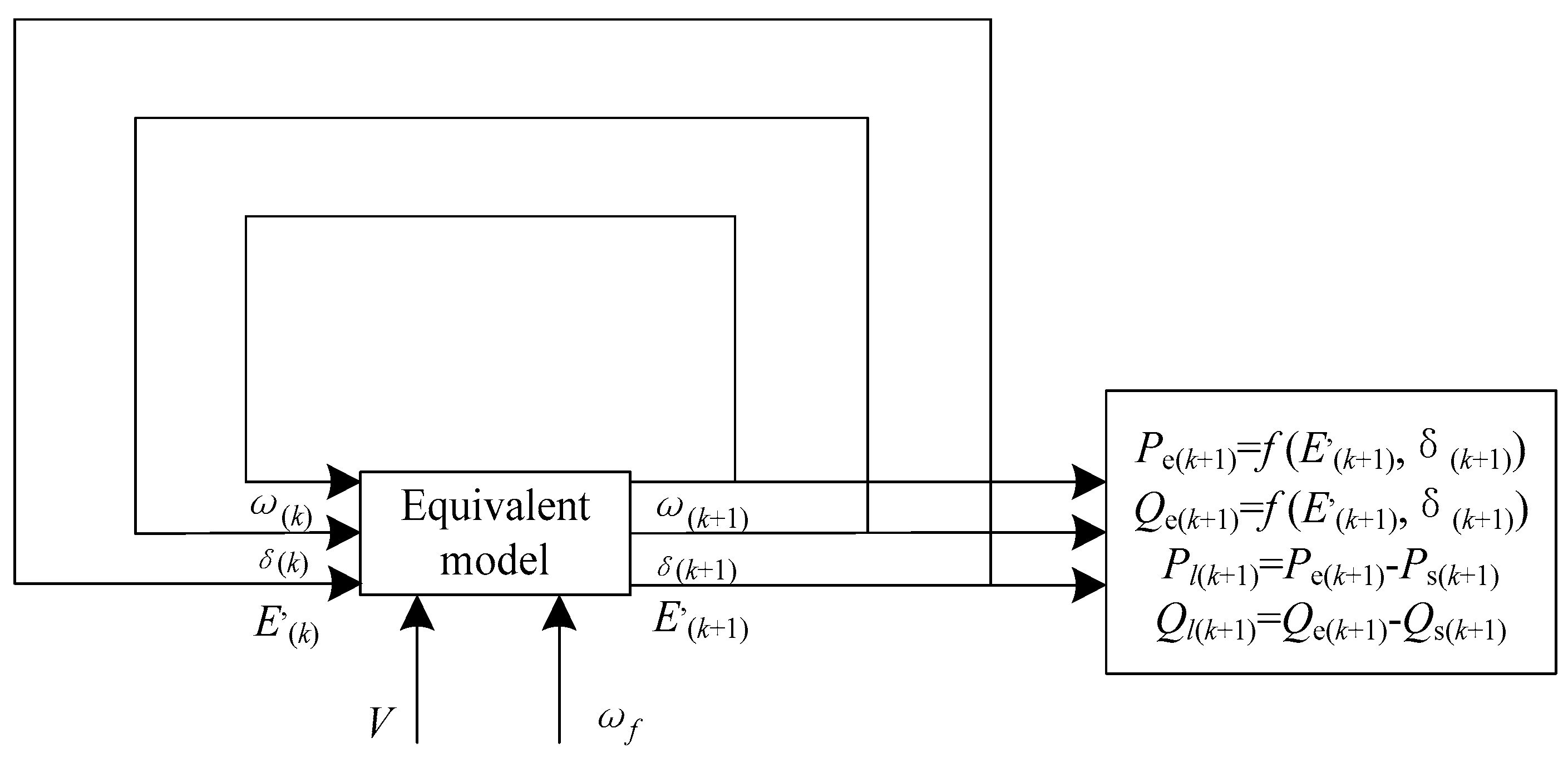
3.1. Frame of the Equivalence Method

Synchronized phasor measurement technology has been widely used in the power system dynamic monitoring [21,22,23]. Equivalent model parameters are obtained by making use of dynamic information in the tie line during the disturbance based on the parameter estimation. In this paper, the measurements of voltage, frequency, active power and reactive power in the tie line are extracted as inputs and then the equivalent model parameters are identified, which is α = [T_j, x_d, x^’_d, T^’_d0, K_v, D, P_s0, Q_s0, N_p, N_q]. The overall framework is shown in Figure 2.

The processes are as follows: firstly, initialize a suspicious parameter α; secondly, take the voltage and frequency responses in the tie line as inputs; thirdly, solve the equations of equivalent model and get active and reactive power; then compare measured and calculated values of the active and reactive power and the error e is generated; finally compare the error with the set threshold, namely if the error is greater, update parameter α by the optimization algorithm and repeat the process; otherwise, output α as the equivalent model parameters.

The electrical power outputs are calculated with the following equations:

$$\{\begin{array}{l}{P}_{\mathrm{e}(k)}=\frac{{E^{\prime }}_{(k)}{V}_{(k)}}{x_{\mathrm{d}}^{\prime }}\sin ({\mathsf{\delta }}_{(k)})\\ Q_{\mathrm{e}(k)}=\frac{{E^{\prime }}_{(k)}{V}_{(k)}\cos ({\mathsf{\delta }}_{(k)})-{V^2}_{(k)}}{x_{\mathrm{d}}^{\prime }}\end{array}$$

(4)

The error is calculated with the Euclidean distance formula:

$$e={\displaystyle \sum _{k=1}^N\sqrt{{(\frac{P_{\mathrm{l}(k)}-P_{\mathrm{l}(k)}^{\prime }}{P_{\mathrm{l}(1)}})}^2+{(\frac{Q_{\mathrm{l}(k)}-Q_{\mathrm{l}(k)}^{\prime }}{Q_{\mathrm{l}(1)}})}^2}}$$

(5)

where N is the total number of sampling sites; P_l is the measured value of active power; P^′_l is the calculated value of active power; Q_l is the measured value of reactive power; Q^′_l is the calculated value of reactive power.

In order to obtain the electrical power outputs, the δ and E^′ from different times have to be calculated. The two most classic numerical methods are the improved Euler method and Runge-Kutta method [24]. The 4th order Runge-Kutta method is used widely when solving ordinary differential equations because of its briefness and accuracy [25,26,27]. In this paper, the 4th order Runge-Kutta method is used to solve generator dynamic equations and the state variables of time k + 1 moment such as ω, δ, E^′ can be calculated by time k moment. The initial value of state variables can be determined by the steady-state phasor diagram. The power outputs in the tie line are obtained with the certain equivalent model parameters based on Equations (1)–(4). The frame is shown in Figure 3.

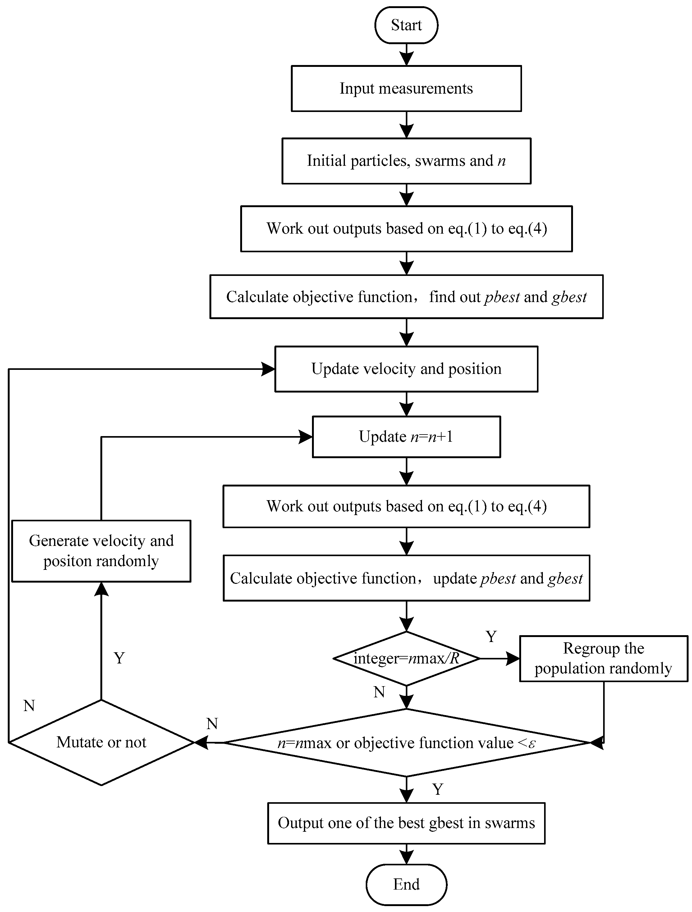
3.2. Dynamic Multi-Swarm Particle Swarm Optimizer Algorithm

The PSO algorithm is widely used in the optimization of power system because of its good global convergence, easy operation, high efficiency and few parameter settings [28,29,30]. In this paper, equivalent model parameters are identified by the DMS-PSO algorithm [31].

The optimal solution is found by initializing a group of random particles, iterating them repeatedly with the basic method of PSO. In each iteration process, the particles are updated by tracking two “extremes”: one is the optimal solution found by an individual (personal best, that is pbest), and the other is the optimal solution found by the entire group (group best, that is gbest). Each particle updates its velocity and position respectively according to the following equations.

$$\{\begin{array}{l}{v}_{n+1}=w{v}_n+c_1\times rand\times (pbes{t}_n-x_n)+c_2\times rand\times (gbes{t}_n-x_n)\hfill \\ x_{n+1}=x_n+v_{n+1}\hfill \end{array}$$

(6)

where v_n is the velocity vector of the particle on n-th iteration; w is the weight factor; c_1,2 is the learning factor; rand is a random number between 0 and 1.

In order to achieve better results, the following three improvements are used based on the basic PSO algorithm.

The first strategy is DMS-PSO in order to slow down convergence speed and to increase diversity to enhance the global search capabilities. The effect is better on complex problems when PSO with small neighborhoods is used according to many reported researches of PSO. Therefore, in DMS-PSO, the population is divided into small sized swarms. Each particle seeks for better solution in the search space in each small sized swarm. After every R iterations, the population will be regrouped randomly and then the search will be started in the new swarms [32].

The second strategy is particle non-uniform mutation for the sake of improving self-help capabilities when the particles get into a local optimum. When the stable frequency of the value of gbest objective function reaches a certain threshold, current vector is randomly generated so that the particles have a chance to escape from the local optimum and search for the global optimum. The mutation equations are:

$$x_{nj}^{\prime }=\{\begin{array}{l}{x}_{nj}+(U_j-x_{nj})(1-b^{(1-\frac{n}{n_{\max }})})\mathrm{if}l=0\\ x_{nj}-(x_{nj}-L_j)(1-b^{(1-\frac{n}{n_{\max }})})\mathrm{if}l=1\end{array}$$

(7)

where x^′_nj is the mutated x_nj; l is the random number of 0 or 1; x_nj is the j-dimensional component of the n-th particle; U_j is the upper limit of x_ij; L_j is the lower limit of x_ij; b is the random number of 0–1.

The third strategy is decreasing the inertia weight linearly for balancing the local search and global search capabilities. It is conducive to a global search in the earlier stage when w is larger while being conducive to local development in the later stage when w is smaller. The formula is:

$$w=w_{\max }-\frac{(w_{\max }-w_{\min })n}{n_{\max }}$$

(8)

where w_max is the upper limit of inertia weight which is set to 0.9; w_min is the lower limit of inertia weight which is set to 0.4; n is the current iteration number; n_max is the maximum number of iterations.

The process of solving the dynamic equivalent model parameters based on the above-mentioned method with DMS-PSO is shown in Figure 4.

Specific steps: (1) Input measurements, namely, V, ω_f, P_l and Q_l in the tie line; (2) Initialize the parameters of each particle, swarm and iteration number; (3) Work out the outputs based on Equations (1)–(4); (4) Calculate the objective function and confirm the initial value of pbest and gbest; (5) Update iterations and velocity and position of the particle; (6) Update iterations; (7) Work out the outputs based on Equations (1)–(4); (8) Calculate the objective function and then update pbest and gbest; (9) Determine whether n_max/R is integer or not. If the answer is Yes, regroup the population randomly, otherwise go on; (10) Determine whether the terminal condition is satisfied or not. If the answer is Yes, stop calculating and output gbest, otherwise determine whether mutate or not. If the answer is Yes, generate velocity and position randomly and then return to (6), otherwise return to (5).

4. Case Study

4.1. Sensitivity Analysis of Equivalent Model Parameters

Each parameter of the equivalent model has an impact on the result of the equivalent model. The sensitivity evaluation formula of each parameter is:

$$R_{\text{sensitivity}\_j}=\frac{\partial H}{\partial X_j}$$

(9)

where H is the residual error of power responses with the parameters; X_j is the j-th parameter; R_{sensitivity_j} is the sensitivity of the j-th parameter.

The formula of the residual error of power responses is:

$$H={\displaystyle \sum _{k=1}^N\{{[\frac{P(X_j,k)-P(X_0,k)}{P(X_0,1)}]}^2+{[\frac{Q(X_j,k)-Q(X_0,k)}{Q(X_0,1)}]}^2\}}$$

(10)

where P(X_j, k) is the active power with changed X_j at k moment; P(X₀, k) is the active power with basic X₀ at k moment; P(X₀, 1) is the active power with basic X₀ parameter at the initial time; Q(X_j, k) is the reactive power with changed X_j at k moment; Q(X₀, k) is the reactive power with basic X₀ at k moment; Q(X₀, 1) is the reactive power with basic X₀ at initial time.

In order to make the sensitivity of each parameter comparable, the range of the parameters change from 80% to 120% based on the basic value. The basic values which are obtained from a real group in a power system are shown in

Table 1. Comparison of the identified parameters and the actual parameters of the model (p.u).

Parameter	Identified Value	Actual Value	Parameter	Identified Value	Actual Value
Tj	50.96	49.50	D	0.165	0.2
xd	0.1038	0.1460	Ps	0.987	1
x′d	0.0512	0.0523	Qs	0.298	0.5
T″d0	8.682	10.430	Np	1.143	1.5
Kv	0.3672	-	Nq	1.767	1.2

in Section 4.2; these are actual values. The results of sensitivities are shown in Figure 5. The slope of each curve in Figure 5 is the parameter sensitivity.

As shown in Figure 5, active power load P_s0, inertia time constant T_j and d-axis transient reactance x^′_d are the three most sensitive parameters. Initial load reactive power Q_s0, index of voltage characteristics on active power N_p, and index of voltage characteristics on reactive power N_q are the three lowest sensitivity parameters.

4.2. Identifiability Verification

The parameters of the generator and the load are identified in an infinite system when the above method is applied. The contrast of identified value and actual value are shown in Table 1 while the curves of output between identified value and actual value are shown in Figure 6. A three-phase short circuit occurred in 1 s in a transmission line and the disturbance disappeared in 1.1 s.

Table 1 shows that the main parameters in the identified and actual models such as T_j, x^′_d, P_s0 are very close. Certain parameters deviate from the actual values because these parameters have less influence on the dynamic characteristic and the simplified excitation model is introduced. Besides, the accuracy of the dynamic process is not affected because this method focuses on global optimization. As shown in Figure 6, the identified and the actual response curves have high fitting degree and the error is very small.

Considering noise is included in measurements in the actual power system, Gaussian noise with 50 dB signal-to-noise ratio (SNR) is added to the inputs when the same experiment is done. The comparison of values and curves are shown in

Table 2. Comparison of the identified parameters and the actual parameters of the model for 50 dB signal-to-noise ratio (SNR) inputs (p.u).

Parameter	Identified Value	Actual Value	Parameter	Identified Value	Actual Value
Tj	52.34	49.50	D	0.1297	0.2
xd	0.2156	0.1460	Ps	1.1681	1
x′d	0.0586	0.0523	Qs	0.2743	0.5
T″d0	17.35	10.430	Np	2.292	1.5
Kv	2.2693	-	Nq	1.987	1.2

and Figure 7.

It shows that the main parameters identification of T_j, x′_d, P_s0 are still relatively accurate in Table 2, and the trends of response curves are consistent in Figure 7. Therefore, it can be said that the DMS-PSO algorithm used for parameter identification is completely feasible when the noise of input measurements is not big. It can filter out the noise at first and then identify the parameters based on the proposed method when the noise is big.

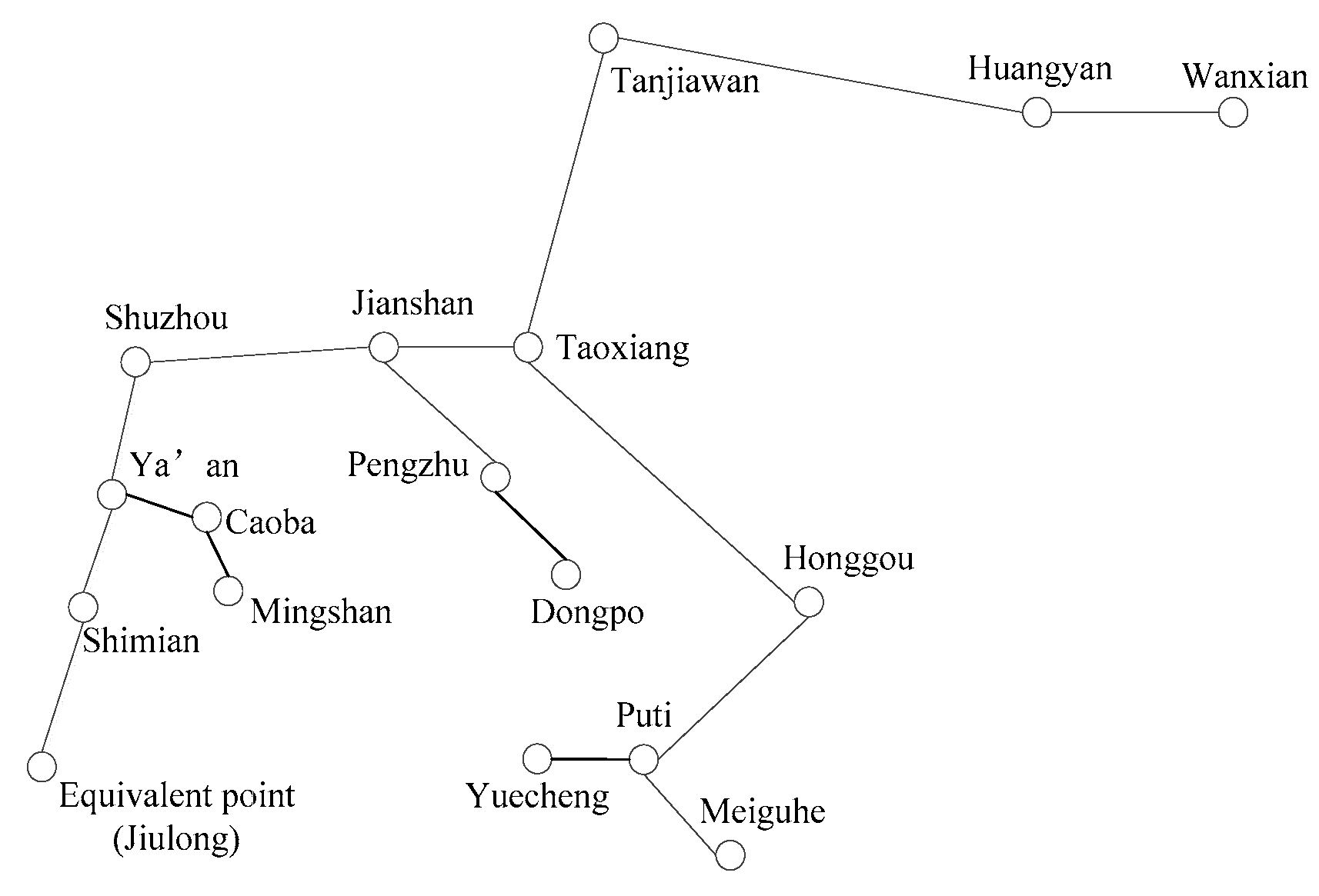
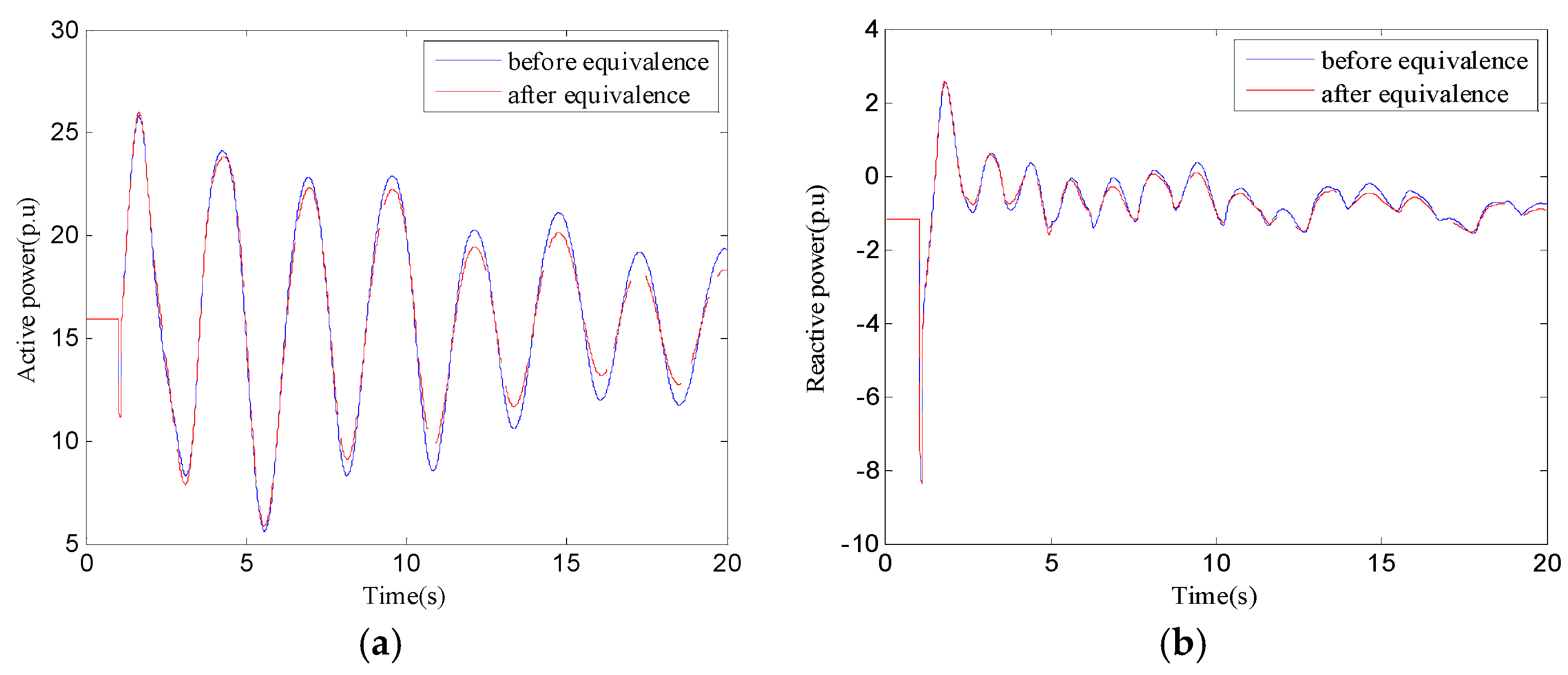
4.3. Equivalence with Simulation Data

Because it is a hydroelectric energy rich region, the hydropower capacity account for more than 60% of the total installed capacity in Sichuan. It is distributed in nearly 10 hydropower stations, a total of 23 hydroelectric generating units with a total capacity of 1578 MW in a certain area in Sichuan. The 5th order electromechanical transient generator and ZIP load models are represented in this area. Take the 500 kV hydropower channels in the area as an example. The proposed method in this paper is used to construct a dynamic equivalent model for the hydropower generator group. Parameters of equivalent model are shown in

Table 3. Parameters of equivalent model (p.u).

Parameter	Tj	xd	x′d	T′d0	Kv
Value	68.3137	0.5811	0.0455	15.3374	13.8422
Parameter	D	Ps0	Qs0	Np	Nq
Value	0.3093	0.7765	0.5897	0.5982	1.8078

. The dynamic response characteristics curves in the tie line of equivalent model and the negative load model are compared with the actual dynamic response characteristics for the hydropower generator group in Figure 8. Negative load is expressed as a constant impedance model which is commonly used in engineering. Moreover, the three phase short circuit occurred in 1 s in a 500 kV Shimian-Ya’an transmission line and broke this line in 1.1 s. The meaning of “before equivalence” indicates measurements obtained from the original system.

As can be seen from Figure 8, the dynamic response characteristics cannot be described accurately when the hydropower generator group is represented as a negative load. This is determined by the essential differences between generator and load models. On the other hand, the trends of dynamic responses are consistent before and after the equivalence, and the fitting rate is higher than the equivalence as a negative load.

The simple map representing the positions which are mentioned in this paper is shown in Figure 9. The partial results of power flow in internal system before and after equivalence are listed in

Table 4. The part of power flow results before and after equivalence (p.u).

Position	Type	Before Equivalence	After Equivalence	Relative Errors
Jiulong500–Shimian500	Active power	14.5465	14.55	0.024%
	Reactive power	−0.34845	−0.34935	0.25%
Jiulong500	Voltage amplitude	1.00641	1.00637	−0.0039%
Jianshan500–Pengzhu500	Active power	4.41634	4.41727	0.0047%
	Reactive power	1.41196	1.41087	0.079%
Jianshan500	Voltage amplitude	0.97591	0.97589	−0.0020%
Huangyan500–Wanxian500	Active power	15.90473	15.90617	0.0091%
	Reactive power	−1.177	−1.17682	0.015%
Huangyan500	Voltage amplitude	0.98683	0.98682	−0.001%
Meiguhe220–Puti220	Active power	0.53659	0.53659	0%
	Reactive power	0.49844	0.49845	0.0020%
Puti220	Voltage amplitude	0.9913	0.9913	0%
Caoba220–Mingshan220	Active power	0.29271	0.29271	0%
	Reactive power	−0.16314	−0.16313	0.0061%
Caoba220	Voltage amplitude	0.98993	0.98991	−0.0020%
grid	Frequency	1	1	0%

. It is shown that relative errors are within 0.3% and the system after equivalence can reflect the steady state operation.

The dynamic response characteristics curves on the interface between Huangyan in Sichuan and Wanxian in Chongqing before and after the equivalence are compared in Figure 10. As we can see from the figure, the transient response curves are similar and the system after equivalence can be used for transient stability analysis.

In order to verify the quality of the model reduction and parameter identification, the comparisons are done in before and after equivalence systems under other five faults, respectively. The fault descriptions and relative errors in the tie line are shown in

Table 5. Parameters of equivalent model (p.u).

Number	Fault Descriptions	Relative Errors
1	Three phase short circuit occurred in 1 s in a 500 kV Yuecheng-Puti transmission line and broke this line in 1.1 s	40.49
2	Three phase short circuit occurred in 1 s in a 500 kV Nantian-Dongpo transmission line and broke this line in 1.1 s	39.65
3	Three phase short circuit occurred in 1 s in a 500 kV Shuzhou-Danjing transmission line and broke this line in 1.1 s	34.17
4	Three phase short circuit occurred in 1 s in a 500 kV Ya’an-Jianshan transmission line and broke this line in 1.1 s	37.48
5	Three phase short circuit occurred in 1 s in a 500 kV Tanjiawan-Nanchong transmission line and broke this line in 1.1 s	28.56

.

As can be seen from Table 5, the maximum relative error is under No. 1 fault. Under No. 1 fault, for example, the dynamic responses characteristics curves in tie line and interface between Huangyan and Wanxian before and after equivalence are compared in Figure 11 and Figure 12. The oscillation frequency, amplitude and the shape of the curve trend are consistent according to Figure 11 and Figure 12. As can be seen in this section, the equivalent system keeps the dynamic characteristic of the original system and the effect of dynamic equivalence is good. The constructed model based on the proposed method can be applicable to a variety of situations and it keeps a certain robustness.

4.4. Equivalence with PMU Data

A small and medium hydropower generator group is connected to the grid through 220 kV and lower voltage substation, and connected to the main power grid by 500 kV substation. A disturbance occurred at 2:16:59 on October 1, 2015 in the 500 kV transmission line of Jiulong-Shimian in the Sichuan power grid. The fault waves from the 220 kV transmission line of Shaping-Jiulong were recorded by PMU. Based on the measurements and the equivalent method, the equivalent model of small and medium hydropower generator group in 220 kV Shaping area is constructed. The parameters of the model are shown in

Table 6. Parameters of equivalent model (p.u).

Parameter	Tj	xd	x′d	T′d0	Kv
Value	6.0684	0.5548	0.1475	1.6488	4.2420
Parameter	D	Ps0	Qs0	Np	Nq
Value	0.1982	1.1065	3.1636	0.8321	0.6005

while the transient response curves are shown in Figure 13.

The Figure 13 shows that the transient response curves have a good fitting. The small and medium hydropower generator group can be equivalent as a 3rd order electromechanical transient generator model with damping and a static characteristic load model considering voltage in a real-world situation.

In summary, the proposed equivalent method based on DMS-PSO is a good method to identify the parameters of the dynamic equivalent model of the hydropower generator group. It is not only fast and simple, but also accurate and practical. When a disturbance occurs, the dynamic equivalent model can be obtained, and this only relies on the phasor measurements. The proposed method has practical values for power system simulation.

5. Conclusions

In this paper, a measurement-based dynamic equivalent model and parameters identification method are proposed and verified for small and medium hydropower generator group. The optimal equivalent model parameters are obtained by combining the nonlinear 4th order Runge-Kutta method and DMS-PSO algorithm. The proposed method is verified respectively with the simulation and actual data. The dynamic responses with identified equivalent models are consistent with the actual dynamic responses, which demonstrate that the equivalent model can be used in the transient stability analysis. Besides, the proposed measurement-based equivalent model is more accurate and practical by modeling the small and medium hydropower generator group with the 3rd order generator model and a static load model than modeling it as a negative load. In the future, online application of the proposed approach will be studied in the actual power system.

References

1. Ni, Y.X.; Chen, S.S.; Zhang, B.L. Theory and Analysis of Dynamic Power System; Tsinghua University Press: Beijing, China, 2002; pp. 197–208. [Google Scholar]
2. Liu, Y.; Li, X.; Wang, Y. Research on small signal stability of power system with distributed small hydropower. In Proceedings of the Innovative Smart Grid Technologies-Asia, Tianjin, China, 21–24 May 2012; IEEE: New York, NY, USA, 2012. [Google Scholar]
3. Chang, Y.P.; Zhi, D.; Yang, D.J.; Zhao, H.S.; Zhang, Y.F.; Yang, H. An equivalent modeling for small and medium-sized hydropower generator group considering excitation and governor system. In Proceedings of the Power and Energy Engineering Conference, Hong Kong, China, 6–10 December 2014; IEEE: New York, NY, USA, 2014. [Google Scholar]
4. Xu, Z.D.; Sun, G.C.; Pan, R.R.; Xu, N.; Li, C.Q.; Ma, H.Z. An equivalent modeling for synthesis load of distributed network with small hydropower. In Proceedings of the 2014 4th International Workshop on Computer Science and Engineering, WCSE 2014, Dubai, UAE, 22–23 August 2014; Science and Engineering Institute: Bristol, UK, 2014. [Google Scholar]
5. Wang, M.; Wen, J.Y.; Hu, W.B.; Ruan, S.W.; Li, X.P.; Sun, J.B. A dynamic equivalent modeling for regional small hydropower generator group. Power Syst. Prot. Control 2013, 41, 1–9. [Google Scholar]
6. Joo, S.K.; Liu, C.C.; Choe, J.W. Enhancement of coherency identification techniques for power system dynamic equivalents. In Proceedings of the Power Engineering Society Summer Meeting, Vancouver, BC, Canada, 15–19 July 2001; IEEE: New York, NY, USA, 2001. [Google Scholar]
7. Oscar, Y.L.; Fette, M. Electromechanical identity recognition as alternative to the coherency identification. In Proceedings of the 39th International Universities Power Engineering Conference, Bristol, UK, 8 September 2004; IEEE: New York, NY, USA, 2004. [Google Scholar]
8. Nath, R.; Lamba, S.S. Development of coherency-based time-domain equivalent model using structure constraints. IEEE Proc. C Gener. Trans. Distrib. 1986, 133, 165–175. [Google Scholar] [CrossRef]
9. Ourari, M.L.; Dessaint, L.A.; Van-Que, D. Dynamic equivalent modeling of large power systems using structure preservation technique. IEEE Trans. Power Syst. 2006, 21, 1284–1295. [Google Scholar] [CrossRef]
10. Ourari, M.L.; Dessaint, L.A.; Van-Que, D. Generating units aggregation for dynamic equivalent of large power systems. In Proceedings of the IEEE Power Engineering Society General Meeting, Denver, CO, USA, 10 June 2004; IEEE: New York, NY, USA, 2004. [Google Scholar]
11. Ma, J.; Valle, R.J. Identification of dynamic equivalents preserving the internal modes. In Proceedings of the 2003 IEEE Bologna Power Tech Conference Proceedings, Bologna, Italy, 23–26 June 2004; IEEE: New York, NY, USA, 2004. [Google Scholar]
12. Price, W.W.; Ewart, D.N.; Gulachenski, E.M. Dynamic equivalents from on-line measurements. IEEE Trans. Power Appar. Syst. 1975, 94, 1349–1357. [Google Scholar] [CrossRef]
13. Azmy, A.M.; Erlich, I. Identification of dynamic equivalents for distribution power networks using recurrent ANNS. In Proceedings of the Power Systems Conference and Exposition, Bristol, UK, 10–13 October 2004; IEEE: New York, NY, USA, 2004. [Google Scholar]
14. Azmy, A.M.; Erlich, I.; Sowa, P. Artificial neural network-based dynamic equivalents for distribution systems containing active sources. IEEE Proc. Gener. Trans. Distrib. 2004, 151, 681–688. [Google Scholar] [CrossRef]
15. Rahim, A.H.M.A.; Al-Ramadhan, A.J. Dynamic equivalent of external power system and its parameter estimation through artificial neural network. Int. J. Electr. Power Energy Syst. 2002, 24, 113–120. [Google Scholar] [CrossRef]
16. Zali, S.M.; Milanovic, J.V. Dynamic equivalent model of Distribution Network Cell using Prony analysis and Nonlinear least square optimization. In Proceedings of the 2009 IEEE Bucharest Power Tech, Bucharest, Roman, 28 June 2009; IEEE: New York, NY, USA, 2009. [Google Scholar]
17. Zhou, Y.; Wang, K.; Zhang, B.H. A real-time dynamic equivalent solution for large interconnected power systems. In Proceedings of the Electric Utility Deregulation and Restructuring and Power Technologies, 2011 4th International Conference, Weihai, China, 6–9 July 2011; IEEE: New York, NY, USA, 2011. [Google Scholar]
18. Shi, H.B.; Hu, B.W.; Sun, J.T. Research on hydropower generator group equivalence and parameter identification based on PSASP calling and optimization algorithm. In Proceedings of the 2014 International Conference on Power and Energy, Shanghai, China, 29–30 November 2014; Taylor & Francis Group: London, UK, 2014. [Google Scholar]
19. Ju, P. Theory and Method of Power System Modeling; Science Press: Beijing, China, 2010; pp. 276–291. [Google Scholar]
20. Yang, Q.; Guan, L.; Wang, T.W. Influence on the performance of dynamic equivalence based on equivalent model. In Proceedings of the 24th Annual Conference Proceedings about Power System and Automation in China, Beijing, China, 10 October 2008.
21. Shi, D.; Tylavsky, D.J.; Koellner, M.; Logic, N.; Wheeler, D.E. Transmission line parameter identification using PMU measurements. Eur. Trans. Electr. Power 2011, 21, 1574–1588. [Google Scholar] [CrossRef]
22. Wu, S.X.; Zhang, B.M.; Wu, W.C.; Sun, H.B. Identification and validation for synchronous generator parameters based on recorded on-line disturbance data. Power Syst. Technol. 2012, 36, 87–93. [Google Scholar]
23. Chakhchoukh, Y.; Vittal, V.; Heydt, G.T. PMU based state estimation by integrating correlation. IEEE Trans. Power Syst. 2014, 29, 617–626. [Google Scholar] [CrossRef]
24. Jin, Y.Q.; Chen, Y.; Wang, D.M. Numerical Method; China Machine Press: Beijing, China, 2009; pp. 208–217. [Google Scholar]
25. Wang, W.H. Identification Based Dynamic Equivalents of Power Systems Interconnected with Three Areas. Master’s Thesis, Hohai University, Nanjing, China, 2007. [Google Scholar]
26. Zhang, N. Research on the Identification of Synchronous Generator Parameters Based on Phasor Measurement. Master’s Thesis, North China Electric Power University, Baoding, Hebei, China, 2007. [Google Scholar]
27. Shen, L.X. Parameters Identification for Power Load Models Based on Improved Particle Swarm Optimization Algorithm. Master’s Thesis, Dalian Maritime University, Dalian, China, 2013. [Google Scholar]
28. Kermedy, J.; Eberhart, R. Particle swarm optimization. In Proceedings of the IEEE International Conference on Neural Networks, Piscataway, NJ, USA, 27 November 1995; IEEE: New York, NY, USA, 1995. [Google Scholar]
29. Li, Z.K.; Chen, X.Y.; Yu, K. Hybrid particle swarm optimization for distribution network reconfiguration. Proc. CSEE 2008, 28, 35–41. [Google Scholar]
30. Zhu, Y.W.; Shi, X.C.; Dan, Y.Q.; Li, P.; Liu, W.Y.; Wei, D.B.; Fu, C. Application of PSO algorithm in global MPPT for PV array. Proc. CSEE 2012, 32, 42–48. [Google Scholar]
31. Zhao, S.Z.; Liang, J.J.; Suganthan, P.N. Dynamic multi-swarm particle swarm optimizer with local search for large scale global optimization. In Proceedings of the IEEE Congress on Evolutionary Computation, Hong Kong, China, 1–6 June 2008; IEEE: New York, NY, USA, 2008. [Google Scholar]
32. Liang, J.J.; Suganthan, P.N. Dynamic multi-swarm particle swarm optimizer. In Proceedings of the 2005 IEEE Swarm Intelligence Symposium, SIS 2005, New York, NY, USA, 8–10 June 2005; IEEE: New York, NY, USA, 2005. [Google Scholar]
Figure 1. Dynamic equivalent model structure.
Energies 09 00362 g001
Figure 2. The equivalent schematic diagram of hydropower generator group.
Energies 09 00362 g002
Figure 3. The schematic diagram of power in tie line.
Energies 09 00362 g003
Figure 4. Flow chart of parameter identification based on dynamic multi-swarm particle swarm optimizer (DMS-PSO) algorithm.
Energies 09 00362 g004
Figure 5. Residual error of power responses with different parameters.
Energies 09 00362 g005
Figure 6. (a) Active power curves based on identified parameters and actual parameters; (b) reactive power curves based on identified parameters and actual parameters.
Energies 09 00362 g006
Figure 7. (a) Active power curves based on identified parameters and actual parameters; (b) reactive power curves based on identified parameters and actual parameters.
Energies 09 00362 g007
Figure 8. (a) Active power curves about different model; (b) reactive power curves about different model.
Energies 09 00362 g008
Figure 9. The simple map.
Energies 09 00362 g009
Figure 10. (a) Active power curves between before and after equivalence; (b) reactive power curves between before and after equivalence.
Energies 09 00362 g010
Figure 11. (a) Active power curves between before and after equivalence; (b) reactive power curves between before and after equivalence.
Energies 09 00362 g011
Figure 12. (a) Active power curves between before and after equivalence; (b) reactive power curves between before and after equivalence.
Energies 09 00362 g012
Figure 13. (a) Active power curves between before and after equivalence; (b) Reactive power curves.
Energies 09 00362 g013