
A Least Squares Support Vector Machine Optimized by Cloud-Based Evolutionary Algorithm for Wind Power Generation Prediction


Abstract
:
1. Introduction
2. Methodology
2.1. Cloud-Based Evolutionary Algorithm
- (1)
- Evolving pattern. EP(Ex,En,He) is the evolving pattern described by the cloud model. Ex can be defined as the individual representing the good characteristics of ancestral inheritance. En is the evolving entropy to represent the range of mutation. He refers to the evolving hyper-entropy representing the evolving stability. Considering the parent individual (Ex) as the mother individual, we initialize the evolving entropy and the evolving hyper-entropy, then a population can be obtained from the cloud droplets generated by using the normal cloud generator. Therefore, the evolving pattern can be defined as the generating model of population.
- (2)
- Evolvement. Regarding the superior individual with better fitness value in the population as the mother individual, evolvement refers to the operation to generate a new population according to evolving pattern.
- (3)
- Mutation. Mutation is the operation where an excellent individual who abandons all or part of the father’s generation in the process of evolution, and can generate new individual on the basis of some certain strategies as the mother individual to produce the new population.
- (4)
- Evolving generation. A generation of the new community in the process of evolution is called an evolving generation.
- (5)
- Elite individual. Elite individuals, which are the most adaptable individuals in the evolvement process, can be classified into two types: the present elite individual and the cross generation elite individual. The present elite individual is the most adaptable individual in an evolving generation, and the cross generation elite individual is the most adaptable individual in different evolving generations. The successive common generation is that there is not cross generation elite continuously. Conversely, the successive excellent generations are that there are cross generation elites continuously.
- (6)
- Evolving strategy. Evolving strategy is the controlling strategy of evolvement in the process of evolution. Through the development of evolving strategy, two problems can be solved:
- (a)
- Local refinement. When there is a cross generation elite, the new extreme neighborhood can be found and the local refinement operation need to be carried out. The specific method is that the evolving range should be decreased (reduce En) and the stability should be augmented (reduce He). For instance, En and He can be set to the original values of 1/K, and K is the evolving coefficient greater than 1;
- (b)
- Local change (evolving variation). When the successive common generative reaches a certain threshold (λlocal), the algorithm may fall into a local optimal neighborhood. At this time, it needs to jump out of the local, and try to find a new local optimal. For instance, En and He can be L times larger than the original values, L is the evolving coefficient of variation. When the local optimal values of the function are very close, the evolutionary mutation can find the global optimal value in the local optimal values.
- (7)
- Mutation strategy. Mutation strategy is the controlling strategy of mutation operation in the process of evolution, which is the guarantee of getting rid of the local optimum. When the better individual cannot be obtained through several evolving generations and the evolving variation seems ineffective, the mutation operation needs to be conducted. The relationship between the threshold of local change and mutation is λglobal > λlocal. Mutation operation is used to find a new extreme area in the global scope. Correspondingly, the threshold of mutation can be defined as the threshold of global mutation (λglobal ).
- Step 1:
- The system is initialized to a set of random solutions, namely, the value of the individual in the community.
- Step 2:
- Calculate the fitness value of all individuals, and select the first m of the elite individuals, constituting the elite individual vector.
- Step 3:
- The first m individuals breed a population separately.
- Step 4:
- The elite individual is the optimal solution when the algorithm reaches the maximum evolving generation, otherwise the algorithm returns Step 2.
2.2. Least Squares Support Vector Machine
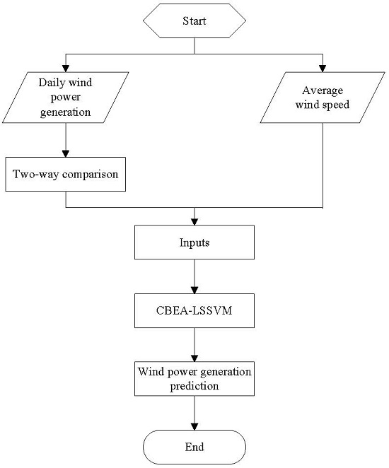
3. Approach of CBEA-LSSVM Model
- (1)
- Select the training set and the testing set.
- (2)
- Set the scope of the parameters (γ, σ2) to be trained.
- (3)
- The initial value of the evolutionary pattern (EP(Ex,En,He)) of CBEA-LSSVM can be determined according to Step (2), and En should be as large as possible, He ≥ 0.05; Set the scale of the community n, the size of the community richness m, the scale vector of the population V, the threshold of global mutation λglobal, the threshold of local mutation λlocal, the total evolving generation P, the evolving coefficient K, the evolving coefficient of variation L, and the fitness function f.
- (4)
- Generate the initial community using EP(Ex,En,He).
- (5)
- A series of prediction models can be obtained by placing all individual values of the community into Equation (7), and the prediction results can be attained by taking the sample as the input.
- (6)
- Calculate the fitness values of all individuals in the community by placing the predicted values into the fitness function, and eliminate the population in accordance with certain conditions.
- (7)
- Choose m elite individuals according to the size of fitness value and the requirement of control strategy, and record the successive common generation gc, the successive excellent generation ge.
- (8)
- Compare the size of ge and 0. If ge > 0, then it indicates that the individual is in the extreme neighborhood. Thus, the local refinement should be implemented, that is, to decrease the evolutionary scope (reduce En), to increase the stability (reduce He), and to expand the search accuracy and constancy.
- (9)
- If gc > λglobal, then the mutation operation should be performed.
- (10)
- If gc > λlocal, it shows that the individual can reach the local optimum. Then, the local change operation should be carried out by improving En and He.
- (11)
- Compute the new En and the new He, and the value of the elite individual regarded as Ex would be placed into the normal cloud generator to produce a new population.
- (12)
- Compare the evolving generation Q and the total evolving generation P. If Q < P, return to step (5). Otherwise, record the built group , and compare the fitness of all built groups to select the optimal individual. Then, is the optimal parameter of local refinement.
- (13)
- The optimal forecasting model can be obtained with the optimal parameter vector being brought into Equation (7).
- (14)
- The predicted values of the testing set can be gained by using the optimal forecasting model.
4. Case Study
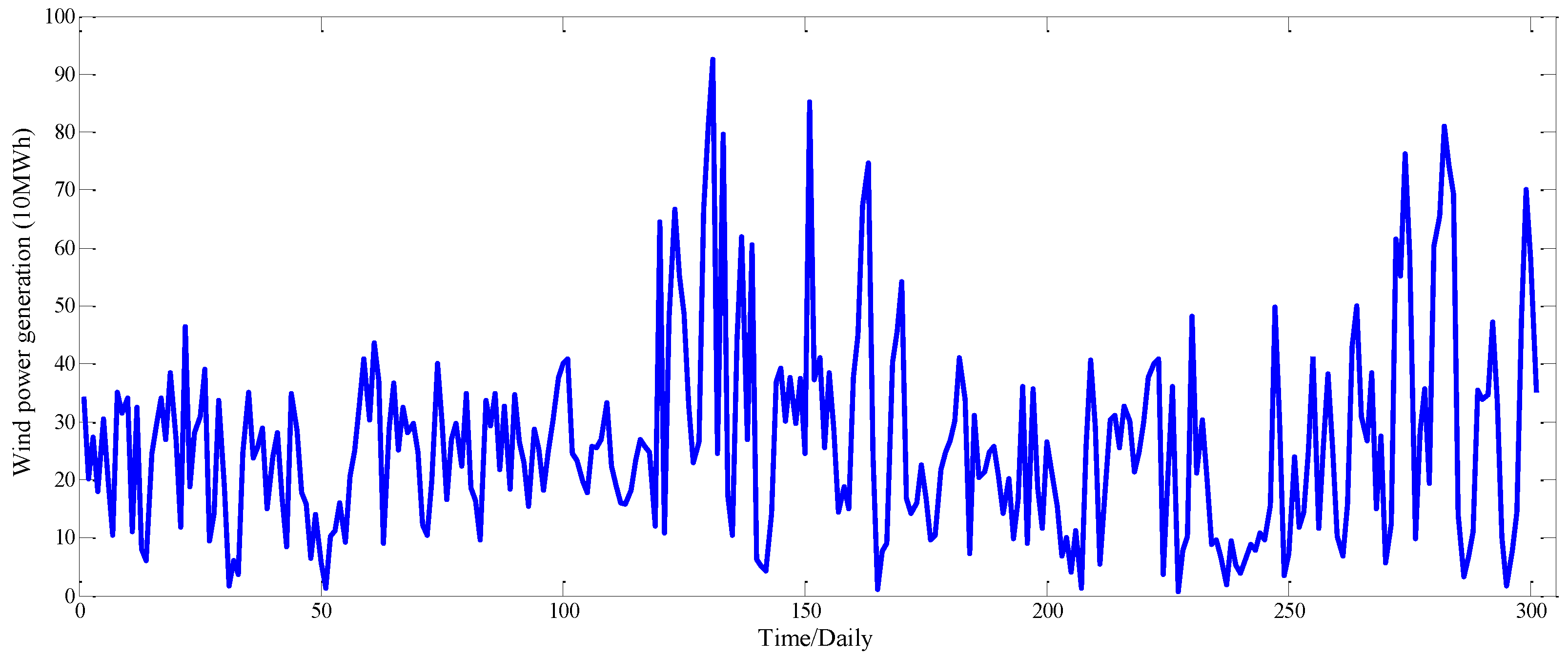
4.1. Data Sets
4.2. Data Preprocessing
4.2.1. Pretreatment of Abnormal Data
4.2.2. Data Normalization
4.3. Evaluation Criteria of Prediction Accuracy
4.4. Result Analysis of CBEA-LSSVM
4.5. Comparative Analysis
4.5.1. Analysis of CBEA-LSSVM with Various Parameters
4.5.2. Analysis of Different Forecasting Models
- (1)
- Among the three hybrid LSSVM models, the forecasting performance of CBEA-LSSVM is superior to GA-LSSVM and PSO-LSSVM in terms of the RMSE, MAE, MAPE and R2 evaluation criteria. For instance, the RMSE of CBEA-LSSVM is 1.3798, but the PSO-LSSVM and GA-LSSVM are 2.5701 and 2.8698, respectively. The coefficient of determination (R2) of CBEA-LSSVM is 0.9951, whereas those of the PSO-LSSVM and GA-LSSVM are 0.9883 and 0.9734, respectively.The primary reason may be that CBEA does not have the binary code, crossover and mutation operations of the genetic algorithm, but CBEA can produce a new population by using the normal cloud generator and adaptively control the position, scope (the scope of searching), and agglomeration degree (the particle size of refinement) of offspring through using entropy and hyper-entropy, which equips the LSSVM model with excellent ability to obtain the optimal solution quickly and avoid the issue of premature local convergence. Moreover, compared with the genetic algorithm, when the difference of the fitness value of most of the individuals in the population seems slight, the crossover operation will be powerless, and the algorithm can be easy to fall into local solutions and cannot be solved through the exchange. The sudden mutation can get rid of local convergence and jump out the local solution, but later variation may damage the constructive module which is helpful to form the optimal solution. However, CBEA can effectively avoid the drawbacks of GA since the evolving variation and mutation both utilize the historical search results. Hence, CBEA is superior to the genetic algorithm in the process of parameter optimization. Furthermore, based on real coding, CBEA and PSO both do not have crossover and mutation. The PSO approach determines the search according to the speed of particle, and the particles follow the current optimal particle to search in the current solution space. However, CBEA is a process where the individual has been produced and eliminated in each evolving generation, which not only embodies the idea of evolution, but also reflects the characteristics of human searching. Therefore, CBEA performs better than PSO in the process of parameter optimization;
- (2)
- The improved LSSVM models outperform the single LSSVM approach using the grid searching method and cross validation approach. For instance, the MAPE of CBEA-LSSVM, PSO-LSSVM, and GA-LSSVM are 8.10%, 19.71%, and 26.98%, but the MAPE of the single LSSVM is 31.11%. A possible explanation may be that the improved LSSVM model endows the LSSVM with better learning and generalization ability to gain the global optimal strategy easily and efficiently;
- (3)
- When compared to the ARMA model using only its own historical data, the improved LSSVM models and BPNN are more effective than the ARMA model representing the statistical models for wind power generation prediction.
4.5.3. Paired-Sample t-test
5. Conclusions
Acknowledgments
Author Contributions
Conflicts of Interest
References
- Zuluaga, C.D.; Álvarez, M.A.; Giraldo, E. Short-term wind speed prediction based on robust kalman filtering: An experimental comparison. Appl. Energy 2015, 156, 321–330. [Google Scholar] [CrossRef]
- Ait Maatallah, O.; Achuthan, A.; Janoyan, K.; Marzocca, P. Recursive wind speed forecasting based on hammerstein auto-regressive model. Appl. Energy 2015, 145, 191–197. [Google Scholar] [CrossRef]
- Foley, A.M.; Leahy, P.G.; Marvuglia, A.; McKeogh, E.J. Current methods and advances in forecasting of wind power generation. Renew. Energy 2012, 37, 1–8. [Google Scholar] [CrossRef] [Green Version]
- Saleh, A.E.; Moustafa, M.S.; Abo-Al-Ez, K.M.; Abdullah, A.A. A hybrid neuro-fuzzy power prediction system for wind energy generation. Int. J. Electr. Power Energy Syst. 2016, 74, 384–395. [Google Scholar] [CrossRef]
- Liu, H.; Tian, H.Q.; Li, Y.F. Four wind speed multi-step forecasting models using extreme learning machines and signal decomposing algorithms. Energy Convers. Manag. 2015, 100, 16–22. [Google Scholar] [CrossRef]
- Liu, H.; Tian, H.Q.; Li, Y.F.; Zhang, L. Comparison of four adaboost algorithm based artificial neural networks in wind speed predictions. Energy Convers. Manag. 2015, 92, 67–81. [Google Scholar] [CrossRef]
- Cassola, F.; Burlando, M. Wind speed and wind energy forecast through kalman filtering of numerical weather prediction model output. Appl. Energy 2012, 99, 154–166. [Google Scholar] [CrossRef]
- Ma, L.; Luan, S.; Jiang, C.; Liu, H.; Zhang, Y. A review on the forecasting of wind speed and generated power. Renew. Sustain. Energy Rev. 2009, 13, 915–920. [Google Scholar]
- Wang, L.; Dong, L.; Hao, Y.; Liao, X. Wind Power Prediction Using Wavelet Transform and Chaotic Characteristics. In Proceedings of the World Non-Grid-Connected Wind Power and Energy Conference (WNWEC 2009), Nanjing, China, 24–26 September 2009; pp. 1–5.
- Ewing, B.T.; Kruse, J.B.; Schroeder, J.L.; Smith, D.A. Time series analysis of wind speed using var and the generalized impulse response technique. J. Wind Eng. Ind. Aerodyn. 2007, 95, 209–219. [Google Scholar] [CrossRef]
- Bossanyi, E. Short-term wind prediction using kalman filters. Wind Eng. 1985, 9, 1–8. [Google Scholar]
- Liu, H.; Tian, H.Q.; Chen, C.; Li, Y.F. A hybrid statistical method to predict wind speed and wind power. Renew. Energy 2010, 35, 1857–1861. [Google Scholar] [CrossRef]
- Erdem, E.; Shi, J. Arma based approaches for forecasting the tuple of wind speed and direction. Appl. Energy 2011, 88, 1405–1414. [Google Scholar] [CrossRef]
- Liu, H.P.; Erdem, E.; Shi, J. Comprehensive evaluation of ARMA–GARCH(-M) approaches for modeling the mean and volatility of wind speed. Appl. Energy 2011, 88, 724–732. [Google Scholar] [CrossRef]
- Liu, H.; Tian, H.Q.; Li, Y.F. Comparison of two ARIMA-ANN and ARIMA-Kalman hybrid methods for wind speed prediction. Appl. Energy 2012, 98, 415–424. [Google Scholar] [CrossRef]
- Jiang, Y.; Song, Z.; Kusiak, A. Very short-term wind speed forecasting with bayesian structural break model. Renew. Energy 2013, 50, 637–647. [Google Scholar] [CrossRef]
- Sun, W.; Liu, M.; Liang, Y. Wind speed forecasting based on FEEMD and LSSVM optimized by the bat algorithm. Energies 2015, 8, 6585–6607. [Google Scholar] [CrossRef]
- Monfared, M.; Rastegar, H.; Kojabadi, H.M. A new strategy for wind speed forecasting using artificial intelligent methods. Renew. Energy 2009, 34, 845–848. [Google Scholar] [CrossRef]
- Li, G.; Shi, J. On comparing three artificial neural networks for wind speed forecasting. Appl. Energy 2010, 87, 2313–2320. [Google Scholar] [CrossRef]
- Tatinati, S.; Veluvolu, K.C.; Ang, W.T. Multistep prediction of physiological tremor based on machine learning for robotics assisted microsurgery. IEEE Trans. Cybern. 2015, 45, 328–339. [Google Scholar] [CrossRef] [PubMed]
- Yu, L.; Chen, H.; Wang, S.; Lai, K.K. Evolving least squares support vector machines for stock market trend mining. IEEE Trans. Evolut. Comput. 2009, 13, 87–102. [Google Scholar]
- Potter, C.W.; Negnevitsky, M. Very short-term wind forecasting for tasmanian power generation. IEEE Trans. Power Syst. 2006, 21, 965–972. [Google Scholar] [CrossRef]
- Sideratos, G.; Hatziargyriou, N. Using radial basis neural networks to estimate wind power production. In Proceedings of the IEEE Power Engineering Society General Meeting, Tampa, FL, USA, 24–28 June 2007; pp. 1–7.
- Pinson, P.; Kariniotakis, G. Conditional prediction intervals of wind power generation. IEEE Trans. Power Syst. 2010, 25, 1845–1856. [Google Scholar] [CrossRef] [Green Version]
- Kusiak, A.; Zhang, Z. Short-horizon prediction of wind power: A data-driven approach. IEEE Trans. Energy Convers. 2010, 25, 1112–1122. [Google Scholar] [CrossRef]
- Guo, Z.H.; Zhao, J.; Zhang, W.Y.; Wang, J.Z. A corrected hybrid approach for wind speed prediction in hexi corridor of China. Energy 2011, 36, 1668–1679. [Google Scholar] [CrossRef]
- De Giorgi, M.; Campilongo, S.; Ficarella, A.; Congedo, P. Comparison between wind power prediction models based on wavelet decomposition with least-squares support vector machine (LS-SVM) and artificial neural network (ANN). Energies 2014, 7, 5251–5272. [Google Scholar] [CrossRef]
- Yuan, X.; Chen, C.; Yuan, Y.; Huang, Y.; Tan, Q. Short-term wind power prediction based on LSSVM–GSA model. Energy Convers. Manag. 2015, 101, 393–401. [Google Scholar] [CrossRef]
- Sun, B.; Yao, H.-T. The short-term wind speed forecast analysis based on the PSO-LSSVM predict model. Power Syst. Prot. Control 2012, 40, 85–89. [Google Scholar]
- Wang, J.Z.; Wang, Y.; Jiang, P. The study and application of a novel hybrid forecasting model—A case study of wind speed forecasting in China. Appl. Energy 2015, 143, 472–488. [Google Scholar] [CrossRef]
- Mahjoob, M.J.; Abdollahzade, M.; Zarringhalam, R. Ga based optimized LSSVM forecasting of short term electricity price in competitive power markets. In Proceedings of 2008 3rd IEEE Conference on Industrial Electronics and Applications, Siem Reap, Cambodia, 18–20 June 2017; pp. 73–78.
- Jung, H.C.; Kim, J.S.; Heo, H. Prediction of building energy consumption using an improved real coded genetic algorithm based least squares support vector machine approach. Energy Build. 2015, 90, 76–84. [Google Scholar] [CrossRef]
- Zhang, G.W.; He, R.; Liu, Y.; Li, D.Y.; Chen, G.S. An evolutionary algorithm based on cloud model. Chin. J. Comput. 2008, 31, 1082–1090. [Google Scholar] [CrossRef]
- Li, D.Y.; Liu, C.Y.; Du, Y.; Han, X. Artificial intelligence with uncertainty. J. Soft. 2004, 15, 1583–1594. [Google Scholar]
- Kusiak, A.; Zheng, H.; Song, Z. Models for monitoring wind farm power. Renew. Energy 2009, 34, 583–590. [Google Scholar] [CrossRef]
- Xiao, B.; Xu, X.; Song, K.; Bai, Y.; Li, J.F. Abnormal data identification and treatment in spatial electric load forecasting. J. Northeast Dianli Univ. 2013, 33, 45–50. [Google Scholar]
- Suykens, J.A.K.; Vandewalle, J. Recurrent least squares support vector machines. IEEE Trans. Circuits Syst. I Fundam. Theory Appl. 2000, 47, 1109–1114. [Google Scholar] [CrossRef]
- Ahmed, H.; Ushirobira, R.; Efimov, D.; Tran, D.; Sow, M.; Payton, L.; Massabuau, J.C. A fault detection method for automatic detection of spawning in oysters. IEEE Trans. Control Syst. Technol. 2016, 34, 1140–1147. [Google Scholar] [CrossRef]
- Wei, X. Statistical Analysis and Spss Application, 3rd ed.; China Renmin University Press: Beijing, China, 2011. [Google Scholar]


| Parameters | Values | Parameters | Values |
|---|---|---|---|
| Entropy (En) | Total evolving generation (P) | 20 | |
| Hyper-entropy (He) | Evolving coefficient (K) | 10 | |
| Scale of the community (n) | 100 | Evolving coefficient of variation (L) | |
| Threshold of global mutation (λglobal) | 6 | Size of the community richness (m) | 10 |
| Threshold of local mutation (λlocal) | 2 |
| CBEA-LSSVM | Indices | |||
|---|---|---|---|---|
| RMSE (10 MWh) | MAE(10 MWh) | MAPE (%) | R2 | |
| En = [0.618,0.618] P = 20 | 2.2762 | 2.1491 | 20.17 | 0.9910 |
| En = [0.618,0.618] P = 10 | 1.9093 | 1.7007 | 14.51 | 0.9932 |
| En = [61.8,61.8] P = 10 | 1.7266 | 1.6182 | 13.59 | 0.9939 |
| En = [61.8,61.8] P = 20 | 1.3798 | 1.1281 | 8.10 | 0.9951 |
| Parameters | Forecasting Methods | |||
|---|---|---|---|---|
| CBEA-LSSVM | PSO-LSSVM | GA-LSSVM | LSSVM | |
| γ | 0.0583 | 3.6119 | 12.8347 | 10.2634 |
| σ2 | 0.3376 | 0.3247 | 1.0216 | 0.1368 |
| Computing Time (s) | Forecasting Methods | |||||
|---|---|---|---|---|---|---|
| CBEA-LSSVM | PSO-LSSVM | GA-LSSVM | LSSVM | BPNN | ARMA | |
| Time | 8.901 | 190.137 | 117.41 | 4.992 | 13.077 | 0.925 |
| Evolving Generation | γ | σ2 | Evolving Generation | γ | σ2 |
|---|---|---|---|---|---|
| 1 | 0.0884 | 0.3756 | 11 | 0.0588 | 0.3386 |
| 2 | 0.0872 | 0.3716 | 12 | 0.0587 | 0.3384 |
| 3 | 0.0803 | 0.3651 | 13 | 0.0585 | 0.3382 |
| 4 | 0.0782 | 0.3657 | 14 | 0.0584 | 0.3383 |
| 5 | 0.0702 | 0.3645 | 15 | 0.0583 | 0.3380 |
| 6 | 0.0622 | 0.3635 | 16 | 0.0582 | 0.3378 |
| 7 | 0.0604 | 0.3609 | 17 | 0.0583 | 0.3376 |
| 8 | 0.0596 | 0.3576 | 18 | 0.0583 | 0.3376 |
| 9 | 0.0590 | 0.3514 | 19 | 0.0583 | 0.3376 |
| 10 | 0.0589 | 0.3387 | 20 | 0.0583 | 0.3376 |
| Indices | Forecasting Approaches | |||||
|---|---|---|---|---|---|---|
| CBEA-LSSVM | PSO-LSSVM | GA-LSSVM | LSSVM | BPNN | ARMA | |
| RMSE (10 MWh) | 1.3798 | 2.1846 | 2.8698 | 3.4578 | 3.8507 | 5.3420 |
| MAE (10 MWh) | 1.1281 | 2.0612 | 2.6423 | 3.2496 | 3.4200 | 3.9939 |
| MAPE (%) | 8.10 | 19.71 | 26.98 | 31.11 | 33.46 | 46.12 |
| 0.9951 | 0.9883 | 0.9734 | 0.8875 | 0.8579 | 0.8253 | |
| Pairs | Paired Differences (Wind Power Generation Forecasted by Single LSSVM Model Minus Wind Power Generation Forecasted by Hybrid Model) | Probability (Two-Tailed) | |||
|---|---|---|---|---|---|
| Mean | Standard Deviation | 95% Confidence Interval of the Difference | |||
| Lower | Upper | ||||
| Pair 1: LSSVM–CBEA | −1.5119915 | 4.1382006 | −2.4270228 | −0.5969602 | 0.001 |
| Pair 2: LSSVM–GA | −1.4031577 | 3.9581253 | −2.2783711 | −0.5279443 | 0.002 |
| Pair 3: LSSVM–PSO | −1.4968162 | 4.0001929 | −2.3813315 | −0.6123010 | 0.001 |
© 2016 by the authors; licensee MDPI, Basel, Switzerland. This article is an open access article distributed under the terms and conditions of the Creative Commons Attribution (CC-BY) license (http://creativecommons.org/licenses/by/4.0/).
Share and Cite
Wu, Q.; Peng, C. A Least Squares Support Vector Machine Optimized by Cloud-Based Evolutionary Algorithm for Wind Power Generation Prediction. Energies 2016, 9, 585. https://doi.org/10.3390/en9080585
Wu Q, Peng C. A Least Squares Support Vector Machine Optimized by Cloud-Based Evolutionary Algorithm for Wind Power Generation Prediction. Energies. 2016; 9(8):585. https://doi.org/10.3390/en9080585
Chicago/Turabian StyleWu, Qunli, and Chenyang Peng. 2016. "A Least Squares Support Vector Machine Optimized by Cloud-Based Evolutionary Algorithm for Wind Power Generation Prediction" Energies 9, no. 8: 585. https://doi.org/10.3390/en9080585