
A Hybrid Multi-Step Model for Forecasting Day-Ahead Electricity Price Based on Optimization, Fuzzy Logic and Model Selection


Abstract
:
1. Introduction
- ➢
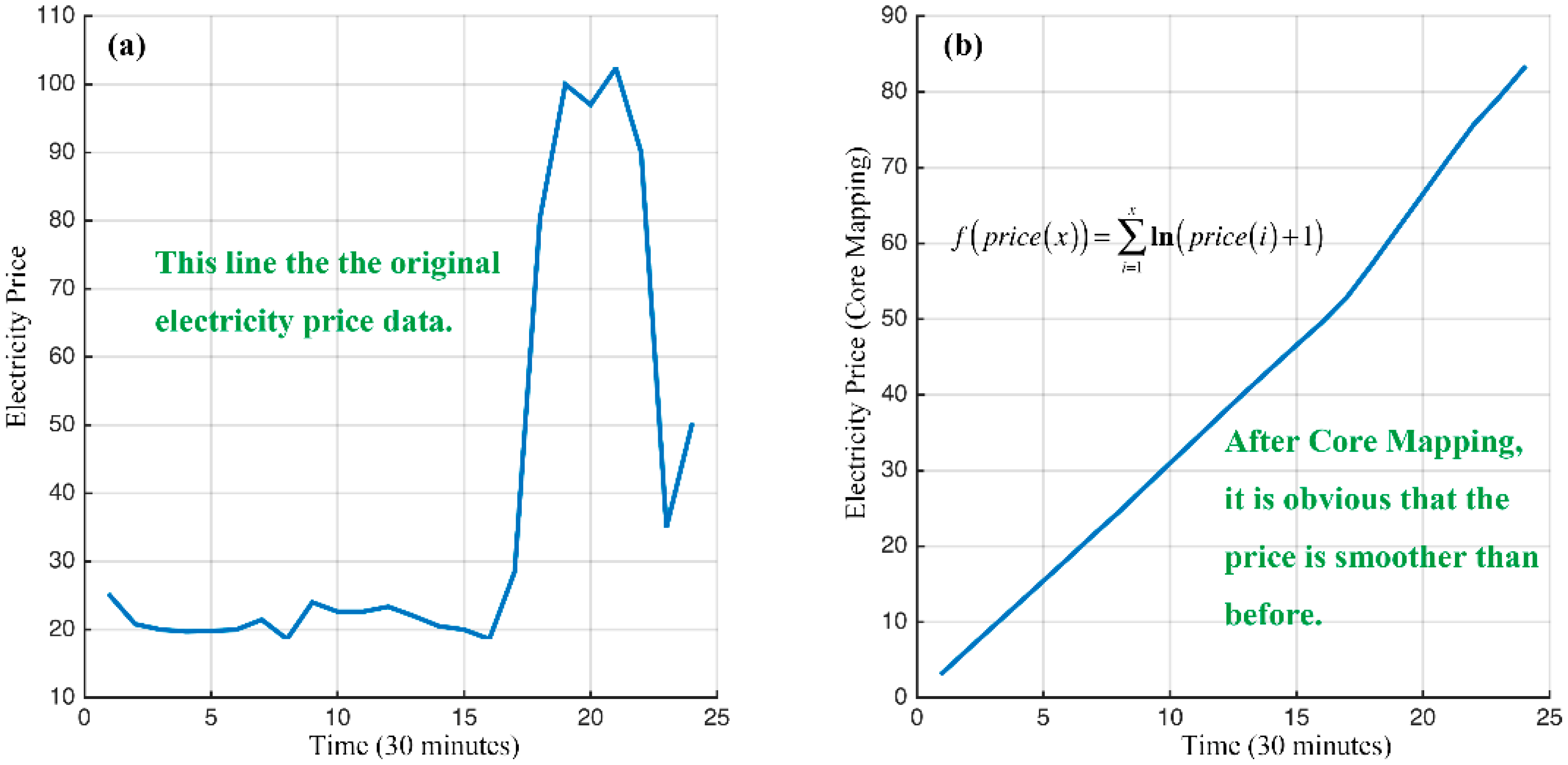
- We successfully overcome the volatility of the electricity price through the CM method.
- ➢
- Improvement from reducing the volatility is obvious during the test period.
- ➢
- Self-organizing map (SOM) is assigned to divide the original data into three parts: low, medium and high.
- ➢
- Divided price is weighted by the PSO algorithm and performs well during forecasting.
- ➢
- SR is based on three new defined criteria and effectively selects the forecasting model.
2. Self-Organizing-Map
3. Core Mapping-Particle Swarm Optimization-Core Mapping with Self-Organizing-Map and Fuzzy Set-Selection Rule for Electricity Price Forecasting
3.1. Core Idea of This Paper
- ■
- IF price(i) IS High price, THEN price(i) equals price(i) × Highweight;
- ■
- IF price(i) IS Medium price, THEN price(i) equals price(i) × Mediumweight; and
- ■
- IF price(i) IS Low price, THEN price(i) equals price(i) × Lowweight.
3.2. Basic Pre-Process
3.3. Core Mapping Method
3.4. Swarm Optimization Algorithm-Core Mapping with Self-Organizing Map and Fuzzy (Particle Swarm Optimization-Core Mapping with Self-Organizing-Map and Fuzzy Set) Method
3.4.1. Forecasting Rules
- (1)
- A previous month’s data are used to forecast the price of the target day.
- (2)
- There is only the historical electricity price considered in this paper (without data of demand or environmental data (for the environmental data, we do not find the corresponding dataset (24 h in one day))).
- (3)
- All forecasting results are day-ahead forecasting, and the forecasting mode is shown in Figure 4.
3.4.2. Classification of Price with Self-Organizing Map and Fuzzy Logic
3.4.3. Applying of Swarm Optimization Algorithm Algorithm
3.5. Selection Rule Based on Forecasting Nature of Radial Basis Function Network
- RBF Network in Forecasting
| Algorithm 1 Pseudo code of forecasting the electricity price of the ith day using the CM-PCMwSF-SR model. | |
| P: The electricity price series | |
| T: Number of time points in one-day electricity price series. | |
| Iter: Number of iterations. | |
| t = 1. | |
| 1 | Assign Equations (6) and (7) to pre-process P |
| 2 | According to CM method, map P to PCM |
| 3 | Divide PCM into T subseries and denote them by PCM1, PCM2, …, PCMT |
| 4 | According to CM method, map P to PPCM |
| 5 | Divide PPCM into T subseries and denote them by PPCM1, PPCM2, …, PPCMT |
| 6 | While t < T + 1 |
| 7 | Assign Pcmt and RBFN, forecast the time t of electricity price of ith day and denote it by pfcm(i, t). |
| 8 | Assign Ppcmt and RBFN, forecast the time t of electricity price of ith day and denote it by pfpcm(i, t). |
| 9 | t = t + 1 |
| 10 | End |
| 11 | Calculate ICP-F(i; pfcm) and ICP-F(i; pfpcm) |
| 12 | IF ICP-F(i; pfcm) > ICP-F(i; pfpcm) |
| 13 | Pf = pfcm |
| 14 | Else |
| 15 | Pf = pfpcm |
| 16 | End |
| 17 | Return Pf |
3.6. Forecasting Principle and Evaluation Criteria
4. Data Analyses and Numerical Results
4.1. Study of Case 1
4.2. Study of Case 2
4.3. Study of Case 3
4.4. Study of Cases 4–6
4.5. Comparison Study
- (a)
- PSO is a better selection to optimize the weights of low and high electricity prices than GA because CM-PCMwSF-SR has better overall forecasting effectiveness than CM-GCMwSF-SR.
- (b)
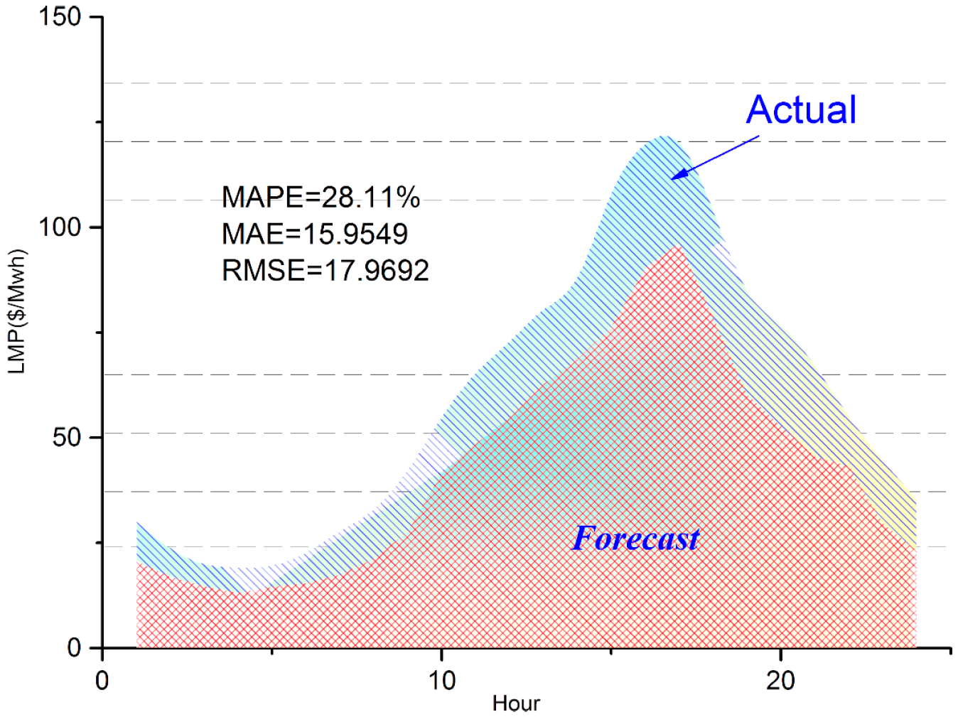
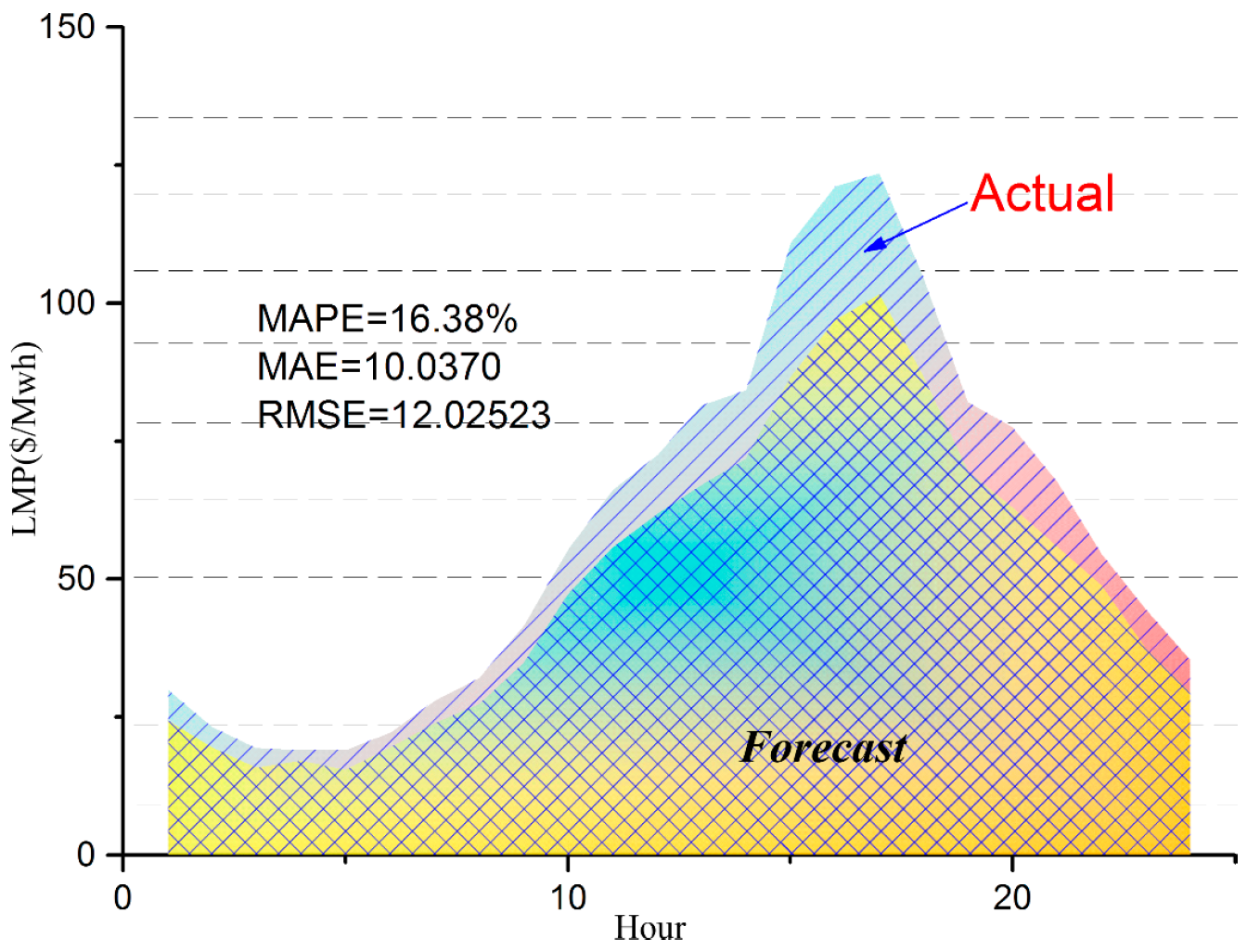
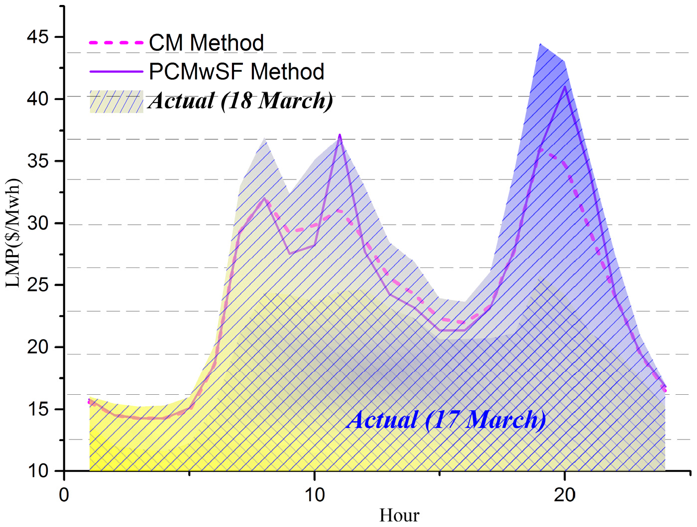
- PCMwSF and CM have ability to improve the forecasting accuracy.
- (c)
- The electricity price of autumn can be predicted more precisely.
- (d)
- Although some literature regard the electricity demand as features to predict electricity price, adding the electricity demand data as a feature cannot help to improve forecasting effectiveness of prices in this paper (forecasting results are similar in Table 7).
- (1)
- The proposed model mostly concentrates on reducing the volatility of electricity price for a higher accuracy, which means the electricity demand is not important compared to the pre-processed electricity price.
- (2)
- Model performance under specific conditions should be analyzed and understood and incremental improvements made based on knowledge gained. Moghram and Rahman review five short-term load forecasting methods:
- (i)
- multiple linear regression;
- (ii)
- time series;
- (iii)
- general exponential smoothing;
- (iv)
- state space and Kallman filter; and
- (v)
- knowledge-based approach.
5. Conclusions
Acknowledgments
Author Contributions
Conflicts of Interest
Abbreviations
| RBFN | Radial basis function network |
| PCMwSF | Particle swarm optimization-core mapping with self-organizing-map and fuzzy set |
| CM | Core mapping |
| SR | Selection rule |
| MI | Mutual information |
| CNN | Composite neural network |
| SVM | Support vector machine |
| ARMAX | Auto-regressive moving average with external input |
| MS-GARCH | Markov-switching generalized autoregressive conditional heteroskedasticity |
| DCT | Discrete cosine transforms |
| FFNN | Feed-forward neural network |
| CFNN | Cascade-forward neural network |
| GRNN | Generalized regression neural network |
| PSO | Particle swarm optimization |
| PCPF | Panel cointegration and particle filter |
| WT | Wavelet transform |
| ARIMA | Autoregressive integrated moving average |
| LSSVM | Least squares support vector machine |
| CLSSVM | Chaotic least squares support vector machine |
| EGARCH | Exponential generalized autoregressive conditional heteroskedastic |
| ARMA | Autoregressive moving average |
| GARCH | Generalized autoregressive conditional heteroskedasticity |
| ARMA-GARCH-M | ARMA-GARCH-in-mean |
| ARFIMA | Auto-regressive fractionally integrated moving average |
| ANN | Artificial neural network |
| ELM | Extreme learning machine |
| PIs | Prediction intervals |
| RNN | Recurrent neural network |
| PNN | Probabilistic neural network |
| HNES | Hybrid neuro-evolutionary system |
| PCA | Principal component analysis |
| MLF | Multi-layer feedforward |
| BPNN | Backward propagation neural network |
| ENN | Elman neural network |
| GA | Genetic algorithm |
References
- Sáez, Á.E. Modeling electricity prices: International evidence. In Proceedings of the European Financial Management Association (EFMA), London, UK, 26–29 June 2002; pp. 2–34.
- Liu, H.; Shi, J. Applying ARMA–GARCH approaches to forecasting short-term electricity prices. Energy Econ. 2013, 37, 152–166. [Google Scholar] [CrossRef]
- García-Martos, C.; Rodríguez, J.; Sánchez, M.J. Forecasting electricity prices and their volatilities using Unobserved Components. Energy Econ. 2011, 33, 1227–1239. [Google Scholar] [CrossRef] [Green Version]
- Keynia, F. A new feature selection algorithm and composite neural network for electricity price forecasting. Eng. Appl. Artif. Intell. 2012, 25, 1687–1697. [Google Scholar] [CrossRef]
- Yan, X.; Chowdhury, N.A. Mid-term electricity market clearing price forecasting: A hybrid LSSVM and ARMAX approach. Int. J. Electr. Power Energy Syst. 2013, 53, 20–26. [Google Scholar] [CrossRef]
- Yan, X.; Chowdhury, N.A. Mid-term electricity market clearing price forecasting utilizing hybrid support vector machine and auto-regressive moving average with external input. Int. J. Electr. Power Energy Syst. 2014, 63, 64–70. [Google Scholar] [CrossRef]
- Cifter, A. Forecasting electricity price volatility with the Markov-switching GARCH model: Evidence from the Nordic electric power market. Electr. Power Syst. Res. 2013, 102, 61–67. [Google Scholar] [CrossRef]
- Anbazhagan, S.; Kumarappan, N. Day-ahead deregulated electricity market price classification using neural network input featured by DCT. Int. J. Electr. Power Energy Syst. 2012, 37, 103–109. [Google Scholar] [CrossRef]
- Anbazhagan, S.; Kumarappan, N. A neural network approach to day-ahead deregulated electricity market prices classification. Electr. Power Syst. Res. 2012, 86, 140–150. [Google Scholar] [CrossRef]
- Anbazhagan, S.; Kumarappan, N. Day-ahead deregulated electricity market price forecasting using neural network input featured by DCT. Energy Convers. Manag. 2014, 78, 711–719. [Google Scholar] [CrossRef]
- Lei, M.; Feng, Z. A proposed grey model for short-term electricity price forecasting in competitive power markets. Int. J. Electr. Power Energy Syst. 2012, 43, 531–538. [Google Scholar] [CrossRef]
- Li, X.R.; Yu, C.W.; Ren, S.Y.; Chiu, C.H.; Meng, K. Day-ahead electricity price forecasting based on panel cointegration and particle filter. Electr. Power Syst. Res. 2013, 95, 66–76. [Google Scholar] [CrossRef]
- Zhang, J.; Tan, Z.; Yang, S. Day-ahead electricity price forecasting by a new hybrid method. Comput. Ind. Eng. 2012, 63, 695–701. [Google Scholar] [CrossRef]
- Zhang, J.; Tan, Z. Day-ahead electricity price forecasting using WT, CLSSVM and EGARCH model. Int. J. Electr. Power Energy Syst. 2013, 45, 362–368. [Google Scholar] [CrossRef]
- Chaâbane, N. A hybrid ARFIMA and neural network model for electricity price prediction. Int. J. Electr. Power Energy Syst. 2014, 55, 187–194. [Google Scholar] [CrossRef]
- Babu, C.N.; Reddy, B.E. A moving-average filter based hybrid ARIMA–ANN model for forecasting time series data. Appl. Soft Comput. 2014, 23, 27–38. [Google Scholar] [CrossRef]
- Shrivastava, N.A.; Panigrahi, B.K. A hybrid wavelet-ELM based short term price forecasting for electricity markets. Int. J. Electr. Power Energy Syst. 2014, 55, 41–50. [Google Scholar] [CrossRef]
- Shayeghi, H.; Ghasemi, A. Day-ahead electricity prices forecasting by a modified CGSA technique and hybrid WT in LSSVM based scheme. Energy Convers. Manag. 2013, 74, 482–491. [Google Scholar] [CrossRef]
- Khosravi, A.; Nahavandi, S.; Creighton, D. A neural network-GARCH-based method for construction of Prediction Intervals. Electr. Power Syst. Res. 2013, 96, 185–193. [Google Scholar] [CrossRef]
- Khosravi, A.; Nahavandi, S.; Creighton, D. Quantifying uncertainties of neural network-based electricity price forecasts. Appl. Energy 2013, 112, 120–129. [Google Scholar] [CrossRef]
- Khosravi, A.; Nahavandi, S. Effects of type reduction algorithms on forecasting accuracy of IT2FLS models. Appl. Soft Comput. 2014, 17, 32–38. [Google Scholar] [CrossRef]
- Bordignon, S.; Bunn, D.W.; Lisi, F.; Nan, F. Combining day-ahead forecasts for British electricity prices. Energy Econ. 2013, 35, 88–103. [Google Scholar] [CrossRef]
- Grimes, D.; Ifrim, G.; O’Sullivan, B.; Simonis, H. Analyzing the impact of electricity price forecasting on energy cost-aware scheduling. Sustain. Comput. Inform. Syst. 2014, 4, 276–291. [Google Scholar] [CrossRef]
- Nowotarski, J.; Raviv, E.; Trück, S.; Weron, R. An empirical comparison of alternative schemes for combining electricity spot price forecasts. Energy Econ. 2014, 46, 395–412. [Google Scholar] [CrossRef]
- Sharma, V.; Srinivasan, D. A hybrid intelligent model based on recurrent neural networks and excitable dynamics for price prediction in deregulated electricity market. Eng. Appl. Artif. Intell. 2013, 26, 1562–1574. [Google Scholar] [CrossRef]
- Dev, P.; Martin, M.A. Using neural networks and extreme value distributions to model electricity pool prices: Evidence from the Australian National Electricity Market 1998–2013. Energy Convers. Manag. 2014, 84, 122–132. [Google Scholar] [CrossRef]
- Wang, J.; Zhang, W.; Li, Y.; Wang, J.; Dang, Z. Forecasting wind speed using empirical mode decomposition and Elman neural network. Appl. Soft Comput. 2014, 23, 452–459. [Google Scholar] [CrossRef]
- Hickey, E.; Loomis, D.G.; Mohammadi, H. Forecasting hourly electricity prices using ARMAX-GARCH models: An application to MISO hubs. Energy Econ. 2012, 34, 307–315. [Google Scholar] [CrossRef]
- Christensen, T.M.; Hurn, A.S.; Lindsay, K.A. Forecasting spikes in electricity prices. Int. J. Forecast. 2012, 28, 400–411. [Google Scholar] [CrossRef]
- Amjady, N.; Keynia, F. A new prediction strategy for price spike forecasting of day-ahead electricity markets. Appl. Soft Comput. J. 2011, 11, 4246–4256. [Google Scholar] [CrossRef]
- Dudek, G. Multilayer perceptron for GEFCom2014 probabilistic electricity price forecasting. Int. J. Forecast. 2016, 32, 1057–1060. [Google Scholar] [CrossRef]
- Panapakidis, I.P.; Dagoumas, A.S. Day-ahead electricity price forecasting via the application of artificial neural network based models. Appl. Energy 2016, 172, 132–151. [Google Scholar] [CrossRef]
- Feijoo, F.; Silva, W.; Das, T.K. A computationally efficient electricity price forecasting model for real time energy markets. Energy Convers. Manag. 2016, 113, 27–35. [Google Scholar] [CrossRef]
- Abedinia, O.; Amjady, N.; Shafie-Khah, M.; Catalão, J.P.S. Electricity price forecast using Combinatorial Neural Network trained by a new stochastic search method. Energy Convers. Manag. 2015, 105, 642–654. [Google Scholar] [CrossRef]
- He, K.; Xu, Y.; Zou, Y.; Tang, L. Electricity price forecasts using a Curvelet denoising based approach. Phys. A Stat. Mech. Its Appl. 2015, 425, 1–9. [Google Scholar] [CrossRef]
- Ziel, F.; Steinert, R.; Husmann, S. Efficient modeling and forecasting of electricity spot prices. Energy Econ. 2015, 47, 98–111. [Google Scholar] [CrossRef]
- Hong, Y.Y.; Wu, C.P. Day-ahead electricity price forecasting using a hybrid principal component analysis network. Energies 2012, 5, 4711–4725. [Google Scholar] [CrossRef]
- Cerjan, M.; Matijaš, M.; Delimar, M. Dynamic hybrid model for short-term electricity price forecasting. Energies 2014, 7, 3304–3318. [Google Scholar] [CrossRef]
- Monteiro, C.; Fernandez-Jimenez, L.A.; Ramirez-Rosado, I.J. Explanatory information analysis for day-ahead price forecasting in the Iberian electricity market. Energies 2015, 8, 10464–10486. [Google Scholar] [CrossRef]
- Jónsson, T.; Pinson, P.; Nielsen, H.A.; Madsen, H. Exponential smoothing approaches for prediction in real-time electricity markets. Energies 2014, 7, 3710–3732. [Google Scholar] [CrossRef] [Green Version]
- Weron, R. Electricity price forecasting: A review of the state-of-the-art with a look into the future. Int. J. Forecast. 2014, 30, 1030–1081. [Google Scholar] [CrossRef]
- Wikipedia File: Synapse Self-Organizing Map. Available online: http://en.wikipedia.org/wiki/File:Synapse_Self-Orga (accessed on 1 August 2016).
- Shafie-Khah, M.; Moghaddam, M.P.; Sheikh-El-Eslami, M.K. Price forecasting of day-ahead electricity markets using a hybrid forecast method. Energy Convers. Manag. 2011, 52, 2165–2169. [Google Scholar] [CrossRef]
- Zadeh, L.A. Fuzzy logic. Computer 1988, 21, 83–93. [Google Scholar] [CrossRef]
- Zadeh, L.A. Fuzzy sets. Inf. Control 1965, 8, 338–353. [Google Scholar] [CrossRef]
- Zhao, J.; Guo, Z.H.; Su, Z.Y.; Zhao, Z.Y.; Xiao, X.; Liu, F. An improved multi-step forecasting model based on WRF ensembles and creative fuzzy systems for wind speed. Appl. Energy 2016, 162, 808–826. [Google Scholar] [CrossRef]
- Wang, Z.; Liu, F.; Wu, J.; Wang, J. A hybrid forecasting model based on bivariate division and a backpropagation artificial neural network optimized by chaos particle swarm optimization for day-ahead electricity price. Abstr. Appl. Anal. 2014, 2014. [Google Scholar] [CrossRef]
- Kohonen, T. Self-organized formation of topologically correct feature maps. Biol. Cybern. 1982, 43, 59–69. [Google Scholar] [CrossRef]
- Ultsch, A. Emergence in Self Organizing Feature Maps. In Proceedings of the 6th International Workshop on Self-Organizing Maps, Bielefeld, Germany, 3–6 September 2007.
- Kohonen, T. Self-Organizing Maps; Springer-Verlag New York, Inc.: New York, NY, USA, 1997. [Google Scholar]
- Moghram, I.S.; Rahman, S. Analysis and evaluation of five short-term load forecasting techniques. IEEE Trans. Power Syst. 1989, 4, 1484–1491. [Google Scholar] [CrossRef]


| Case | Forecasted Data | Remarks |
|---|---|---|
| 1 | 26 June 2002 | Test data 1 |
| 2 | 28 June 2002 | Test data 2 |
| 3 | 18–22 March 2002 | Spring week |
| 4 | 24–28 June 2002 | Summer week |
| 5 | 23–27 September 2002 | Autumn week |
| 6 | 23–27 December 2002 | Winter week |
| Hour | Optimized Lowweight | Optimized Highweight | Optimized Ind | vop | Accuracy of Price Forecasting in 25 June with Optimized Weight | Actual Price | The Forecasting Price | The MAPE in Forecasting | Lowprice | Mediumprice | Highprice | |||
|---|---|---|---|---|---|---|---|---|---|---|---|---|---|---|
| Lower Limit | Upper Limit | Lower Limit | Upper Limit | Lower Limit | Upper Limit | |||||||||
| 1 | 1.05 | 1.05 | 3.00 × 10⁻⁷ | 3 × 10⁻⁵ | 0.009871573 | 30.042584 | 28.88083544 | 0.038670061 | 13.35 | 16.38 | 16.47 | 19.99 | 20.33 | 21.77 |
| 2 | 0.9 | 1.05 | 1.17 × 10⁻⁶ | 0.00175 | 0.000669503 | 23.227286 | 22.82923041 | 0.017137413 | 6.21 | 11.06 | 12.04 | 15.06 | 15.18 | 15.19 |
| 3 | 0.9 | 1.05 | 0.0012057 | 0.00625 | 0.192873029 | 19.417743 | 18.27777973 | 0.0587073 | 5.00 | 8.95 | 10.57 | 14.55 | 14.64 | 14.85 |
| 4 | 0.9 | 1.05 | 2.93 × 10⁻⁵ | 0.0072 | 0.004063085 | 19.021642 | 19.81686622 | 0.041806287 | 3.54 | 5.77 | 8.17 | 14.21 | 14.38 | 14.43 |
| 5 | 1.05 | 1.05 | 0.0003397 | 0.0018 | 0.188687235 | 19.093959 | 17.87229801 | 0.063981545 | 4.01 | 6.89 | 8.77 | 15.26 | 15.29 | 15.43 |
| 6 | 1.00835979 | 1.04092133 | 9.99 × 10⁻⁸ | 0.00025 | 0.000405769 | 22.249014 | 22.09561104 | 0.006894821 | 4.41 | 16.51 | 16.67 | 22.09 | 22.59 | 23.07 |
| 7 | 1.04058413 | 0.99407597 | 9.68 × 10⁻⁷ | 0.00032 | 0.003064402 | 28.075555 | 23.42978837 | 0.165473724 | 6.00 | 21.77 | 22.34 | 31.85 | 32.00 | 33.01 |
| 8 | 1.03214508 | 1.00030193 | 2.97 × 10⁻⁷ | 0.00012 | 0.002570408 | 32.14557 | 27.37297416 | 0.148468229 | 17.61 | 24.62 | 24.90 | 32.37 | 32.80 | 35.30 |
| 9 | 0.9 | 1.05 | 4.64 × 10⁻⁵ | 0.00214 | 0.02169611 | 41.589847 | 41.75262301 | 0.00391384 | 18.89 | 25.44 | 25.91 | 31.62 | 32.38 | 33.14 |
| 10 | 1.05 | 1.05 | 7.69 × 10⁻⁷ | 0.0002 | 0.003894983 | 55.481059 | 57.52763013 | 0.036887745 | 20.34 | 27.72 | 27.85 | 36.03 | 37.15 | 37.15 |
| 11 | 1.00195217 | 1.03870054 | 2.96 × 10⁻⁷ | 0.0006 | 0.000496936 | 66.185004 | 65.30751722 | 0.013258091 | 21.59 | 27.90 | 28.32 | 37.55 | 38.21 | 40.35 |
| 12 | 0.90571775 | 1.03406808 | 1.29 × 10⁻⁵ | 0.00418 | 0.003094359 | 72.513762 | 71.32707075 | 0.016365049 | 20.56 | 27.00 | 27.26 | 39.80 | 43.01 | 50.29 |
| 13 | 0.9 | 1.04443826 | 3.01 × 10⁻⁶ | 0.00517 | 0.000581067 | 81.512989 | 80.9840073 | 0.006489539 | 19.09 | 25.91 | 26.73 | 39.84 | 41.21 | 50.82 |
| 14 | 1.05 | 1.0372643 | 8.39 × 10⁻⁷ | 0.00123 | 0.000680358 | 84.263068 | 84.35103019 | 0.0010439 | 18.09 | 25.96 | 26.52 | 41.51 | 42.30 | 55.67 |
| 15 | 0.9 | 1.05 | 0.0002566 | 0.00578 | 0.044364121 | 111.008751 | 108.5720506 | 0.021950525 | 17.09 | 23.93 | 24.70 | 40.01 | 42.29 | 55.44 |
| 16 | 1.05 | 1.05 | 1.78 × 10⁻⁵ | 0.00455 | 0.003898985 | 121.142204 | 122.1447286 | 0.008275601 | 17.00 | 24.62 | 24.88 | 42.53 | 45.56 | 57.86 |
| 17 | 0.9 | 1.05 | 1.26 × 10⁻⁵ | 0.00347 | 0.00364351 | 123.608716 | 128.2363494 | 0.03743776 | 17.53 | 27.01 | 27.54 | 44.36 | 46.35 | 58.49 |
| 18 | 1.04960601 | 1.03794031 | 3.66 × 10⁻⁶ | 0.00207 | 0.001768166 | 104.870005 | 102.8891348 | 0.018888816 | 20.34 | 29.15 | 29.68 | 43.58 | 44.09 | 44.09 |
| 19 | 0.9640085 | 1.03333071 | 5.44 × 10⁻⁶ | 0.00321 | 0.001697436 | 82.145528 | 80.21448758 | 0.023507554 | 20.96 | 29.12 | 29.45 | 39.76 | 40.66 | 42.57 |
| 20 | 1.05 | 1.05 | 8.91 × 10⁻⁷ | 0.0008 | 0.001107933 | 77.622871 | 77.63220279 | 0.00012022 | 20.64 | 27.92 | 28.19 | 36.50 | 37.18 | 37.52 |
| 21 | 0.91415609 | 1.04028055 | 2.80 × 10⁻⁷ | 0.00087 | 0.000322583 | 67.682837 | 65.96782212 | 0.025338992 | 19.61 | 27.96 | 28.21 | 44.06 | 46.67 | 58.77 |
| 22 | 0.94192706 | 1.03463809 | 1.52 × 10⁻⁷ | 0.00071 | 0.000214754 | 54.653942 | 55.93324169 | 0.023407272 | 17.17 | 23.54 | 23.60 | 30.80 | 31.32 | 32.11 |
| 23 | 1.0092341 | 1.03129197 | 9.25 × 10⁻⁷ | 0.00032 | 0.002874501 | 44.597215 | 42.1100053 | 0.055770516 | 15.33 | 19.96 | 20.35 | 25.52 | 27.83 | 29.15 |
| 24 | 0.9 | 1.05 | 3.35 × 10⁻⁵ | 0.00118 | 0.028342292 | 35.380436 | 35.16495484 | 0.006090404 | 14.92 | 18.27 | 18.50 | 22.92 | 24.78 | 25.22 |
| Hour | 18 March (PCMwSF) | 19 March (PCMwSF) | 20 March (CM) | 21 March (PCMwSF) | 22 March (PCMwSF) | ||||||||||
|---|---|---|---|---|---|---|---|---|---|---|---|---|---|---|---|
| Actual | Forecasted | MAPE | Actual | Forecasted | MAPE | Actual | Forecasted | MAPE | Actual | Forecasted | MAPE | Actual | Forecasted | MAPE | |
| 1 | 16.03 | 15.774 | 0.016 | 18.51 | 16.898 | 0.087 | 17.72 | 17.227 | 0.028 | 17 | 17.038 | 0.002 | 24 | 19.967 | 0.168 |
| 2 | 15.45 | 14.524 | 0.06 | 17.51 | 15.878 | 0.093 | 16.72 | 16.222 | 0.03 | 16.01 | 16.046 | 0.002 | 22.33 | 18.79 | 0.159 |
| 3 | 15.207 | 14.256 | 0.063 | 16.79 | 15.403 | 0.083 | 16.15 | 15.703 | 0.028 | 16.16 | 15.861 | 0.018 | 21.9 | 18.856 | 0.139 |
| 4 | 15.312 | 14.254 | 0.069 | 16.94 | 15.472 | 0.087 | 16.58 | 15.946 | 0.038 | 16 | 15.904 | 0.006 | 22 | 18.852 | 0.143 |
| 5 | 16 | 15.082 | 0.057 | 18.01 | 16.295 | 0.095 | 17.43 | 16.778 | 0.037 | 16.58 | 16.606 | 0.002 | 23.5 | 19.555 | 0.168 |
| 6 | 20.27 | 18.624 | 0.081 | 21.01 | 19.687 | 0.063 | 20.51 | 20.001 | 0.025 | 20.356 | 20.084 | 0.013 | 35 | 26.786 | 0.235 |
| 7 | 33 | 29.261 | 0.113 | 31 | 29.958 | 0.034 | 35 | 32.211 | 0.08 | 30.177 | 31.02 | 0.028 | 45 | 36.19 | 0.196 |
| 8 | 37 | 32.009 | 0.135 | 33.51 | 32.574 | 0.028 | 34.164 | 33.182 | 0.029 | 39.109 | 36.824 | 0.058 | 54.255 | 48.145 | 0.113 |
| 9 | 32.42 | 27.554 | 0.15 | 36.917 | 36.381 | 0.015 | 33.144 | 32.734 | 0.012 | 38.668 | 35.768 | 0.075 | 51.7 | 46.633 | 0.098 |
| 10 | 35.146 | 28.222 | 0.197 | 36.345 | 38.725 | 0.065 | 34.75 | 33.562 | 0.034 | 36.114 | 36.264 | 0.004 | 50.447 | 43.354 | 0.141 |
| 11 | 36.94 | 37.145 | 0.006 | 37.09 | 40.525 | 0.093 | 35.1 | 34.246 | 0.024 | 33.785 | 34.628 | 0.025 | 47.568 | 39.927 | 0.161 |
| 12 | 33.005 | 27.715 | 0.16 | 31.724 | 34.423 | 0.085 | 31.889 | 30.771 | 0.035 | 33.101 | 33.054 | 0.001 | 45.617 | 39.734 | 0.129 |
| 13 | 28.522 | 24.293 | 0.148 | 28 | 29.776 | 0.063 | 27.981 | 27.152 | 0.03 | 30.465 | 29.432 | 0.034 | 41.289 | 36.414 | 0.118 |
| 14 | 26.891 | 23.162 | 0.139 | 26.033 | 27.753 | 0.066 | 26.677 | 25.695 | 0.037 | 28.066 | 27.746 | 0.011 | 37.516 | 33.067 | 0.119 |
| 15 | 23.95 | 21.386 | 0.107 | 25.03 | 25.276 | 0.01 | 26.565 | 24.861 | 0.064 | 26.811 | 27.337 | 0.02 | 31.726 | 29.668 | 0.065 |
| 16 | 23.685 | 21.376 | 0.097 | 23.233 | 24.273 | 0.045 | 25.415 | 23.799 | 0.064 | 25.212 | 26.002 | 0.031 | 30.707 | 28.166 | 0.083 |
| 17 | 26.071 | 23.105 | 0.114 | 25.011 | 26.981 | 0.079 | 26.54 | 25.115 | 0.054 | 24.998 | 26.637 | 0.066 | 31.55 | 28.129 | 0.108 |
| 18 | 34.44 | 29.583 | 0.141 | 29.573 | 28.589 | 0.033 | 31.429 | 29.819 | 0.051 | 28.076 | 28.791 | 0.025 | 37 | 32.474 | 0.122 |
| 19 | 44.535 | 36.006 | 0.192 | 54.635 | 53.567 | 0.02 | 45.681 | 44.629 | 0.023 | 40.057 | 43.06 | 0.075 | 45 | 41.186 | 0.085 |
| 20 | 43.06 | 40.996 | 0.048 | 41 | 45.297 | 0.105 | 39.436 | 38.278 | 0.029 | 41.064 | 40.447 | 0.015 | 45 | 43.544 | 0.032 |
| 21 | 34.96 | 33.898 | 0.03 | 35.51 | 38.372 | 0.081 | 34.421 | 33.04 | 0.04 | 39.486 | 37.466 | 0.051 | 40.9 | 41.984 | 0.027 |
| 22 | 27.41 | 24.028 | 0.123 | 28 | 29.499 | 0.054 | 28 | 26.745 | 0.045 | 28.537 | 28.673 | 0.005 | 40.242 | 34.35 | 0.146 |
| 23 | 21 | 19.499 | 0.071 | 22.44 | 22.312 | 0.006 | 21.65 | 21.129 | 0.024 | 23 | 22.493 | 0.022 | 38.26 | 30.501 | 0.203 |
| 24 | 17.03 | 16.82 | 0.012 | 20.7 | 18.375 | 0.112 | 19 | 18.599 | 0.021 | 19 | 18.713 | 0.015 | 35.31 | 26.084 | 0.261 |
| Hour | 24 June (CM) | 25 June (PCMwSF) | 26 June ( PCMwSF) | 27 June (PCMwSF) | 28 June (CM) | ||||||||||
|---|---|---|---|---|---|---|---|---|---|---|---|---|---|---|---|
| Actual | Forecast | MAPE | Actual | Forecast | MAPE | Actual | Forecast | MAPE | Actual | Forecast | MAPE | Actual | Forecast | MAPE | |
| 1 | 18.901 | 18.338 | 0.03 | 23.573 | 22.374 | 0.054 | 30.043 | 28.881 | 0.04 | 33.965 | 34.238 | 0.008 | 32.087 | 28.339 | 0.132 |
| 2 | 16.62 | 16.365 | 0.015 | 19.062 | 19.075 | 0.001 | 23.227 | 22.829 | 0.017 | 24.03 | 25.41 | 0.054 | 21.035 | 19.954 | 0.054 |
| 3 | 15.51 | 10.128 | 0.347 | 18.238 | 14.721 | 0.239 | 19.418 | 18.278 | 0.062 | 19.814 | 20.565 | 0.037 | 19.06 | 17.323 | 0.1 |
| 4 | 14.8 | 15.295 | 0.033 | 17.64 | 17.48 | 0.009 | 19.022 | 19.817 | 0.04 | 18.8 | 19.973 | 0.059 | 18.43 | 17.126 | 0.076 |
| 5 | 14.92 | 9.917 | 0.335 | 17.651 | 14.32 | 0.233 | 19.094 | 17.872 | 0.068 | 18.96 | 19.873 | 0.046 | 18.43 | 16.809 | 0.096 |
| 6 | 16.17 | 16.076 | 0.006 | 19.268 | 14.759 | 0.306 | 22.249 | 22.096 | 0.007 | 23.35 | 24.628 | 0.052 | 21.14 | 20.013 | 0.056 |
| 7 | 19.966 | 18.865 | 0.055 | 23.186 | 22.684 | 0.022 | 28.076 | 23.43 | 0.198 | 31.55 | 32.574 | 0.031 | 31.41 | 27.63 | 0.137 |
| 8 | 23.219 | 22.491 | 0.031 | 25.918 | 25.693 | 0.009 | 32.146 | 27.373 | 0.174 | 36.25 | 37.572 | 0.035 | 22.376 | 24.931 | 0.102 |
| 9 | 29.326 | 26.367 | 0.101 | 34.028 | 34.768 | 0.021 | 41.59 | 41.753 | 0.004 | 49.29 | 49.998 | 0.014 | 31.538 | 33.637 | 0.062 |
| 10 | 44.447 | 35.531 | 0.201 | 49.044 | 48.853 | 0.004 | 55.481 | 57.528 | 0.036 | 58.442 | 61.623 | 0.052 | 41.975 | 43.397 | 0.033 |
| 11 | 55.216 | 43.013 | 0.221 | 54.909 | 57.439 | 0.044 | 66.185 | 65.308 | 0.013 | 72.358 | 77.943 | 0.072 | 51.399 | 52.636 | 0.023 |
| 12 | 61.1 | 49.62 | 0.188 | 60.652 | 64.9 | 0.065 | 72.514 | 71.327 | 0.017 | 78.544 | 81.822 | 0.04 | 58.915 | 58.952 | 0.001 |
| 13 | 56.153 | 50.403 | 0.102 | 66.413 | 67.902 | 0.022 | 81.513 | 80.984 | 0.007 | 85.559 | 91.998 | 0.07 | 64.995 | 64.462 | 0.008 |
| 14 | 64.393 | 59.737 | 0.072 | 71.894 | 75.777 | 0.051 | 84.263 | 84.351 | 0.001 | 104.294 | 102.081 | 0.022 | 67.832 | 70.257 | 0.035 |
| 15 | 71.692 | 62.255 | 0.132 | 80.659 | 84.246 | 0.043 | 111.009 | 108.572 | 0.022 | 102.227 | 118.042 | 0.134 | 73.239 | 75.898 | 0.035 |
| 16 | 81.962 | 67.378 | 0.178 | 97.686 | 97.306 | 0.004 | 121.142 | 122.145 | 0.008 | 122.228 | 136.956 | 0.108 | 71.587 | 80.658 | 0.112 |
| 17 | 89.208 | 75.863 | 0.15 | 104.657 | 105.039 | 0.004 | 123.609 | 128.236 | 0.036 | 114.878 | 130.954 | 0.123 | 60.741 | 74.127 | 0.181 |
| 18 | 82.122 | 66.567 | 0.189 | 84.824 | 89.533 | 0.053 | 104.87 | 102.889 | 0.019 | 96.25 | 110.481 | 0.129 | 57.986 | 66.78 | 0.132 |
| 19 | 72.609 | 56.682 | 0.219 | 67.768 | 72.747 | 0.068 | 82.146 | 80.214 | 0.024 | 77.466 | 86.297 | 0.102 | 53.425 | 57.771 | 0.075 |
| 20 | 57.966 | 44.994 | 0.224 | 62.682 | 62.609 | 0.001 | 77.623 | 77.632 | 1.16E | 71.847 | 82.991 | 0.134 | 44.856 | 50.84 | 0.118 |
| 21 | 53.88 | 42.471 | 0.212 | 54.379 | 56.513 | 0.038 | 67.683 | 65.968 | 0.026 | 68.396 | 74.936 | 0.087 | 39.225 | 45.684 | 0.141 |
| 22 | 52.403 | 41.59 | 0.206 | 49.969 | 53.021 | 0.058 | 54.654 | 55.933 | 0.023 | 57.934 | 58.991 | 0.018 | 37.543 | 41.408 | 0.093 |
| 23 | 38.681 | 29.851 | 0.228 | 35.46 | 37.805 | 0.062 | 44.597 | 42.11 | 0.059 | 46.488 | 50.42 | 0.078 | 26.801 | 31.185 | 0.141 |
| 24 | 24.805 | 19.889 | 0.198 | 30.043 | 29.191 | 0.029 | 35.38 | 35.165 | 0.006 | 41.45 | 41.919 | 0.011 | 25.081 | 27.661 | 0.093 |
| Hour | 23 September (PCMwSF) | 24 September (CM) | 25 September (CM) | 26 September (PCMwSF) | 27 September (CM) | ||||||||||
|---|---|---|---|---|---|---|---|---|---|---|---|---|---|---|---|
| Actual | Forecast | MAPE | Actual | Forecast | MAPE | Actual | Forecast | MAPE | Actual | Forecast | MAPE | Actual | Forecast | MAPE | |
| 1 | 17.93 | 17.77 | 0.01 | 16.05 | 16.15 | 0.01 | 14.12 | 14.93 | 0.06 | 15.59 | 14.97 | 0.04 | 15.72 | 15.59 | 0.01 |
| 2 | 16.39 | 16.26 | 0.01 | 14.41 | 14.64 | 0.02 | 12.06 | 13.15 | 0.09 | 13.52 | 13.09 | 0.03 | 14.17 | 13.84 | 0.02 |
| 3 | 15.50 | 15.29 | 0.01 | 13.79 | 13.85 | 0.01 | 9.16 | 11.19 | 0.22 | 13.08 | 11.88 | 0.09 | 13.84 | 13.03 | 0.06 |
| 4 | 15.00 | 14.90 | 0.01 | 13.55 | 13.56 | 0.00 | 7.33 | 9.94 | 0.36 | 12.71 | 11.04 | 0.13 | 13.59 | 12.44 | 0.08 |
| 5 | 15.73 | 15.33 | 0.03 | 13.80 | 13.89 | 0.01 | 9.00 | 11.11 | 0.24 | 13.14 | 11.87 | 0.10 | 13.74 | 12.97 | 0.06 |
| 6 | 17.83 | 17.34 | 0.03 | 15.90 | 15.91 | 0.00 | 15.11 | 15.31 | 0.01 | 16.33 | 15.51 | 0.05 | 16.96 | 16.49 | 0.03 |
| 7 | 25.75 | 23.80 | 0.08 | 21.76 | 21.66 | 0.00 | 19.87 | 20.50 | 0.03 | 22.13 | 20.86 | 0.06 | 24.37 | 22.95 | 0.06 |
| 8 | 30.90 | 27.53 | 0.11 | 20.81 | 22.77 | 0.09 | 20.47 | 21.30 | 0.04 | 21.68 | 21.03 | 0.03 | 25.58 | 23.64 | 0.08 |
| 9 | 32.88 | 29.91 | 0.09 | 21.59 | 24.14 | 0.12 | 22.23 | 22.86 | 0.03 | 23.61 | 22.72 | 0.04 | 27.51 | 25.49 | 0.07 |
| 10 | 37.70 | 35.46 | 0.06 | 26.34 | 28.96 | 0.10 | 26.47 | 27.29 | 0.03 | 26.60 | 26.34 | 0.01 | 29.85 | 28.60 | 0.04 |
| 11 | 42.22 | 40.73 | 0.04 | 28.96 | 32.51 | 0.12 | 28.20 | 29.85 | 0.06 | 28.48 | 28.50 | 0.00 | 31.27 | 30.46 | 0.03 |
| 12 | 42.24 | 41.36 | 0.02 | 28.54 | 32.55 | 0.14 | 28.32 | 29.93 | 0.06 | 28.59 | 28.59 | 0.00 | 31.98 | 30.85 | 0.04 |
| 13 | 43.55 | 43.56 | 0.00 | 28.91 | 33.66 | 0.16 | 28.16 | 30.36 | 0.08 | 28.15 | 28.59 | 0.02 | 31.48 | 30.59 | 0.03 |
| 14 | 46.80 | 46.07 | 0.02 | 33.04 | 37.01 | 0.12 | 31.19 | 33.48 | 0.07 | 31.32 | 31.65 | 0.01 | 33.16 | 33.04 | 0.00 |
| 15 | 51.12 | 49.93 | 0.02 | 35.99 | 40.15 | 0.12 | 32.83 | 35.79 | 0.09 | 31.01 | 32.57 | 0.05 | 33.89 | 33.89 | 0.00 |
| 16 | 52.72 | 50.01 | 0.05 | 36.09 | 40.21 | 0.11 | 33.49 | 36.18 | 0.08 | 31.71 | 33.11 | 0.04 | 33.96 | 34.21 | 0.01 |
| 17 | 52.62 | 49.39 | 0.06 | 35.58 | 39.70 | 0.12 | 33.07 | 35.72 | 0.08 | 30.09 | 32.06 | 0.07 | 33.27 | 33.31 | 0.00 |
| 18 | 45.78 | 43.83 | 0.04 | 30.70 | 34.84 | 0.14 | 29.15 | 31.43 | 0.08 | 26.01 | 27.99 | 0.08 | 29.86 | 29.46 | 0.01 |
| 19 | 42.10 | 39.39 | 0.07 | 24.37 | 29.45 | 0.21 | 23.98 | 26.24 | 0.09 | 23.69 | 24.41 | 0.03 | 26.12 | 25.72 | 0.02 |
| 20 | 46.69 | 44.22 | 0.05 | 32.30 | 35.68 | 0.10 | 31.72 | 33.17 | 0.05 | 32.94 | 32.27 | 0.02 | 34.17 | 33.90 | 0.01 |
| 21 | 46.91 | 43.38 | 0.08 | 31.12 | 34.75 | 0.12 | 30.93 | 32.31 | 0.05 | 28.67 | 29.75 | 0.04 | 30.96 | 30.97 | 0.00 |
| 22 | 38.92 | 34.11 | 0.12 | 23.18 | 26.72 | 0.15 | 23.02 | 24.47 | 0.06 | 22.74 | 23.09 | 0.02 | 25.28 | 24.62 | 0.03 |
| 23 | 28.09 | 25.11 | 0.11 | 18.24 | 20.44 | 0.12 | 18.54 | 19.20 | 0.04 | 20.07 | 19.23 | 0.04 | 21.57 | 20.74 | 0.04 |
| 24 | 18.48 | 18.33 | 0.01 | 16.19 | 16.47 | 0.02 | 16.24 | 16.15 | 0.01 | 17.38 | 16.42 | 0.06 | 18.27 | 17.62 | 0.04 |
| Hour | 23 December (PCMwSF) | 24 December (CM) | 25 December (CM) | 26 December (CM) | 27 December (PCMwSF) | ||||||||||
|---|---|---|---|---|---|---|---|---|---|---|---|---|---|---|---|
| Actual | Forecast | MAPE | Actual | Forecast | MAPE | Actual | Forecast | MAPE | Actual | Forecast | MAPE | Actual | Forecast | MAPE | |
| 1 | 20.129 | 21.535 | 0.07 | 17.91 | 14.333 | 0.2 | 15.723 | 16.953 | 0.078 | 15.8 | 16.669 | 0.055 | 18.516 | 17.551 | 0.052 |
| 2 | 18.492 | 18.993 | 0.027 | 15.245 | 13.179 | 0.136 | 14.128 | 14.972 | 0.06 | 14.117 | 14.8 | 0.048 | 16.394 | 15.562 | 0.051 |
| 3 | 18.295 | 18.391 | 0.005 | 14.528 | 12.476 | 0.141 | 13.517 | 14.35 | 0.062 | 13.859 | 14.358 | 0.036 | 15.983 | 15.135 | 0.053 |
| 4 | 18.99 | 18.707 | 0.015 | 14.426 | 12.426 | 0.139 | 13.41 | 14.325 | 0.068 | 13.858 | 14.348 | 0.035 | 16.076 | 15.174 | 0.056 |
| 5 | 20.425 | 20.885 | 0.023 | 15.632 | 13.304 | 0.149 | 13.884 | 15.284 | 0.101 | 14.789 | 15.314 | 0.035 | 16.932 | 16.087 | 0.05 |
| 6 | 33.275 | 32.466 | 0.024 | 19.035 | 24.49 | 0.287 | 14.386 | 18.253 | 0.269 | 18.242 | 18.603 | 0.02 | 22.397 | 20.394 | 0.089 |
| 7 | 61.526 | 56.038 | 0.089 | 19.331 | 23.353 | 0.208 | 14.234 | 20.942 | 0.471 | 22.959 | 22.372 | 0.026 | 32.67 | 27.019 | 0.173 |
| 8 | 53.876 | 50.023 | 0.072 | 23.866 | 27.451 | 0.15 | 15.085 | 22.029 | 0.46 | 25.22 | 24.063 | 0.046 | 34.544 | 28.811 | 0.166 |
| 9 | 51.101 | 45.891 | 0.102 | 28.265 | 26.419 | 0.065 | 16.427 | 23.424 | 0.426 | 26.332 | 25.36 | 0.037 | 33.155 | 28.97 | 0.126 |
| 10 | 47.329 | 43.639 | 0.078 | 34.867 | 27.883 | 0.2 | 17.952 | 25.459 | 0.418 | 29.655 | 28.061 | 0.054 | 35.156 | 31.376 | 0.108 |
| 11 | 43.324 | 41.221 | 0.049 | 29.488 | 28.192 | 0.044 | 17.395 | 23.729 | 0.364 | 25.718 | 25.205 | 0.02 | 32.18 | 28.453 | 0.116 |
| 12 | 38.111 | 35.248 | 0.075 | 23.901 | 22.755 | 0.048 | 18.277 | 22.203 | 0.215 | 24.337 | 23.696 | 0.026 | 29.215 | 26.286 | 0.1 |
| 13 | 32.935 | 30.741 | 0.067 | 21.015 | 18.606 | 0.115 | 17.323 | 20.269 | 0.17 | 22.202 | 21.599 | 0.027 | 24.851 | 23.144 | 0.069 |
| 14 | 30.412 | 28.817 | 0.052 | 20.133 | 24.026 | 0.193 | 16.185 | 19.104 | 0.18 | 20.307 | 20.038 | 0.013 | 20.983 | 20.483 | 0.024 |
| 15 | 30.398 | 27.43 | 0.098 | 19.868 | 24.496 | 0.233 | 15.47 | 18.407 | 0.19 | 19.698 | 19.362 | 0.017 | 20.201 | 19.756 | 0.022 |
| 16 | 30.43 | 27.764 | 0.088 | 19.642 | 26.931 | 0.371 | 15.573 | 18.471 | 0.186 | 20.017 | 19.552 | 0.023 | 20.769 | 20.13 | 0.031 |
| 17 | 47.471 | 41.881 | 0.118 | 27.353 | 25.298 | 0.075 | 16.743 | 23.011 | 0.374 | 31.276 | 27.336 | 0.126 | 32.265 | 29.666 | 0.081 |
| 18 | 76.514 | 66.692 | 0.128 | 47.185 | 45.225 | 0.042 | 26.72 | 37.133 | 0.39 | 48.81 | 43.524 | 0.108 | 50.867 | 46.992 | 0.076 |
| 19 | 74.707 | 64.847 | 0.132 | 43.588 | 36.176 | 0.17 | 24.514 | 34.632 | 0.413 | 47.498 | 41.472 | 0.127 | 49.224 | 45.126 | 0.083 |
| 20 | 63.244 | 53.816 | 0.149 | 37.947 | 31.452 | 0.171 | 24.05 | 31.629 | 0.315 | 42.577 | 37.508 | 0.119 | 39.31 | 38.351 | 0.024 |
| 21 | 55.39 | 48.473 | 0.125 | 31.732 | 32.804 | 0.034 | 23.802 | 29.33 | 0.232 | 38.793 | 34.46 | 0.112 | 30.677 | 32.477 | 0.059 |
| 22 | 43.07 | 38.821 | 0.099 | 25.028 | 22.954 | 0.083 | 20.914 | 24.556 | 0.174 | 26.971 | 26.261 | 0.026 | 27.121 | 26.657 | 0.017 |
| 23 | 31.186 | 28.374 | 0.09 | 20.14 | 18.346 | 0.089 | 18.203 | 20.089 | 0.104 | 19.084 | 19.963 | 0.046 | 21.076 | 20.49 | 0.028 |
| 24 | 26.393 | 25.116 | 0.048 | 18.361 | 17.881 | 0.026 | 15.329 | 17.503 | 0.142 | 18.057 | 18.112 | 0.003 | 18.844 | 18.455 | 0.021 |
| Season | Criteria | CM-PCMwSF-SR | CM-GCMwSF-SR | CM-PCMwSF-SR (with Demand) | PCMwSF | CM | BPNN | ENN | GRNN |
|---|---|---|---|---|---|---|---|---|---|
| Spring | MAPE | 7.11% | 7.01% | 7.21% | 7.51% | 10.08% | 20.90% | 21.75% | 21.90% |
| MAE | 2.2568 | 2.1948 | 2.3761 | 2.5682 | 3.5268 | 6.2178 | 6.4994 | 6.3687 | |
| RMSE | 3.119 | 3.098 | 3.202 | 3.9865 | 5.1268 | 7.8962 | 7.9463 | 8.2122 | |
| Summer | MAPE | 8.03% | 9.28% | 8.01% | 11.21% | 15.58% | 26.60% | 27.81% | 26.79% |
| MAE | 3.932 | 4.8329 | 3.917 | 6.1025 | 8.0256 | 14.8875 | 15.3582 | 15.2014 | |
| RMSE | 5.8335 | 6.9726 | 5.8017 | 8.1564 | 10.1526 | 19.9902 | 20.0877 | 20.9055 | |
| Autumn | MAPE | 5.82% | 7.20% | 5.72% | 10.54% | 8.25% | 16.30% | 16.53% | 16.95% |
| MAE | 1.4583 | 1.9872 | 1.2918 | 2.8658 | 2.2139 | 4.2477 | 4.3638 | 4.4515 | |
| RMSE | 1.9458 | 2.8977 | 1.3681 | 4.0213 | 2.9684 | 5.8511 | 6.1312 | 6.0429 | |
| Winter | MAPE | 11.59% | 12.29% | 12.33% | 15.68% | 12.86% | 29.16% | 30.57% | 29.21% |
| MAE | 2.985 | 3.6298 | 3.7288 | 4.2681 | 3.0254 | 7.29 | 7.3474 | 7.5995 | |
| RMSE | 3.9215 | 4.7892 | 4.4025 | 5.9812 | 4.1285 | 9.6061 | 10.0723 | 10.0547 | |
| Average | MAPE | 8.14% | 8.95% | 8.32% | 11.24% | 11.69% | 23.24% | 24.16% | 23.71% |
| MAE | 2.66 | 3.16 | 2.83 | 3.95 | 4.20 | 8.16 | 8.39 | 8.41 | |
| RMSE | 3.70 | 4.44 | 3.69 | 5.54 | 5.59 | 10.84 | 11.06 | 11.30 |
© 2016 by the authors; licensee MDPI, Basel, Switzerland. This article is an open access article distributed under the terms and conditions of the Creative Commons Attribution (CC-BY) license (http://creativecommons.org/licenses/by/4.0/).
Share and Cite
Jiang, P.; Liu, F.; Song, Y. A Hybrid Multi-Step Model for Forecasting Day-Ahead Electricity Price Based on Optimization, Fuzzy Logic and Model Selection. Energies 2016, 9, 618. https://doi.org/10.3390/en9080618
Jiang P, Liu F, Song Y. A Hybrid Multi-Step Model for Forecasting Day-Ahead Electricity Price Based on Optimization, Fuzzy Logic and Model Selection. Energies. 2016; 9(8):618. https://doi.org/10.3390/en9080618
Chicago/Turabian StyleJiang, Ping, Feng Liu, and Yiliao Song. 2016. "A Hybrid Multi-Step Model for Forecasting Day-Ahead Electricity Price Based on Optimization, Fuzzy Logic and Model Selection" Energies 9, no. 8: 618. https://doi.org/10.3390/en9080618