1. Introduction
In recent decades, manufacturing has played a major role in society and economies, e.g., it employs 11% of the workforce and constitutes 12% of the economy in United States [
1]. Although different manufacturing processes have different energy consumption requirements, industrial electricity consumption is characterized by two distinguishing characteristics. First, industrial plants are one of the major consumers of electrical energy. A survey by the International Energy Agency indicated that the industrial sector accounted for 42.3% of the world’s electricity consumption in 2013 [
2]. Second, industrial facilities often connect to the power grid at high voltage levels, e.g., by directly connecting to the transmission network [
3]. In conclusion, reducing energy consumption costs and maintaining power grid stability are critical issues in factory energy management systems (FEMSs), and therefore introducing intelligent management of electricity demand, also known as demand side management (DSM), has been regarded as an effective way to deal with the aforementioned issues [
4]. Based on energy consumption data measured and obtained from factory facilities, FEMSs undertake strategies to control the operations of equipment to minimize energy consumption without affecting the industrial production [
5].
As a modern electric power grid infrastructure system, smart grids (SGs) integrate advanced information and communication technologies (ICTs) within the grids, and deliver electricity between suppliers and consumers through two-way digital technologies [
6]. Meanwhile, through employing appropriate DSM programs, energy consumers can actively participate in the electricity market via demand response (DR) which is considered as one of effective mechanisms within DSM [
7], so as to schedule electricity consumption in response to electricity prices from electrical utility and the current state of system reliability [
8].
DR is both a significant component of the emerging SG paradigm and an important element of energy market design for stabilizing the potential supply power through which occurrences of energy market meltdown can be effectively prevented [
9]. By scheduling energy consumption of industrial facilities, adjusting the supplement for demand, and postponing the need to invest in greater capacity, a DR strategy can make a great influence on balancing the electricity demand between supplier and consumer sides [
10].
DR includes all potential modifications to the electricity consumption patterns of end-use customers that schedule the timing of energy usage, change the instantaneous demand during crucial periods, and change energy consumption patterns to respond to electricity prices [
11]. Integration of DR into SGs can provide consumers with optimal energy allocation, minimize energy consumption costs, and curtail peak-hour usage, all of which help to avoid power quality degradation or blackout. Furthermore, it takes advantage of in-facility distributed energy resources (DERs), such as energy storage systems (ESSs), to play a further role in costs reduction and electrical reliability improvement.
By integrating with DR in SG, FEMSs improve flexibility in factory management by realizing more functions, such as communicating with power utilities through two-way digital communication technology. Moreover, by scheduling industrial equipment to work in an optimal state, FEMSs integrated with DR can shift parts of the electricity demand from peak to off-peak periods, through which the energy consumption costs of consumers can be effectively reduced.
In this study, a DR scheme was applied to a typical discrete manufacturing—automobile manufacturing—in which the stamping process was chosen as a scenario to be optimized. In order to demonstrate the impact of a DR scheme on an FEMS, we made the comparison for different test cases in which either the DR algorithm or the ESS was applied. The rest of the paper is organized as follows: the second section describes the related studies on FEMS.
Section 3 introduces a brief background to this study, including a state-task network (STN) model and a DR scheme. The fourth section describes a modeling study of automobile manufacturing, in particular a DR model of the stamping process. The fifth section summarizes the DR scheme and the specific algorithm proposed in previous studies. The sixth section establishes an operational scenario and compares three test cases. The final section concludes this study and proposes future work in this area.
2. Related Studies
In the industrial sector, FEMSs play an important role in factory management by managing industrial equipment to work at high energy efficiency and adopting strategies to ensure that the energy demands of factory facilities are met. Giacone and Mancò [
12] described a methodology for building a framework that defines and measures energy efficiency more precisely, while Wang et al. [
13] proposed a service-oriented architecture for FEMSs, on which smart factories could feasibly be established. Ikeyama et al. [
14] proposed an approach for optimizing energy use based on the example of food plants, in which typical FEMS configurations were introduced. However, none of these studies provided a solution to integrate SG factors or DR schemes into the management of industrial manufacturing.
Focusing on the discrete manufacturing area—an important subdomain of the industrial sector—Georgiadis et al. [
15] implemented optimization scheduling for a concrete case study, in which inventory planning was optimized to ensure that customer demands for production were met. Chong et al. [
16] proposed a simulation-based scheduling for dynamic discrete manufacturing, which dynamically adapted to changing manufacturing conditions to prevent disturbances in the production process. However, neither of them took energy consumption in the manufacturing process into account. In terms of energy efficiency, Cannata et al. [
17] proposed a scheduling model to investigate the operation of a production system, however this method only allowed for a simple case as it was formulated with strict assumptions and only took into account the energy efficiency of a single piece of equipment without considering internal connections in the production line. Similarly, Sohail et al. [
18] concentrated on reduction of energy consumption for the ICT infrastructure which is only one component of a discrete manufacturing facility, and hence did not provide a comprehensive solution for factory management. In summary, most studies on discrete manufacturing were concentrated on scheduling sequences of processes to guarantee a production process or on improving the properties of an individual machine to increase energy efficiency, but none have made full use of SG factors in the design of a DR scheme.
In past decades, several related studies have reported on the benefits and feasibility of DR. Samad and Kiliccote [
3] introduced some SG technologies for use in the industrial sector and provided an overview of automated DR. Mohagheghi and Raji [
19] put forward a DR scheme for energy management in industry. In order to perform a thorough study of DR for sustainable energy systems, Shariatzadeh et al. [
7] presented a review of DR resources which could be carried out under the SG framework, as well as made a classification of various existing DR schemes. These researches, however, only introduced the concept of a DR scheme without proposing a specific DR algorithm.
Introducing real-time pricing as primary input, Karwan and Keblis [
20] presented optimal operation planning for an air separation plant, but this solution requires a large computational burden for evaluating the feasible operating space by solving a nonlinear problem. Mitra et al. [
21] proposed a DSM scheme for scheduling production planning of a continuous process with time-dependent electricity prices as the input. Similarly, this solution was also computationally intractable, because it obtained a surrogate model to evaluate the feasible region for operational constraints for the plant. To minimize total energy consumption costs, Shrouf et al. [
22] proposed a mathematical model to optimize the production scheduling of a single machine. However, this model was only applied to an individual machine and did not consider the connection between machines, which is not a practical scenario for industrial facilities. Choosing the paper-making process as an example of continuous manufacturing, Pulkkinen [
23] proposed a scheduling scheme and corresponding formulation with dynamic electricity prices as the input. However, although a mathematical expression for the scheme was provided, no consideration was made of logic control or information transmission between facilities. Castro et al. [
24] proposed a continuous-time scheduling formulation for continuous manufacturing with time-of-use (TOU) electricity prices as the input. However, this method only considered a rather simple case of TOU electricity prices, and required a significant computational burden to solve the problem in a continuous-time formulation. In later research, Castro et al. [
25] focused on optimizing the model to reduce the computational burden. However, the optimization solution only adequately takes effect under the TOU prices, as it aggregates periods with the same price level. In summary, these previous studies either required significant computational resources, restricting their practical applications, or did not provide an appropriate DR algorithm that included real-time prices.
In this study, in combination with FEMS, we implemented the STN representation to discrete manufacturing, and formulated a detailed description of the integral structure of a factory management system and the internal structure of each task, providing a solution for practical production. On this basis, and with day-ahead hourly electricity prices as the input, a DR scheme using the computationally affordable mixed integer linear programming (MILP) optimization algorithm was applied to a typical discrete manufacturing system. To evaluate the performance of the DR scheme, a DR model was established with the automobile manufacturing as an example, and the operational scenario of the stamping process within automobile manufacturing was investigated.
3. Background
Based on process manufacturing, Kondili et al. [
26] proposed a general STN model which consisted of state nodes and task nodes. Georgiadis et al. [
15] extended this model to discrete manufacturing, which differs from process manufacturing. In order to implement energy management on the consumer side, Ding et al. [
27] expanded this general STN model to propose a DR scheme for industrial facilities in SG, while in further research, Ding et al. [
28] proposed a specific DR algorithm and evaluated its performance with a typical continuous industrial process as a scenario. As shown in
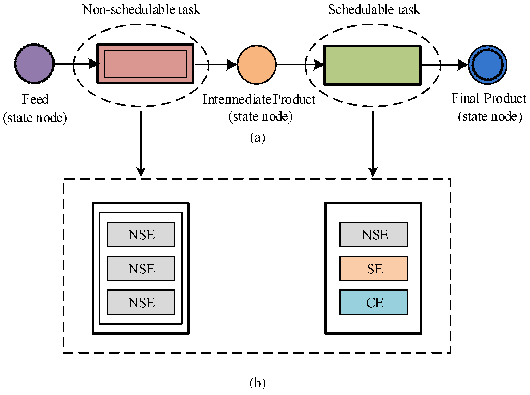
Figure 1a, the DR scheme has state nodes including feed, intermediate product and final product, and task nodes which can be subdivided into non-schedulable tasks (NSTs), for which the electricity demand cannot be scheduled and must be satisfied immediately (for technical or economic reasons); and schedulable tasks (STs), for which the electricity demand can be scheduled among pre-specified multiple operating points.
Figure 1b shows the simple internal structure of each task with the corresponding industrial equipment. In this DR scheme, the industrial equipment is classified into three types: non-shiftable equipment (NSE), which should have a sufficient supply of electricity whenever it is required; shiftable equipment (SE), which can be switched on or off to balance the electricity supply; and controllable equipment (CE), which has multiple operating states with different electricity demands. Based on the properties of each type of equipment, NSTs will be only composed of NSEs, and STs can consist of one or more NES, SE, or CE pieces.
The specific algorithm for the DR scheme is formulated using MILP, which consists of one objective function defined to minimize the energy cost of manufacturing processes, and a series of linear constraints that ensure achievement of the objective without degrading the production line. Constraints are specified for the process modeling (including operating constraints and material balance) and ESS modeling. Once the MILP problem is solved, the outputs of the DR algorithm include the optimal operating point for all STs in each time interval, the charging/discharging rate of ESS in each time interval, the amount of electricity purchased from the grid, and the total energy costs of manufacturing process.
4. Modeling of Automobile Manufacturing
Based on the description of an automobile production line given in [
29], an STN model for DR in automobile manufacturing was developed as shown in
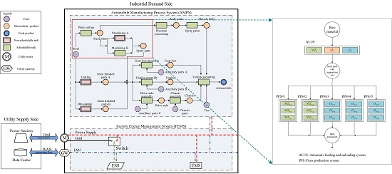
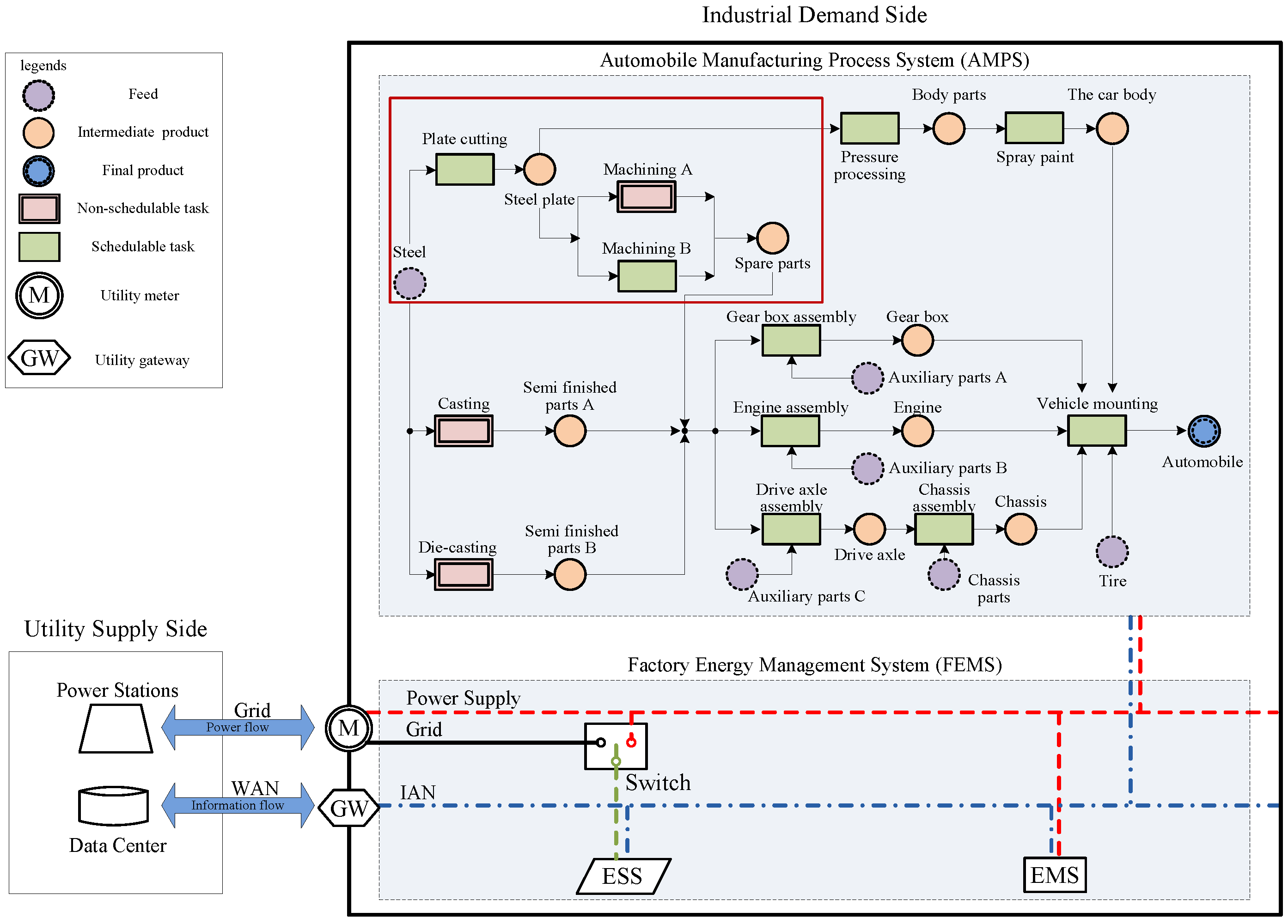
Figure 2. With the utility meter and utility gateway as boundaries, the DR model is composed of a utility supply side and an industrial demand side. The utility meter measures total electricity supplied to the industrial demand side, and the utility gateway exchanges information between a wide area network (WAN) and an industrial area network (IAN).
The utility supply side includes power stations to provide electrical energy for industrial manufacturing through the electrical grid, and a utility data center to communicate with the industrial demand side via the WAN. The industrial demand side is also composed of two subsystems, the automobile manufacturing process system (AMPS) which includes the whole automobile production process represented by the STN model, and the FEMS which includes an energy management system (EMS), ESS, the power source switch, the power supply network, and the IAN.
The AMPS consists of 17 state nodes that include six kinds of feeds represented as broken circles, 10 kinds of intermediate products represented as solid circles, and one final product represented as an inside-broken and outside-solid circle. Additionally, 12 task nodes include three NSTs represented as double-bordered rectangles and nine STs represented as single-bordered rectangles.
In the FEMS, the EMS manages and monitors the electricity demand of the whole automobile manufacturing process. It communicates with the utility supplier via the WAN to obtain day-ahead hourly electricity prices and transmit energy consumption information. Additionally, it schedules STs to work on the optimal operating points to manage the electricity demand of the whole industrial manufacturing, through which parts of the electricity demand can be shifted from peak to off-peak demand periods. By controlling the power source switch, the EMS schedules the ESS to charge electricity from the electrical grid during off-peak periods, or discharge to supply energy for the automobile manufacturing process during peak periods.
In the whole automobile manufacturing, the stamping process emphasized by a red rectangle in
Figure 2, was selected as an example for precise analysis, since it not only determines the quantities of final production but also relates critically to the steady production of subsequent processes through providing sufficient materials for them. Based on the significant feature of discrete manufacturing whereby each process deployed in the discrete manufacturing can be started or stopped individually with a variety of production rates [
30], separate processes shown in
Figure 2 can be combined in a parallel or serial way to expand the scale of the production. Hereon, this study focuses on the stamping process to represent DR management in automobile manufacturing; however, this approach and results can be expanded to the whole process of automobile manufacturing. Applying a DR energy management scheme to the stamping process reduces the energy costs of industrial manufacturing without degrading production processes.
4.1. The Demand Response Representation for the Stamping Process
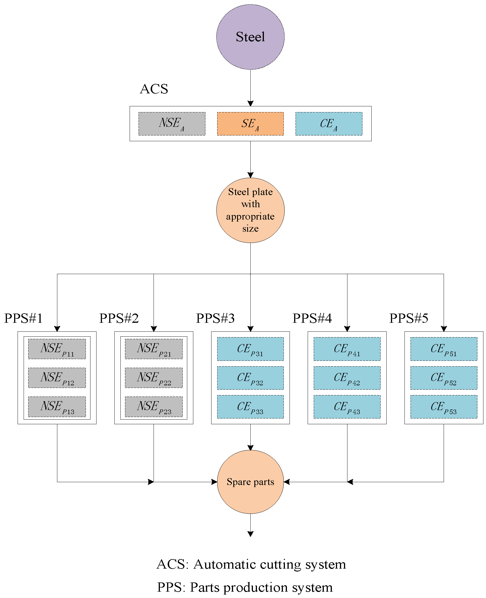
Figure 3 shows the DR representation for the stamping process, which incorporates production processes from steel (raw material) to spare parts (intermediate products of the whole production line). The stamping process can be regarded as two subsystems: the automatic cutting system (ACS) corresponding to plate cutting task in
Figure 2, and the parts production system (PPS) corresponding to machining A task or machining B task in
Figure 2.
The ACS is an ST and consists of three pieces of industrial equipment, which are classified as NSE, SE and CE, respectively. PPS#1 and 2 (both of which correspond to the machining A task) are NSTs and consist of three pieces of industrial equipment regarded as NSEs. PPS#3, 4, and 5 (each of which corresponds to the machining B task) are STs and consist of three pieces of industrial equipment regarded as CEs.
4.2. The Internal Structure of Each Task in the Stamping Process
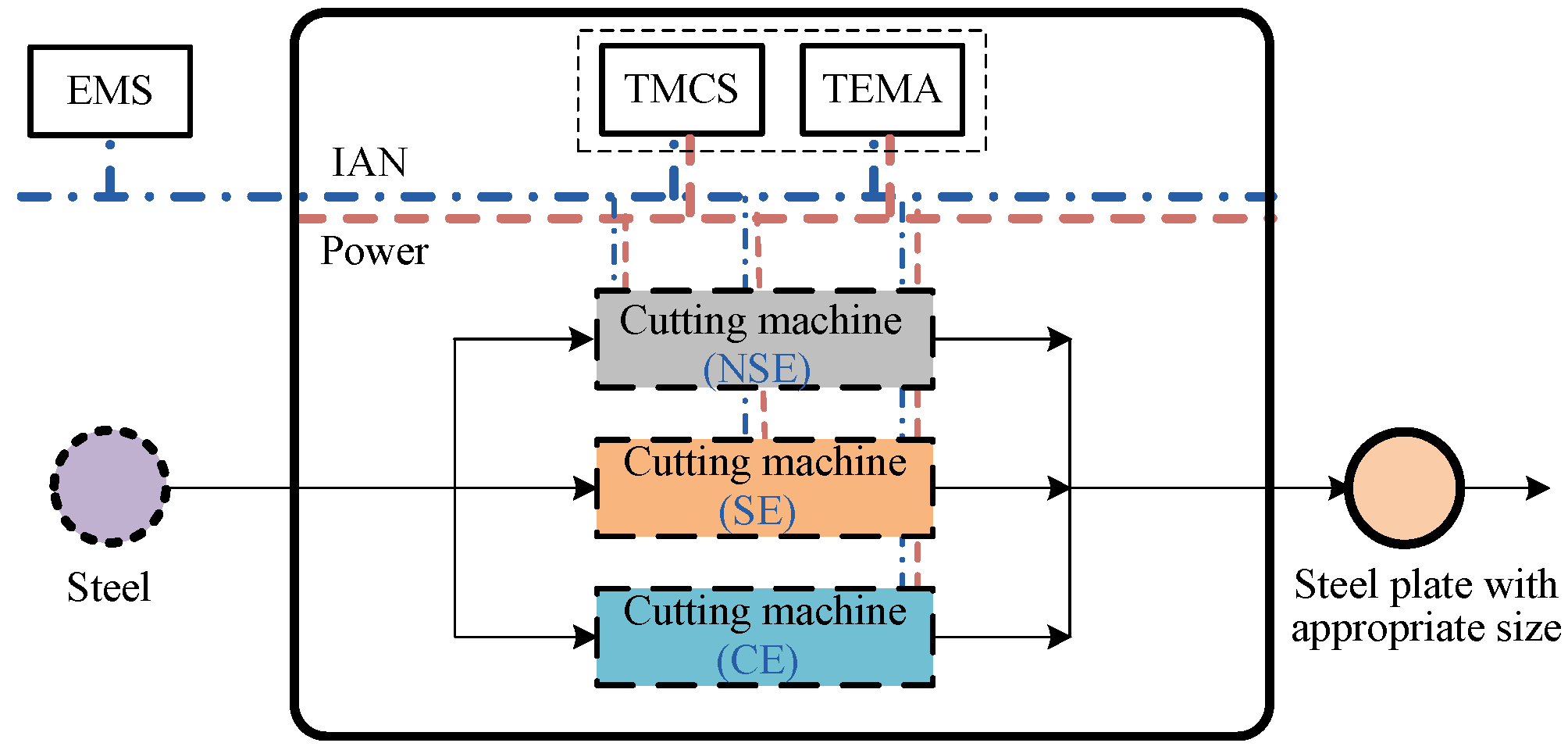
Figure 4 shows the internal structure of the ACS task, which consists of a local task monitoring and control system (TMCS), a local task energy management agent (TEMA), and three pieces of industrial equipment—the different types of cutting machine.
The TMCS monitors and controls the operational state of each piece of equipment in that task. The TEMA monitors electricity consumption and controls the electric load of that task, while exchanging information with the EMS through IAN.
The information exchanged from TEMA to EMS includes the type of each task (NST or ST), the operating points of the task and the current storages of related states. While the operating point itself contains the information of the consumption rate of states (feed or/and intermediate product), the production rate of states (intermediate product or/and final product), and the corresponding electricity demand of the task.
In the ACS task, these cutting machines cut the steel into steel plate with several appropriate sizes, which will be used as materials for other tasks. The ACS is assumed to have three kinds of cutting machines corresponding to NSE, SE and CE, respectively. The first type (which may be a general-purpose machine tool) regarded as an NSE, has only one operating state since it has a long start-up time and cannot be stopped arbitrarily once launched. The second type (which may be a high-speed precision numerical control machine tool with a fixed strokes per minute) regarded as an SE, has two work states (on or off) since it can be started or stopped immediately. The third type (which may be a high-speed precision numerical control machine tool with a variable strokes per minute) regarded as a CE, which has multiple operating states with different consumption rates of materials, generation rates of products, and corresponding electricity demands, since it can be changed from one working state to another in a short time. By managing the operating states of SE and CE, the TEMA defines multiple operating points for the ACS task and reports the current state of each operating point to the EMS through the IAN. The operating point with a low production rate consumes electrical energy at a low rate, while the operating point with a high production rate consumes electrical energy at a high rate. Based on the dynamic day-ahead electricity prices from the utility supply side, the EMS makes optimal decisions on operating points for each task during each time interval, and then transmits this information to the TEMA. According to the information from the TEMA, the TMCS controls each piece of equipment to work on the corresponding operating state. The TEMA then transmits consumption data collected from each piece of equipment to the EMS through the IAN. As shown in
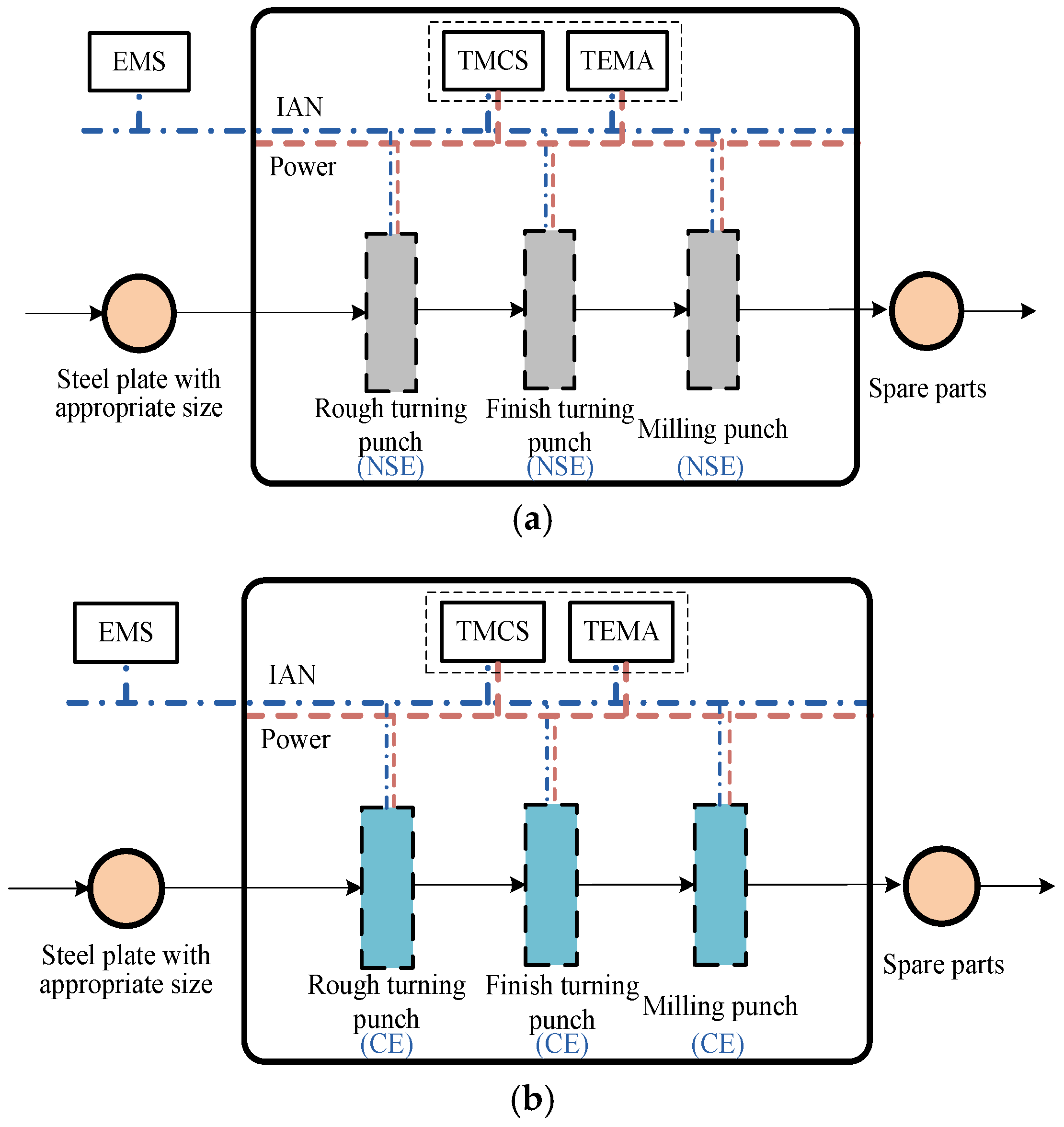
Figure 5, the internal structure of each PPS task has a local TMCS, a local TEMA and three pieces of industrial equipment matched with corresponding three steps in the PPS task.
The PPS task basically involves three steps (rough turning, finish turning, and milling processes) to produce spare parts from steel plate. Each step matches with one kind of punch machine. During the rough turning, the steel plate is produced into semi-finished parts with low accuracy. These semi-finished parts can then be precision machined through the finish turning step. After milling, the processed semi-finished parts are used to produce different spare parts with a variety of surfaces, which is the final product of the stamping process.
Figure 5a shows the internal structure of PPS#1 and 2. They are NSTs, and each of them is composed of three pieces of equipment, which are all NSEs matched with the three steps of the PPS task.
Figure 5b shows the internal structure of PPS#3, 4 and 5. They are STs, and each of them is composed of three pieces of equipment, which are all CEs corresponding to the three steps of the PPS task.
5. Demand Response Scheme for Factory Energy Management Systems
This section consists of two subparts to introduce the DR scheme proposed in [
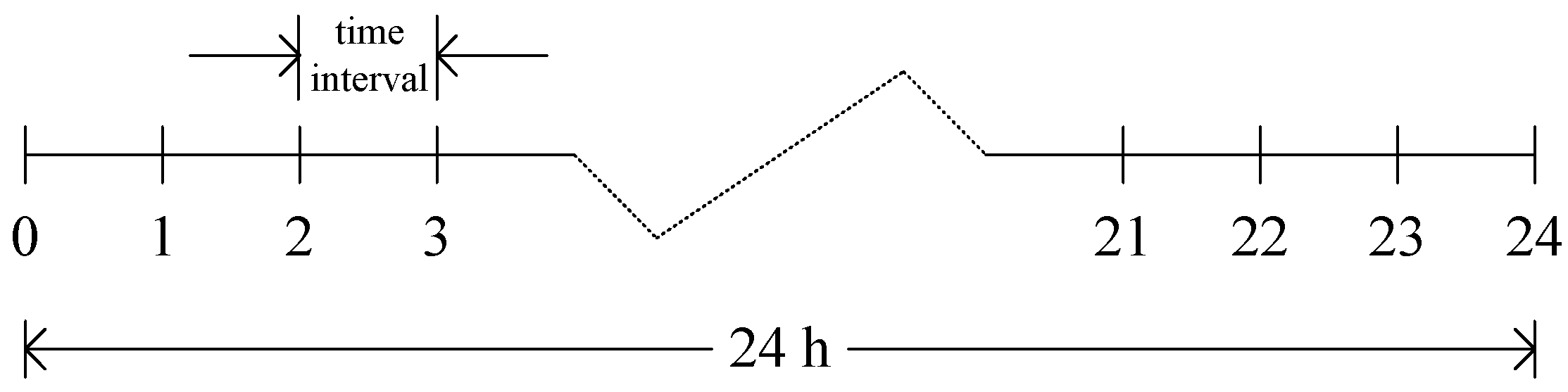
27]. The first one discusses the pure DR scheme (excluding ESS) for an FEMS in SG. The second includes an ESS, which can be integrated into the DR scheme. The DR scheme is operated on the basis of the day-ahead hourly electricity prices, and the time horizon of 24 h is discretized into 24 time intervals with each interval having the same time duration of 1 h, as shown in
Figure 6.
There are some operational scenario requirements for practical application of the DR scheme. First, tasks must take operations (including start operation, end operation, and changes between two different operating points) at the boundaries of time intervals shown in
Figure 6. Second, the electricity demands and related states (i.e., the feed, intermediate product, and final product) of the NSTs and STs during each time interval are assumed to be known a priori at the start of the time horizon.
Based on the inputs (including the day-head hourly electricity prices, the STN model of industrial manufacturing, and the operating information of each task), the DR algorithm selects the optimal operating point for each ST within each pre-specified time interval to efficiently manage energy consumption in the manufacturing process. In other words, DR can schedule STs to work at different operating points through which parts of the electricity demand can be shifted from peak to off-peak periods.
5.1. Demand Response Algorithm
This section describes the optimization problem for the MILP in DR algorithm, which includes the objective function and a series of constraints on processing modeling.
5.1.1. Objective Function
As shown in Equation (1), the objective function is defined as the total energy cost of industrial manufacturing, which should be minimized:
where
pt is the unit electricity price purchased from the utility during time interval (
t,
t + 1), and
Dt is the total electricity demand for the industrial manufacturing process from the electrical grid, which is equal to the summation of the electricity demand for each task within the same time interval,
dk,t. For an NST,
dk,t is fixed during whole time horizon, while for a ST,
dk,t is constrained by operating point, which will be described later.
5.1.2. Constraints on the Process Modeling
Constraints on the processing modeling are subdivided into operating constraints for STs and balance constraints on materials.
Operating Constraints for Schedulable Tasks
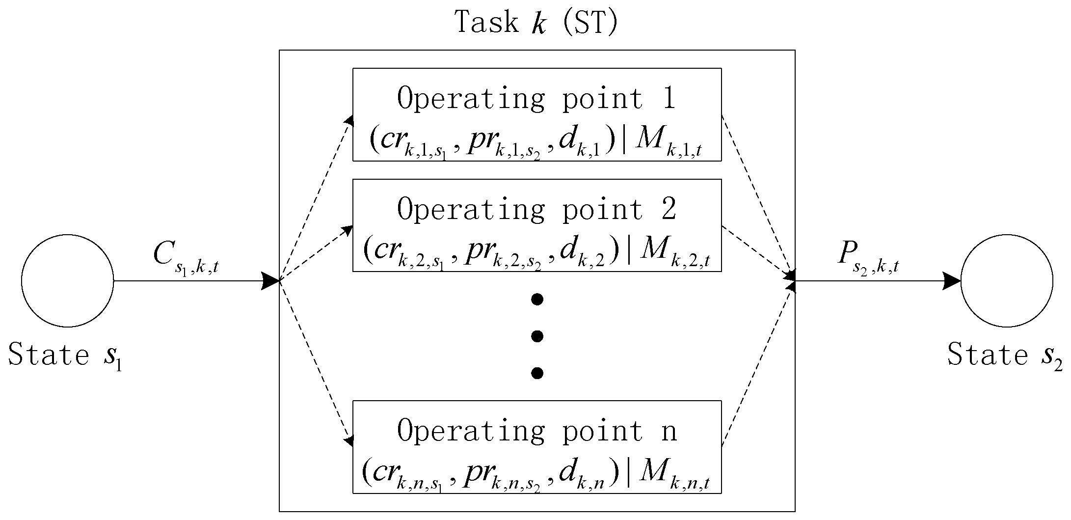
Assuming that task
k is a ST as shown in
Figure 7, it consumes state
s1 to produce state
s2 by choosing one of
n operating points during each time interval. Each operating point is composed of two sets of parameters. The first is a pair of parameters including the consumption rate of raw material
crk,n,s1, generation rate of product
prk,n,s2 and corresponding electricity demand of that task
dk,n. The second is a binary variable
Mk,n,t to indicate if task
k operates at operating point
n during time interval (
t,
t+1) or does not (if the task operates,
Mk,n,t = 1, otherwise
Mk,n,t = 0). Among all operating points (from operating point 1 to operating point
n), Equation (3) restricts that a ST
k must operate at only one operating point within the same time interval.
Figure 7 shows the relation between state s
1 and state s
2 through one ST to indicate the operation mechanism of the ST. In terms of any STs which can consume/produce states, Equations (4)–(6) indicate general relations between states and tasks.
where
Cs,k,t is the quantity of state
s consumed by task
k during time interval (
t,
t + 1).
Ps,k,t is the quantity of state
s produced by task
k within time interval (
t,
t + 1).
dk,t is the electricity demand of task
k during time interval (
t,
t + 1). In Equations (4)–(6), binary variables
Mk,n,t are restricted by Equation (3) to ensure that only one operating point of ST can be operational within the same time interval.
Balance Constraints on Materials
In Equation (7),
SAs,t is the storage of each state
s at time boundary
t (
t > 0), which is equal to the storage at the previous time boundary
t − 1 minus the total amount of state
s consumed within time interval (
t − 1,
t) plus the total amount of state
s produced within time interval (
t − 1,
t):
where
and
are the total amounts of state
s consumed and produced by all task
k (including NSTs and STs) within time interval (
t − 1,
t), respectively. Meanwhile, the storage is typically constrained within fixed limits (
Ssmin,
Ssmax) as shown in Equation (8), which are the lower storage bound and the upper storage bound of each state
s, respectively.
5.2. Demand Response Scheme Integrated with the Energy Storage System
In addition to the processing modeling above, this section integrates an ESS into the previous DR scheme. In this new scheme, the DR also schedules the operation of the ESS during each time interval. For example, during off-peak periods, the DR schedules the ESS to charge energy from the power grid, whereas during peak periods, it schedules the ESS to discharge to supply energy for industrial manufacturing processes. On this basis, the objective function should be modified to include the interaction of the ESS, as well the constraints on ESS modeling need to be taken into account.
5.2.1. Modified Objective Function
With the interaction of ESS, the objective function is modified as Equation (9).
is the total electricity demand of industrial manufacturing from the electrical grid within the interaction of the ESS in time interval (
t,
t + 1), and it is equal to the energy consumption of all tasks
Dt plus the charging energy of the ESS
Ec,t, minus the discharging energy of the ESS
Ed,t:
where
pt and
Dt are as in Equation (1).
5.2.2. Constraints on Energy Storage System Modeling
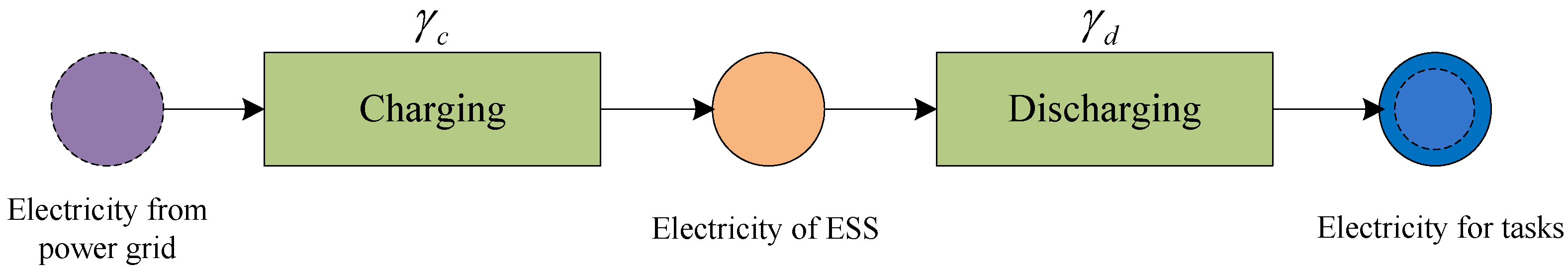
Figure 8 shows the STN model of the ESS, which consists of state nodes including electricity from the power grid, electricity of the ESS, and electricity for tasks; and task nodes including the charging and discharging tasks, both of which are regarded as STs. In order to map the charging and discharging efficiency of the ESS in actual plants, γ
c and γ
d represent charging and discharging coefficients, respectively.
Equation (11) shows the balance relationship of the stored energy in the ESS.
Eess,t is the energy storage at time instant
t, which is equal to the stored energy at previous time instant
t − 1 plus the energy input from charging within time interval (
t − 1,
t) multiplied by the charging efficiency, i.e.,
and minus the energy output from discharging within time interval (
t − 1,
t) divided by the discharging efficiency, i.e.,
.
where
Eess,t is typically constrained within fixed limits (0,
Cess), while
Ec,t and
Ed,t are typically constrained with fixed limits (0, θ
c) and (0, θ
d), respectively. The binary variables
Mc,t and
Md,t indicate whether the ESS is charging or discharging respectively, within time interval (
t,
t + 1).
Mc,t = 1 and
Md,t = 1 indicate that the ESS is charging or discharging respectively, during time interval (
t,
t + 1), otherwise
Mc,t = 0 and
Md,t = 0. Equation (15) restricts that the ESS cannot be both charging and discharging during the same time interval.
6. Results
This section presents the operational scenario and corresponding simulation results of the DR scheme for the stamping process in
Figure 3.
6.1. Operational Scenario
The ACS has five operating points (
Table 1), each of which has related parameters including the cutting frequency of each cutting machine, the parts production amount of the task, and the corresponding electricity demand of the task.
PPS#1 and 2 have only one operating point (
Table 2), with related parameters including the production frequency of each punch machine, the parts production amount of the task, and the corresponding electricity demand of the task. Among those parameters, the production frequency indicated the feed consumption rate and the product generation rate of the corresponding punch machine. For example, the production frequency of
NSEpi1 was 600 pcs/h, meaning that
NSEpi1 consumed 600 pieces of steel plate and produced 600 pieces of spare parts.
PPS#3, 4 and 5 have five operating points (
Table 3), each of which has the related parameters including the production frequency of each punch machine, the parts production amount of the task, and the corresponding electricity demand of the task.
Table 4 lists the related parameters of steel plate and spare parts. The initial storage and storage capacity of steel plate were set to 1200 and 5000, respectively, while the initial storage and storage capacity of spare parts were respectively set to 200 and 3000. In industrial processes, maintaining some margin for reliable production is preferable. Therefore, we set the parameter
SP_
Init to 1200 and the parameter
PP_
Init to 200 (rather than 0). In the whole production process, the consumption of spare parts in every hour was 3000 pieces, and the storage capacity of the feed (the steel) was assumed to be infinite.
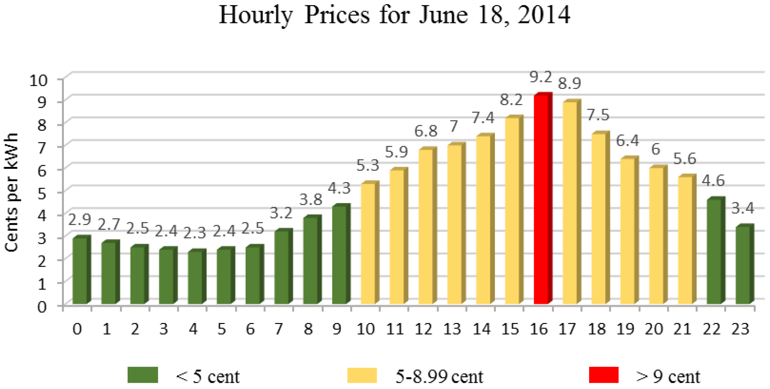
Table 5 lists the parameters related to ESS. The initial storage was 0 kWh and the storage capacity was assumed to be 300 kWh. The maximum charging/discharging rate was set to 75 kWh, and the charging/discharging efficiency coefficient was set to 0.9. The rate of electricity charged/discharged during a given time interval was assumed to be continuously controlled between zero and the maximum charge/discharge rate. Electricity prices were generated using price data obtained from Ameren Illinois Power Company (Belleville, MI, USA) [
31] as day-ahead hourly electricity prices (
Figure 9).
6.2. Optimization Results
Table 6 shows the determined operating points for STs (including ACS and PPS#3, 4 and 5) during each time interval. For example, during time interval 0, the ACS was scheduled to work at operating point 4, so the TMCS of this task controlled the
NSEA to cut steel at a speed of 1200 pieces per hour, the
SEA to be off, and the
CEA to cut steel at a speed of 2100 pieces per hour. During this time interval, this task produced 3300 pieces of steel plate and required 13 kWh of electricity (
Table 1).
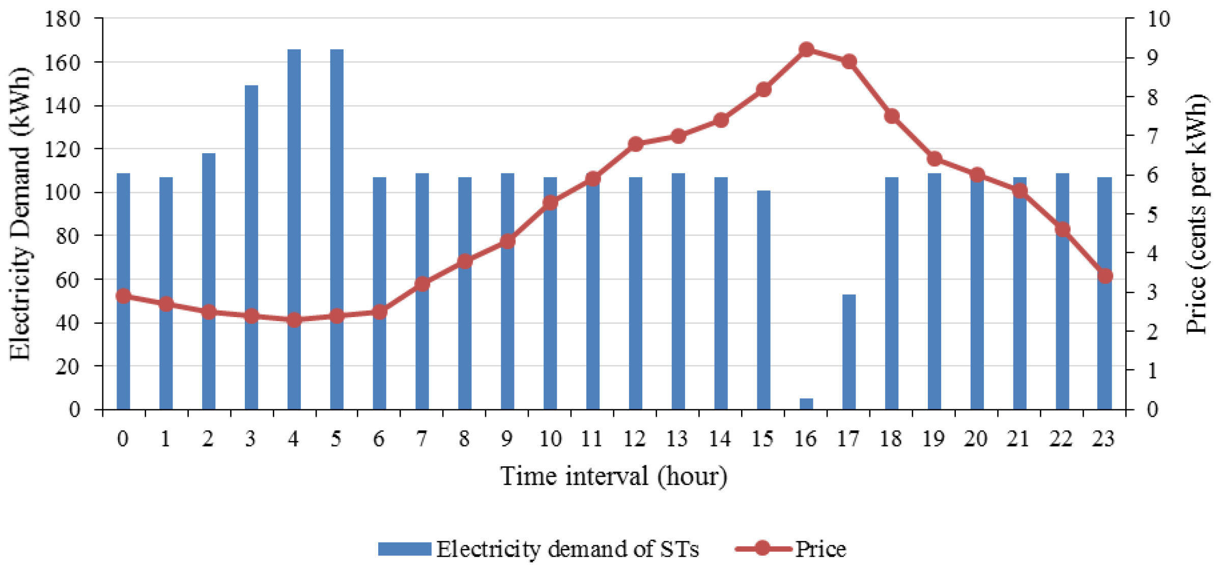
Figure 10 shows the total electricity demand for STs (without interaction of the ESS) during each time interval. According to the dynamic changes in electricity prices, STs (including ACS and PPS#3, 4, and 5) were scheduled to operate at different operating points, as shown in
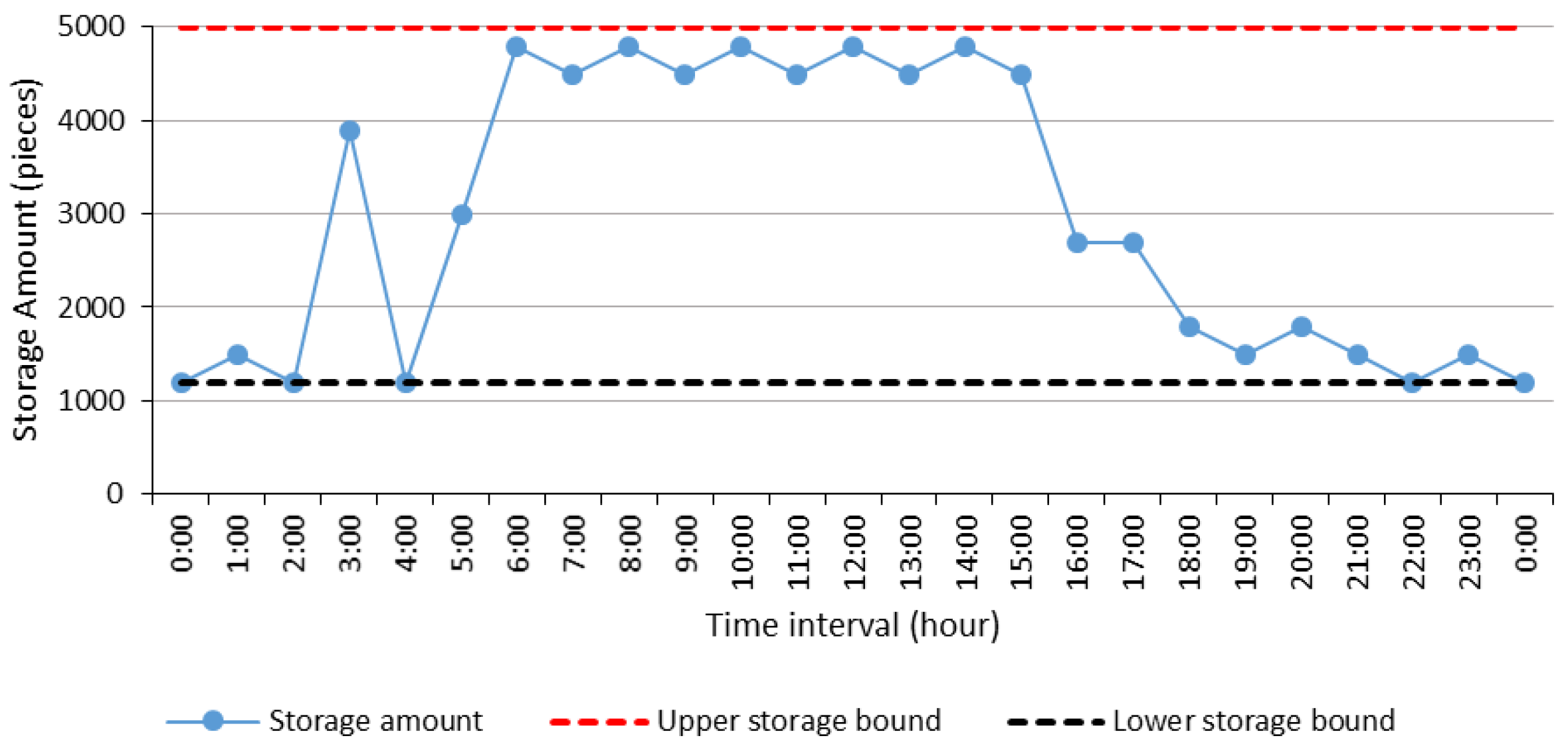
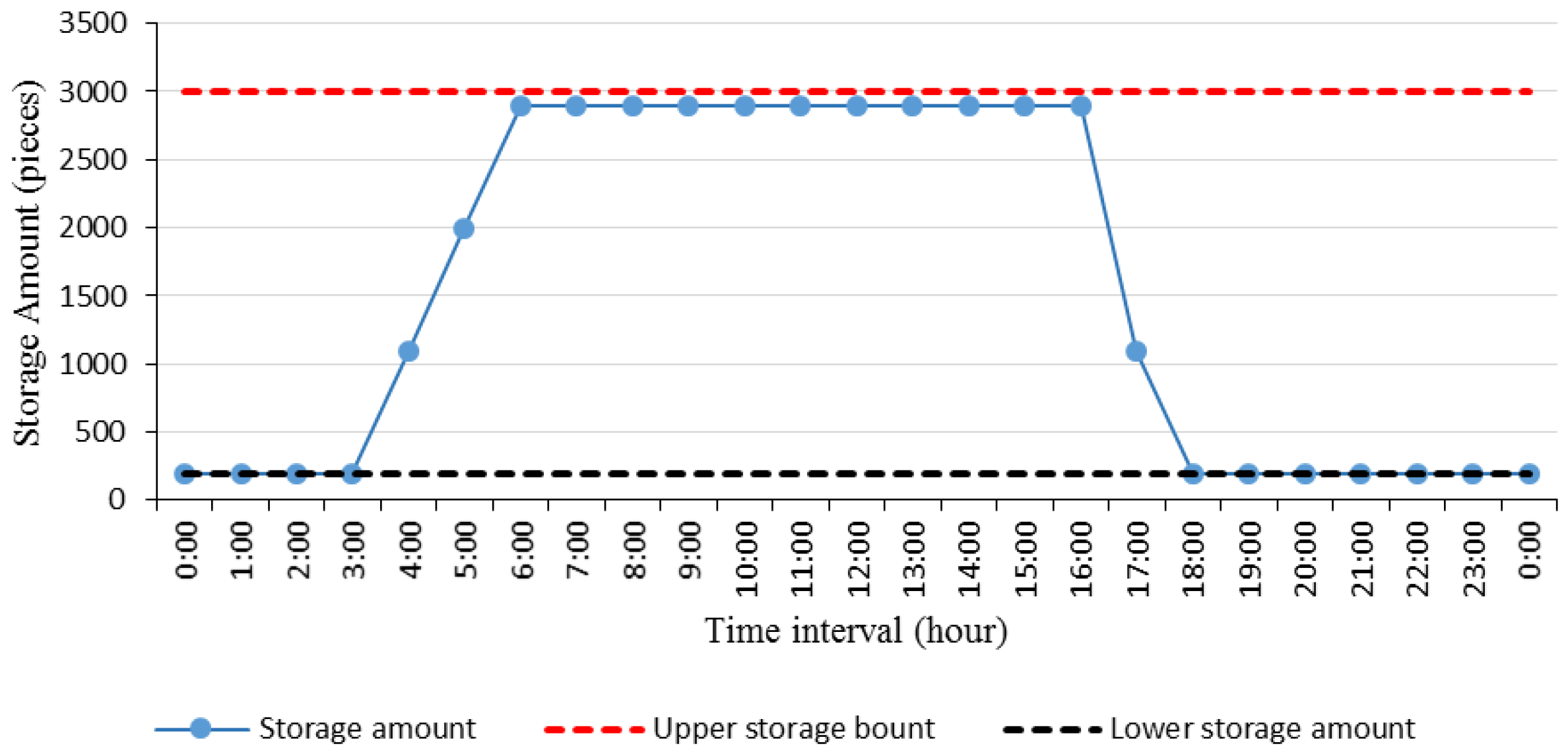
Table 6. When the price was low, STs were scheduled to operate at a high-energy-consumption operating point, increasing electricity demand. Consequently, more steel plate and spare parts were produced and stored during these times, as shown in
Figure 11 and
Figure 12, respectively. When the price was high, STs were scheduled to operate at a low-energy-consumption operating point, decreasing the electricity demand. During these periods, STs produced fewer products, and previously stored products were supplied to subsequent tasks, as shown in
Figure 11 and
Figure 12, which eventually shifted the load from peak to off-peak periods.
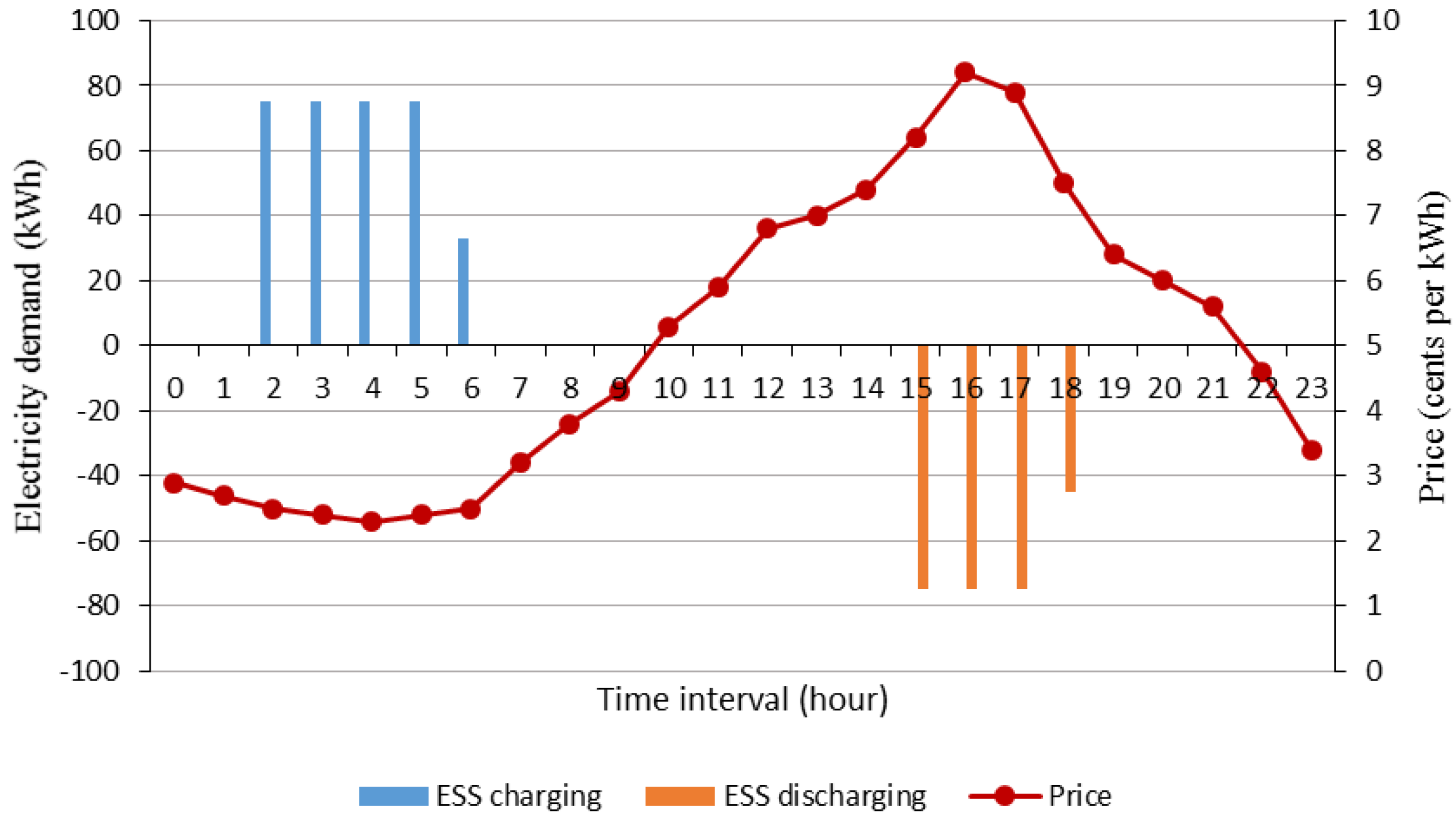
Figure 13 shows the electricity demand of the ESS as a function of the electricity price during each time interval. For electricity demand, positive values indicate charging and negative values indicate discharging. During low-price periods, the ESS charged from the power grid to store energy, while during high-price periods, the ESS discharged to provide electrical energy for industrial manufacturing. During each time interval, the maximum charging/discharging amount of the ESS was 75 kWh, limited by the maximum charging/discharging rate (
Table 5). During time interval 6, the stored energy reached to 300 kWh, which was the storage capacity of the ESS. And the ESS completely discharged all of energy during time interval 18. The total discharged electricity was less than the total charged electricity because of the energy loss during charging and discharging process.
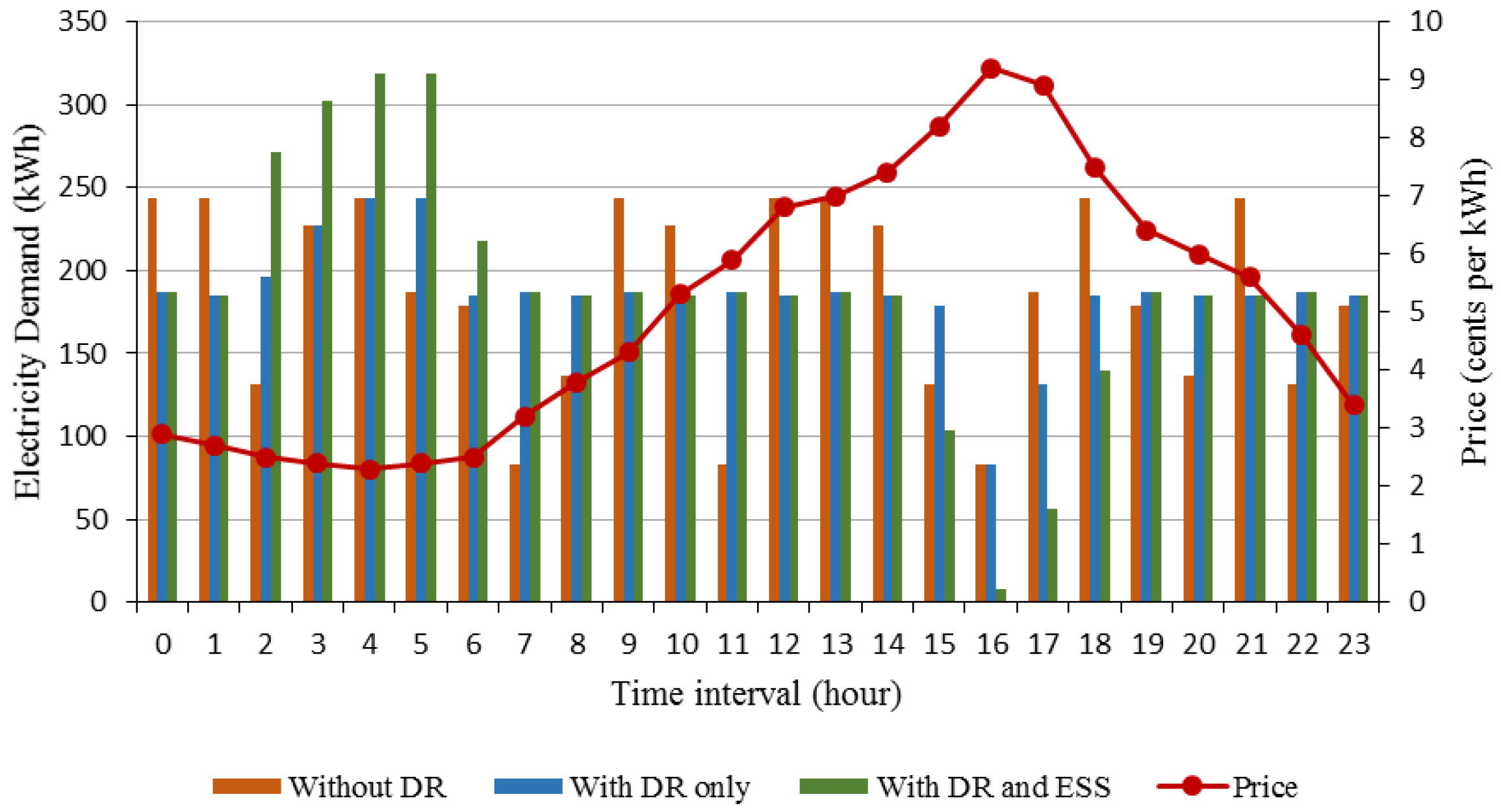
Figure 14 shows the comparison of total electricity demands involving three different test cases. Case a was based on a fixed-price, which was constant over all time intervals and set to be equal to the average of the dynamic price, i.e., no DR function was applied to the FEMS. Case b only considered a DR function based on day-ahead hourly electricity prices. Case c integrated the ESS into the DR function. Compared to Case a, Case b consumed more electrical energy during low-price periods and consumed less electrical energy during high-price periods. In Case c, the energy demand gap between maximum and minimum became larger. Among the three cases, Case c consumed the most electrical energy during low-price periods and consumed the least electrical energy during high-price periods, since the ESS stored energy when prices were low and supplied energy when prices were high. In Case b, the total cost was reduced by shifting demand from high-price periods to low-price periods. In Case c, the total cost was reduced even further not only by shifting demand but also by managing storage through the ESS.
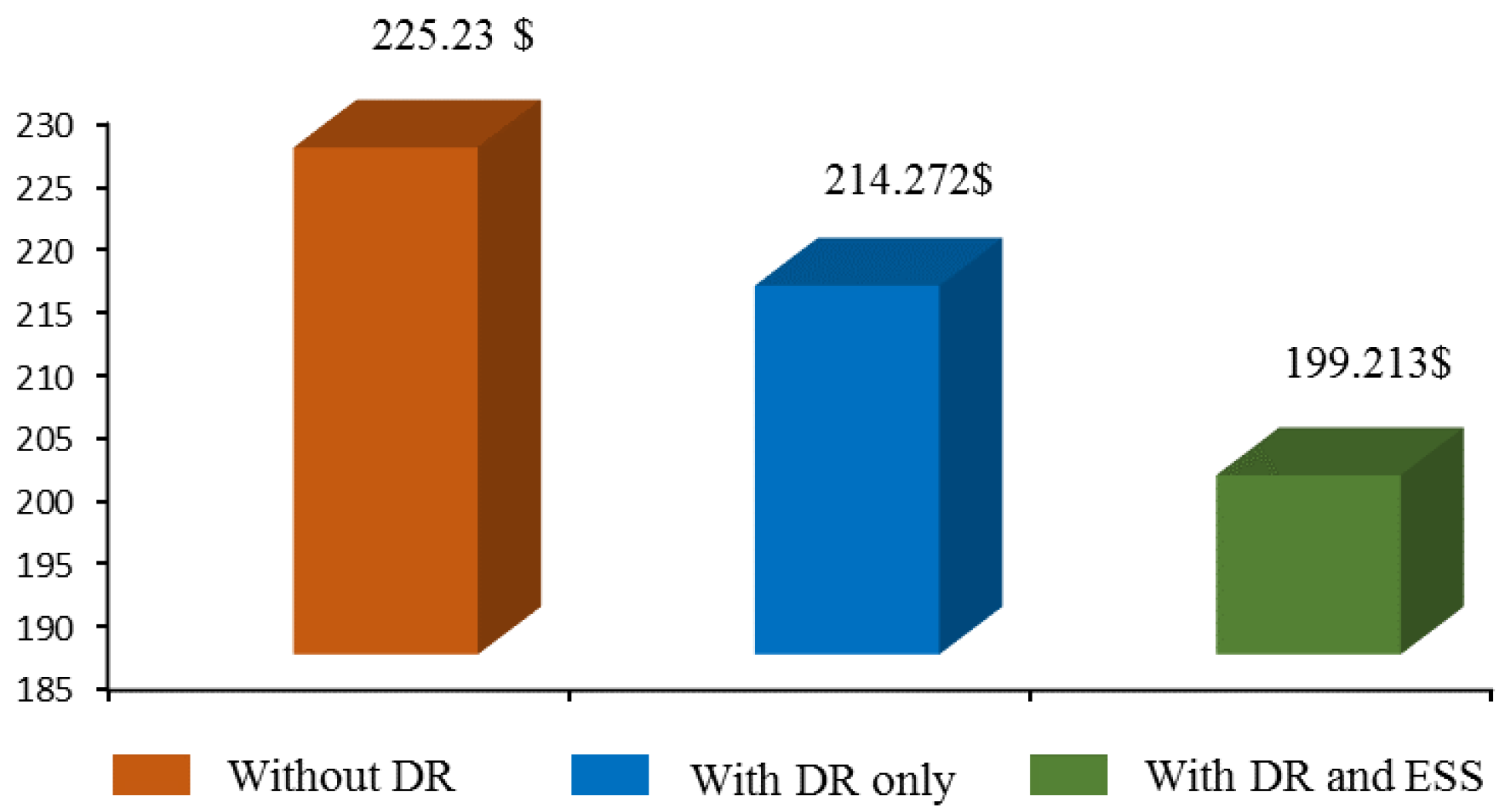
Figure 15 shows a cost comparison for the three test cases in 1 day. The total energy cost for Case c was 11.55% lower than that of Case a.
7. Conclusions and Future Work
As industrial manufacturing becomes more intelligent, many factories have already implemented automatic production systems. Thus, process automation systems have infrastructure for adopting DR-based energy management systems. Against this background, introducing DR into industrial manufacturing has an effective influence on reducing consumption costs. The contributions of this paper are mainly embodied in two aspects, the implementation of a STN representation to a discrete manufacturing system in terms of process operations and energy consumptions, and the application of a DR energy management scheme using the computationally affordable MILP optimization algorithm to discrete manufacturing processes in a SG. The aim of this scheme is to balance energy requirements by shifting electricity demands from peak to off-peak periods and reducing the associated cost. To evaluate the performance of the DR scheme, a typical discrete manufacturing system—automobile manufacturing—was chosen as an example for simulation.
The simulation results showed that when the price was low, STs were scheduled to operate at a high-energy-consumption operating point, increasing electricity demand. Consequently, intermediate products were produced and stored in greater quantities during these periods. When the price was high, STs were scheduled to operate at a low-energy-consumption operating point, decreasing the electricity demand. Less of the corresponding intermediate products were produced and previously stored products were utilized in subsequent tasks during these periods. In contrast, the ESS charged from the power grid to store energy during low-price periods, and discharged to provide energy for industrial manufacturing during high-price periods. Comparing three different test cases: Case a without DR, Case b with DR only, and Case c with DR and ESS, our results indicated that the total costs can be reduced by shifting demand from peak to off-peak demand periods, and reduced further by managing electricity storage through the ESS. Through managing industrial facilities to work at these optimal operating points, the DR scheme provides a significant overall cost reduction without degrading production processes.
In this study, we adopted a simulation model to validate the performance of the proposed DR algorithm. Because the validity of the DR algorithm was verified by the simulation results, one of our future works is to implement the DR algorithm to the actual discrete manufacturing system. Meanwhile, another kind of DERs, the energy generation systems (EGSs) such as solar, wind and waste heat power plants, can be integrated into the DR scheme to further reduce energy costs.


