Optimal Available Transfer Capability Assessment Strategy for Wind Integrated Transmission Systems Considering Uncertainty of Wind Power Probability Distribution

Abstract

Wind power prediction research shows that it is difficult to accurately and effectively estimate the probability distribution (PD) of wind power. When only partial information of the wind power probability distribution function is available, an optimal available transfer capability (ATC) assessment strategy considering the uncertainty on the wind power probability distribution is proposed in this paper. As wind power probability distribution is not accurately given, the proposed strategy can efficiently maximize ATC with the security operation constraints satisfied under any wind power PD function case in the uncertainty set. A distributional robust chance constrained (DRCC) model is developed to describe an optimal ATC assessment problem. To achieve tractability of the DRCC model, the dual optimization, S-lemma and Schur complement are adopted to eliminate the uncertain wind power vector in the DRCC model. According to the characteristics of the problem, the linear matrix inequality (LMI)-based particle swarm optimization (PSO) algorithm is used to solve the DRCC model which contains first and second-order moment information of the wind power. The modified IEEE 30-bus system simulation results show the feasibility and effectiveness of the proposed ATC assessment strategy.

1. Introduction

Wind power energy has become one of the fastest growing renewable energies in recent years. However, the intermittency, randomness and unpredictability of wind power increase the power volatility of the transmission system [1]. With increasing uncertainty in the transmission system, the available transfer capability (ATC) of the transmission system will be influenced greatly. Currently, the wind power prediction accuracy, which to a certain extent has a prediction error, is limited, and it is difficult to obtain the accurate probability distribution function wind power. To improve the security of the transmission system, the wind power uncertainty should be considered in the ATC assessment. Therefore, the probability distribution uncertainty of wind power should be considered to carry out robust and economical ATC assessment strategies [2,3].

In recent years, the research topic of ATC assessment with consideration of wind power uncertainty has seen much activity. The genetic algorithm [4,5], particle swarm optimization [6], optimal power flow method [7], probability analytical method, stochastic programming method [8], Monte Carlo simulation [9,10], and the enumeration method [11] were adopted for this purpose. For describing the wind power uncertainty, the statistical probability method [12,13,14,15] and scene analysis method [16] are adopted. Both of these methods assume that the probability distribution function of wind speed or wind power is determined. In [12], under the determined wind power probability distribution function, the Monte Carlo simulation sampling method is adopted to simulate renewable energy output, and the ATC of transmission system is calculated using optimal power flow under specific grid system status, constraints and parameters. Luo et al. [16] employed the Latin hypercube sampling and scenes cluster analysis to assess ATC with large wind power integration. Shayesteh et al. [17] and Huang et al. [18] assumed that the probability distribution function of wind power is normally distributed. In [18], the ATC assessment problem is described as a kind of chance constrained optimization problem. However, the above proposed statistical probability method and scene analysis method did not consider the uncertainty of the wind power probability distribution function. Due to the fact that the probability distribution function of wind power which is used to describe the uncertainty is also uncertain, the ATC assessment methods mentioned in [12,13,14,15,16,17,18] may be ineffective.

In wind-integrated transmission systems, due to the fact that the wind power prediction technology is limited, adding the geographical complexity, the climate variability and other factors, it is difficult to accurately and effectively estimate the probability distribution function of wind power. Instead, only partial wind power information is available, such as the first and second order moment information [19]. In the prior scenario-based simulation methods and probabilistic analysis methods, wind speeds are assumed to follow a normal distribution [20,21], beta distribution [22,23], Laplace distribution [24,25], Cauchy distribution [26] or other probability distribution functions [27]. However, there is no such uniform probability distribution that is suitable to describe the wind power in all different situations. Based on the available partial information, the exact probability distribution of the wind power even cannot be obtained. Instead, the probability distribution is uncertain and related to a special set of distributions. Therefore, as the above scenario analysis method or probability analytical method do not take this uncertainty into account, they cannot ensure the effectiveness of the ATC assessment strategies.

With the above background, the motivation for this work was to optimize the ATC assessment for wind integrated transmission systems with consideration of all the possible wind power probability distributions. The ATC assessment problem is described as a distributional robust chance constrained (DRCC) model. The dual optimization, Schur complement and S-lemma [28,29] are adopted to eliminate the random variables, and then convert the probabilistic DRCC model into a deterministic model. The linear matrix inequality (LMI)-based particle swarm optimization (PSO) algorithm is used to solve the problem according to its characteristics. This optimization strategy can efficiently maximize the ATC of the transmission system with consideration to all the possible wind power probability distributions with the security operation constraints satisfied. The simulation and analysis of the modified IEEE 30-bus test system verify the feasibility and effectiveness of the proposed strategy.

The rest of this paper is organized as follows: Section 2 introduces the ATC assessment optimization model for wind-integrated transmission systems, which include the chance constrained optimal ATC assessment model and the DRCC optimal ATC assessment model. The solving method for DRCC optimal ATC assessment model, which includes the reformulation of distributional robust chance constraints, the modeling for branch power and node voltage constraints and the determination model for DRCC, is presented in Section 3. Section 4 gives the LMI-based PSO algorithm for the optimal ATC assessment model. Section 5 provides numerical example and case studies. Finally, conclusions are drawn in Section 6.

2. Optimal Available Transfer Capability (ATC) Assessment Model

2.1. Traditional Chance Constrained Optimal Available Transfer Capability (ATC) Assessment Model

For optimal ATC assessment for wind integrated transmission systems considering the uncertainty on the wind power probability distribution chance constrained programming is employed to avoid the operational scheme being limited by small probability events and satisfy the security constraints of the transmission system. The chance constrained optimal ATC assessment model is as follows: the objective function is to maximize the all tie-line power output between a given interface, say, from area a to area b [29]:

$$ATC=\max {\displaystyle \sum P_{a\to b}}$$

(1)

where P_a→b denotes all tie-line power output from area a to area b.

2.1.1. Active and Reactive Power Balance Constraint

$$P_W+P_G-P_D-S_{IJ}^T{P}_L=0$$

(2)

$$Q_W+Q_c+Q_G-Q_D-S_{IJ}^T{Q}_L=0$$

(3)

where P_W and Q_W denote the active and reactive power output of wind farms, respectively; P_G and Q_G denote the active and reactive power output of conventional generators, respectively; P_D and Q_D denote active and reactive loads, respectively; P_L and Q_L denote the active and reactive power flow, respectively; Q_c indicates the actual capacity of reactive power compensators; S_IJ denotes the node branch incidence matrix, which is defined as:

$$S_{IJ}=\{\begin{array}{l}1\mathrm{if}\mathrm{link}IJ\mathrm{starts}\mathrm{at}\mathrm{node}I\\ -1\mathrm{if}\mathrm{link}IJ\mathrm{ends}\mathrm{at}\mathrm{node}I\\ 0\mathrm{else}\end{array}$$

2.1.2. Conventional Unit Generating Capacity Constraints

$$P_{G,\min }\le P_G\le P_{G,\max }$$

(4)

$$Q_{G,\min }\le Q_G\le Q_{G,\max }$$

(5)

where P_G,max and P_G,min denote the upper and lower active power limits of conventional generation, respectively; Q_G,max and Q_G,min denote the upper and lower reactive power limits of conventional generation, respectively.

2.1.3. Active and Reactive Wind Power Output Constraints

$$0\le P_W\le P_{W,\max }$$

(6)

$$0\le Q_W\le Q_{W,\max }$$

(7)

where P_W,max and Q_W,max represent the maximum active and reactive power output of corresponding wind farms, respectively.

2.1.4. Chance Constraints of Node Voltage

$$P{r}_{\mathsf{\varphi }}\{V_{\min }\le V\le V_{\max }\}\ge \mathsf{\beta }$$

(8)

where V, V_max and V_min represent the actual voltage amplitude, upper limit and lower limit of voltage amplitude, respectively. Pr_φ is the probability under φ, where φ is a placeholder for a probability distribution; β is the confidence level.

2.1.5. Chance Constraints of Branch Power

$$P{r}_{\mathsf{\varphi }}\{\left|P_L\right|\le P_{L,\max }\}\ge \mathsf{\beta }$$

(9)

where P_L,max indicates the upper limit of branch power.

Random variables P_W and Q_W exist in the chance constrained optimal ATC assessment model, thus the node voltage and branch power constraints become complicated. The traditional approach to solve the above chance constraints is to use Boole’s inequality [28] to convert these problems into a single chance-constrained problem. The Monte-Carlo sampling method is adopted under the given probability distribution function. However, this method is only efficient if the wind power probability distribution is defined and comprehensively described.

2.2. Distributional Robust Chance Constrained Model

Due to the fact that the wind speed prediction accuracy is limited, the wind speed fluctuates significantly at different seasons over a year, even during different hours over a day. Besides that, geography and climate influence the wind speed a lot. There is lots of uncertain information about wind power and the decision-makers can not get all the information about the probability distribution of wind power. Instead, partial information on wind power such as the first and second order moments can be collected from the historical data. Denote the active output expectations and covariance matrix of m wind farms are μ = [μ₁,…,μ_m]^T and Γ, respectively. Define $\mathrm{\Xi }=\left\{P_W\in {\mathrm{ℝ}}^m:0\le P_W\le P_{W,\max },Q_W\in {\mathrm{ℝ}}^m:0\le Q_W\le Q_{W,\max }\right\}$. Denote Φ_Ξ(μ, Γ) as the set of all the distributions whose mean and covariance are μ and Γ.

The wind probability distribution function may be any one of set Φ_Ξ(μ, Γ), and the predetermined node voltage and branch power constraints should be satisfied under all possible wind power probability distributions.

Therefore, the distributional robust chance constrained model is adopted to describe the optimal ATC assessment problem. When the probability distribution of random variables is uncertain distributional robust chance constrained programming is an effective way to solve such problems [22].

In the node voltage constraints in Equation (8) and branch power constraint in Equation (9), since the probability distribution of the random vector P_W and Q_W are uncertain, P_W and Q_W can be any possible realization under the set Φ_Ξ(μ, Γ), therefore wind power output influences the node voltage and branch power. Therefore, the infimum is introduced in Equations (8) and (9) in the distributional robust chance constrained model to express that for any possible probability distribution function, branch power and node voltages should satisfy the constraints, which is shown in Equations (10) and (11), where $in{f}_{\mathsf{\varphi }\in {\mathsf{\Phi }}_{\mathrm{\Xi }}\left(\mathsf{\mu },\mathrm{\Gamma }\right)}P{r}_{\mathsf{\varphi }}\left\{A\right\}$ represents the minimum probability of A under all possible probability distributions.

$$in{f}_{\mathsf{\varphi }\in {\mathsf{\Phi }}_{\mathrm{\Xi }}\left(\mathsf{\mu },\mathrm{\Gamma }\right)}P{r}_{\mathsf{\varphi }}\{V_{\min }\le V\le V_{\max }\}\ge \mathsf{\beta }$$

(10)

$$in{f}_{\mathsf{\varphi }\in {\mathsf{\Phi }}_{\mathrm{\Xi }}\left(\mathsf{\mu },\mathrm{\Gamma }\right)}P{r}_{\mathsf{\varphi }}\{\left|P_L\right|\le P_{L,\max }\}\ge \mathsf{\beta }$$

(11)

If the probability distribution of wind power isn’t specified, the optimal ATC assessment programs should meet the pre-set confidence level for node voltage and branch power under any possible probability distribution function of set Φ_Ξ(μ,Γ). The difficulty in solving the model is how to handle constraints in Equations (10) and (11) with system node voltage and branch power constraints satisfied when only first and second moment of wind power PD are given.

3. Solving Method for Distributional Robust Chance Constrained Optimal Available Transfer Capability (ATC) Assessment Model

It is impossible to accurately estimate the wind power probability distribution function in the optimal ATC assessment model as analyzed above. The solving process for distributional robust chance constrained ATC assessment model is as follows: firstly, the wind power vector is separated into active and reactive power balance Equations (2) and (3). Secondly, employing the node voltage and reactive power model [30,31], the branch power constraints and node voltage constraints are expressed as a function of wind power. Thirdly, dual optimization, S-lemma and Schur complement are adopted to eliminate the random variable. Finally, the probabilistic based constraints are converted into deterministic constraints.

3.1. Reformulation of Distributional Robust Chance Constraints

Rewrite the node voltage constraints in Equation (10) as follows:

$$\begin{array}{l}in{f}_{\mathsf{\varphi }\in {\mathsf{\Phi }}_{\mathrm{\Xi }}\left(\mathsf{\mu },\mathrm{\Gamma }\right)}P{r}_{\mathsf{\varphi }}\left\{\left|V-\frac{V_{\max }+V_{\min }}{2}\right|\le \left(\frac{V_{\max }-V_{\min }}{2}\right)\right\}\ge \mathsf{\beta }\\ \iff in{f}_{\mathsf{\varphi }\in {\mathsf{\Phi }}_{\mathrm{\Xi }}\left(\mathsf{\mu },\mathrm{\Gamma }\right)}P{r}_{\mathsf{\varphi }}\left\{\left|\Delta V\right|\le \left(\frac{V_{\max }-V_{\min }}{2}\right)\right\}\ge \mathsf{\beta }\end{array}$$

(12)

Employing the node voltage and reactive power model [31], ΔV = JΔQ, where ΔV is the voltage vector increment, ΔQ is the node reactive power injection increment, J is the contraction of Jacobian matrix V – Q. The Newton-Raphson power flow calculation method is adopted in this paper. The core idea is to gradually linearize the nonlinear equations using the Taylor series expansion method. If the initial value is chosen appropriate, which means the first derivative of the initial value is relatively small in the equation, and the second order and higher order term can be omitted. Here in the equation ΔV = JΔQ, ΔQ is the last correction term which can meet the real value of the power balance equation.

The specific power flow calculation of ΔV = JΔQ is as follows:

(1)

Give the initial value of Q(λ) and V(λ), where λ = 0 at the beginning, it denotes the initial value.

(2)

Substitute Q(λ) and V(λ) into the power balance equation [31] to calculate the correction term ΔV(λ) and ΔQ(λ).

(3)

Iteration stops when ΔV(λ) = JΔQ(λ), otherwise, go to Step (4).

(4)

Use ΔV(λ) and ΔQ(λ) to correct Q(λ) and V(λ), then obtains Q(λ + 1) and V(λ + 1), let λ = λ + 1, go back to Step (2).

Here, $\Delta V=J(Q_W+Q_G-Q_D-S_{IJ}^T{Q}_L)$. Substitute ΔV into the node voltage constraint in Equation (12) and eliminate the random variable. Equation (12) can be reformulated as Equation (13), where Prob₁(Q_G) denotes the maximum probability value which satisfies the node voltage constraint under all possible wind power probability distributions:

$$\begin{array}{l}Pro{b}_1\left(Q_G\right)=in{f}_{\mathsf{\varphi }\in {\mathsf{\Phi }}_{\mathrm{\Xi }}\left(\mathsf{\mu },\mathrm{\Gamma }\right)}P{r}_{\mathsf{\varphi }}\left\{\left|J\left(Q_W+Q_G-Q_D-S_{NL}^T{Q}_L\right)\right|\le \left(\frac{V_{\max }-V_{\min }}{2}\right)\right\}\ge \mathsf{\beta }\\ \iff Pro{b}_1\left(Q_G\right)=in{f}_{\mathsf{\varphi }\in {\mathsf{\Phi }}_{\mathrm{\Xi }}\left(\mathsf{\mu },\mathrm{\Gamma }\right)}P{r}_{\mathsf{\varphi }}\left\{\left|\left[\begin{array}{cc}J& J(Q_G-Q_D-S_{NL}^T{Q}_L)\end{array}\right]\left[\begin{array}{c}{Q}_W\\ 1\end{array}\right]\right|\le \left|\left(\frac{V_{\max }-V_{\min }}{2}\right)\right|\right\}\ge \mathsf{\beta }\end{array}$$

(13)

Let $\left[J J\left(Q_G-Q_D-S_{NL}^T{Q}_L\right)\right]=F_1\left(Q_G\right), z_1={\left[Q_W 1\right]}^T$, rewrite Equation (13) as:

$$Pro{b}_1\left(Q_G\right)=in{f}_{\mathsf{\varphi }\in {\mathsf{\Phi }}_{\mathrm{\Xi }}\left(\mathsf{\mu },\mathrm{\Gamma }\right)}P{r}_{\mathsf{\varphi }}\left\{{\left[F_1(Q_G)z_1\right]}^2\le {\left(\frac{V_{\max }-V_{\min }}{2}\right)}^2\right\}\ge \mathsf{\beta }$$

(14)

Let $\left[\left(T_{IJ}^T\right) \left({\mathrm{T}}_{IJ}^T\right)·\left(P_G-P_D\right)\right]=F_2\left(P_G\right), z_2={\left[P_W 1\right]}^T,$ where $T_{IJ}^T$ is the power transmission distribution coefficient matrix [31]. The active power flow P_L can be formulated as follows [31]:

$$\begin{array}{cc}\hfill P_L& =(T_{IJ}^T)\cdot \left(P_W+P_G-P_D\right)\hfill \\ & =\left[\begin{array}{cc}(T_{IJ}^T)& (T_{IJ}^T)\cdot \left(P_G-P_D\right)\end{array}\right]\cdot \left[\begin{array}{c}{P}_W\\ 1\end{array}\right]\hfill \\ & =F_2(Q_G)z_2\hfill \end{array}$$

(15)

Thus, recall $in{f}_{\mathsf{\varphi }\in {\mathsf{\Phi }}_{\mathrm{\Xi }}\left(\mathsf{\mu },\mathsf{\Gamma }\right)}P{r}_{\mathsf{\varphi }}\left\{A\right\}$, denote Prob₂(P_G) as the maximum probability value which satisfies the branch active power constraint under all possible wind power probability distributions:

$$Pro{b}_2(P_G)=in{f}_{\mathsf{\varphi }\in {\mathsf{\Phi }}_{\mathrm{\Xi }}\left(\mathsf{\mu },\mathrm{\Gamma }\right)}P{r}_{\mathsf{\varphi }}\{{\left[F_2(P_G)z_2\right]}^2\le {\left(P_{L,\max }\right)}^2\}\ge \mathsf{\beta }$$

(16)

3.2. Determination Model for Distributional Robust Chance Constraint

According to the dual theory [20], Prob₁(Q_G) and Prob₂(P_G) in Equations (14) and (16) correspond to the optimal value of sub-optimization problem in Equations (17) and (18), respectively. The detailed derivation is shown in Appendix A:

$$\{\begin{array}{l}Pro{b}_1\left(Q_G\right)=\underset{M_{k1}={M_{k1}}^T\in {\mathrm{ℝ}}^{m+1}}{inf}Tr\left(N\cdot M_{k1}\right)\\ s.t.{z_1}^T{M}_{k1}{z}_1\ge 1,\forall z_1\in \left\{{\left[F_1\left(Q_G\right)z_1\right]}^2\le {\left(\frac{V_{\max }-V_{\min }}{2}\right)}^2\right\}\cap \mathrm{\Xi }\\ {z_1}^T{M}_{k1}{z}_1\ge 0,\forall z_1\in \mathrm{\Xi }\end{array}$$

(17)

$$\{\begin{array}{l}Pro{b}_2\left(P_G\right)=\underset{M_{k2}={M_{k2}}^T\in {\mathrm{ℝ}}^{m+1}}{inf}Tr\left(N\cdot M_{k2}\right)\\ s.t.{z_2}^T{M}_{k2}{z}_2\ge 1,\forall z_2\in \left\{{\left[F_2\left(P_G\right)z_2\right]}^2\le {\left(P_{L,\max }\right)}^2\right\}\cap \mathrm{\Xi }\\ {z_2}^T{M}_{k2}{z}_2\ge 0,\forall z_2\in \mathrm{\Xi }\end{array}$$

(18)

where Tr(·) denotes the trace operations, N = [Γ + μμ^T, μ; μ^T, 1], M_k1 and M_k2 are symmetric matrices containing all the dual variables.

In a similar way, employing the dual optimization, S-lemma and Schur complement [20,21], the random wind power in the optimization model is eliminated [28], and Equations (17) and (18) are converted into linear matrix inequalities as shown in Equations (19) and (20). The detailed derivation is shown in Appendix B:

$$\{\begin{array}{l}Pro{b}_1\left(Q_G\right)=\underset{M_{k1}=M_{k1}^T\in {\mathrm{ℝ}}^{m+1}}{inf}Tr\left(N\cdot M_{k1}\right)\\ \mathrm{s}.\mathrm{t}.{\mathsf{\tau }}_{k1,l_1}\ge 0,l_1=1,\dots ,m\\ {\mathsf{\tau }}_{k2,l_1}\ge 0\\ {\mathsf{\tau }}_{k3,l_1}\ge 0,l_1=1,\dots ,m\\ M_{k1}+{\displaystyle {\sum }_{i=1}^m{\mathsf{\tau }}_{k1,l_1}{W}_{l_1}}\ge 0\\ \left[\begin{array}{cc}{M}_{k1}-diag\left(0_n,1-{\mathsf{\tau }}_{k2,l_1}{\left[\frac{V_{\max }-V_{\min }}{2}\right]}^2\right)+{\displaystyle \sum _{l=1}^m{\mathsf{\tau }}_{k3,l_1}{W}_{l_1}}& {\mathsf{\tau }}_{k2,l_1}{F_1}^T\left(Q_G\right)\\ {\mathsf{\tau }}_{k2,l_1}{F}_1\left(Q_{\mathrm{G}}\right)& {\mathsf{\tau }}_{k2,l_1}\end{array}\right]\ge 0\end{array}$$

(19)

where in matrix $W_{l_1}\in {\mathrm{ℝ}}^{\left(m+1\right)\times \left(m+1\right)}$ the (l₁, l₁)-th element is 1, and the (l₁, m + 1)-th and (m + 1, l₁)-th element is $-Q_{W,\max ,l_1}/2$, the rest of the elements is 0, and there are m wind farms. The maximum reactive power output of the l₁-th wind farms is $Q_{W,\max ,l_1}$.

$$\{\begin{array}{l}Pro{b}_2\left(P_G\right)=\underset{M_{k2}=M_{k2}^T\in {\mathrm{ℝ}}^{m+1}}{inf}Tr\left(N\times M_{k2}\right)\\ \mathrm{s}.\mathrm{t}.{\mathsf{\tau }}_{k1,l_2}\ge 0,l_2=1,\dots ,m\\ {\mathsf{\tau }}_{k2,l_2}\ge 0\\ {\mathsf{\tau }}_{k3,l_2}\ge 0,l_2=1,\dots ,m\\ M_{k2}+{\displaystyle {\sum }_{i=1}^m{\mathsf{\tau }}_{k1,l_2}{W}_{l_2}}\ge 0\\ \left[\begin{array}{cc}{M}_{k2}-diag\left(0_n,1-{\mathsf{\tau }}_{k2,l_2}{\left(P_{L,\max }\right)}^2\right)+{\displaystyle \sum _{l_2=1}^m{\mathsf{\tau }}_{k3,l_2}{W}_{l_2}}& {\mathsf{\tau }}_{k2,l_2}{F_2}^T(P_G)\\ {\mathsf{\tau }}_{k2,l_2}{F}_2(P_G)& {\mathsf{\tau }}_{k2,l_2}\end{array}\right]\ge 0\end{array}$$

(20)

In matrix $W_{l_2}\in {\mathrm{ℝ}}^{\left(m+1\right)\times \left(m+1\right)}$, the (l₂, l₂)-th element is 1, and the (l₂, m + 1)-th and (m + 1, l₂)-th element is $-P_{W,\max ,l_2}/2$, the rest of the elements is 0, and there are m wind farms. The maximum active power output of the l₂-th wind farms is $P_{W,\max ,l_2}$.

Substitute Equations (19) and (20) into the DRCC optimal ATC assessment model (Equations (1)–(7), (10) and (11)) to replace the node voltage constraint in Equation (10) and branch power constraint in Equation (11), the DRCC-ATC deterministic model is shown in the following equation:

$$\begin{array}{l}\max {\displaystyle \sum P_{a\to b}}\\ S.T.\{\begin{array}{l}\underset{M_{k2}=M_{k2}^T\in {\mathrm{ℝ}}^{m+1}}{inf}Tr\left(N\cdot M_{k2}\right)\ge \beta ,\underset{M_{k1}=M_{k1}^T\in {\mathrm{ℝ}}^{m+1}}{inf}Tr\left(N\cdot M_{k1}\right)\ge \beta \\ P_G,Q_G\in R^n:\\ P_{G,\min }\le P_G\le P_{G,\max }\\ Q_{G,\min }\le Q_G\le Q_{G,\max }\\ {\mathsf{\tau }}_{k1,l_1}\ge 0,{\mathsf{\tau }}_{k1,l_2}\ge 0,{\mathsf{\tau }}_{k2,l_1}\ge 0,{\mathsf{\tau }}_{k2,l_2}\ge 0,{\mathsf{\tau }}_{k3,l_1}\ge 0,{\mathsf{\tau }}_{k3,l_2}\ge 0,l_1,l_2=1,\dots ,m\\ M_{k2}+{\displaystyle {\sum }_{i=1}^m{\mathsf{\tau }}_{k1,l,2}{W}_{l_2}}\ge 0,M_{k1}+{\displaystyle {\sum }_{i=1}^m{\mathsf{\tau }}_{k1,l_1}{W}_{l_1}}\ge 0\\ \left[\begin{array}{cc}{M}_{k1}-diag\left(0_n,1-{\mathsf{\tau }}_{k2,l_1}{\left[\frac{V_{\max }-V_{\min }}{2}\right]}^2\right)+{\displaystyle \sum _{l_1=1}^m{\mathsf{\tau }}_{k3,l_1}{W}_{l_1}}& {\mathsf{\tau }}_{k2,l_1}{F_1}^T(Q_G)\\ {\mathsf{\tau }}_{k2,l_1}{F}_1(Q_G)& {\mathsf{\tau }}_{k2,l_1}\end{array}\right]\ge 0\\ \left[\begin{array}{cc}{M}_{k2}-diag\left(0_n,1-{\mathsf{\tau }}_{k2,l_2}{\left(P_{L,\max }\right)}^2\right)+{\displaystyle \sum _{l_2=1}^m{\mathsf{\tau }}_{k3,l_2}{W}_{l_2}}& {\mathsf{\tau }}_{k2,l_2}{F_2}^T(P_G)\\ {\mathsf{\tau }}_{k2,l_2}{F}_2(P_G)& {\mathsf{\tau }}_{k2,l_2}\end{array}\right]\ge 0\end{array}\end{array}$$

(21)

After the above derivations, it is obvious that the wind power P_W and Q_W do not exist in the optimization problem in Equation (21), and only the first and second moment information of the wind power probability distribution function is needed.

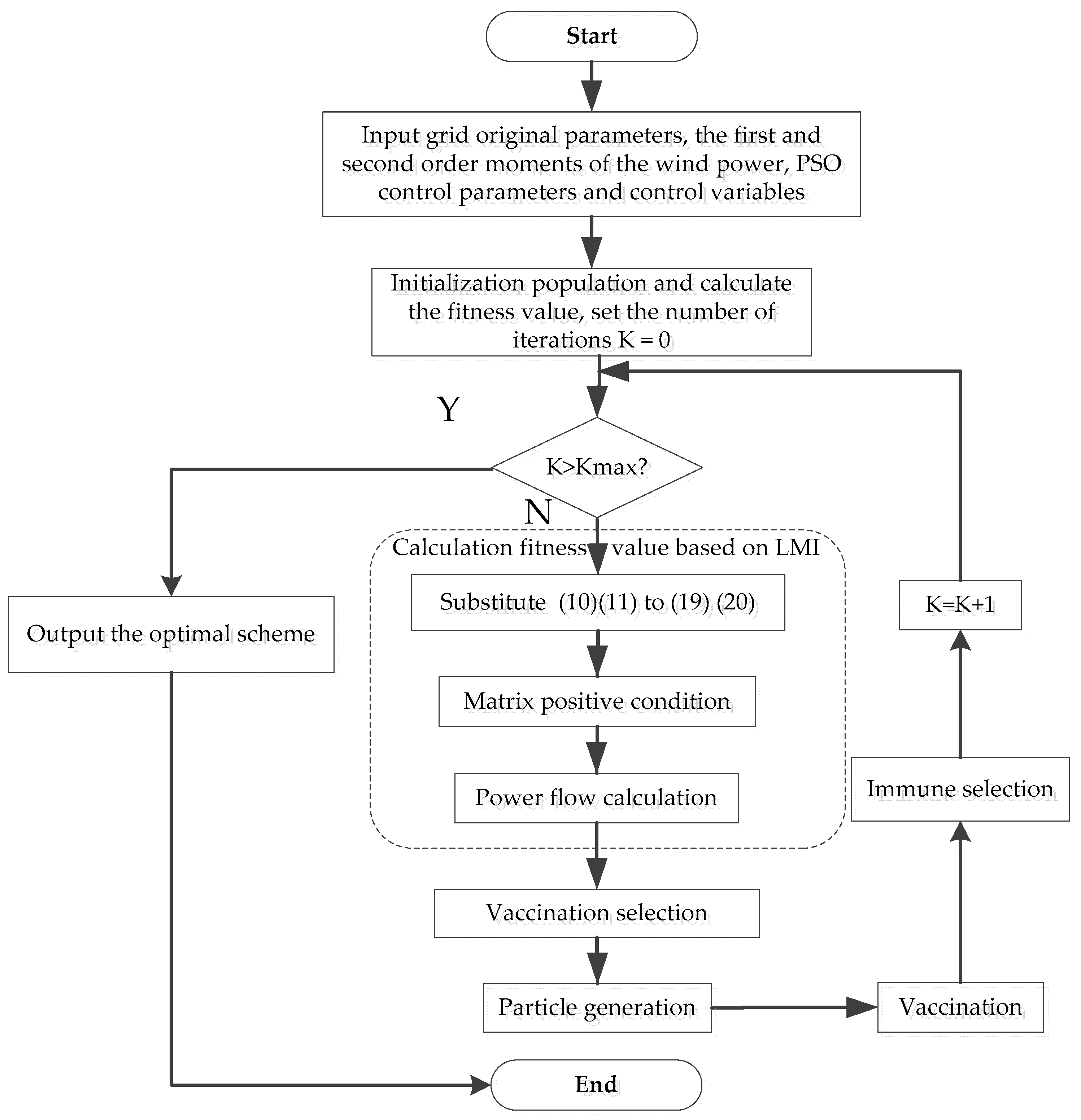
4. Linear Matrix Inequality (LMI)-Based Particle Swarm Optimization (PSO) Algorithm for Available Transfer Capability (ATC) Assessment Problem

The optimal ATC assessment in Equation (21) only needs the first and second order moments of the wind power probability distribution information. It is relatively difficult to solve the nonlinear problem as it includes LMI and nonlinear constraints. The PSO algorithm [32] is used in this paper to solve the problem in Equation (21).

Particle swarm optimization was first proposed by Eberhart and Kennedy. The design of the PSO algorithm is as follows: initialize a group of random particles, each particle represents a candidate solution. The particles update themselves through tracking the personal best position and the optimal solution for the entire population called global minimum, the position of the best particle that give the best fitness value in the entire population. The PSO algorithm has a clear searching direction and it converges quickly at the beginning, however, the PSO algorithm can easily fall into local minimum of convergence speed and precision during the course of evolution. Thus we combine the immune algorithm and PSO, which is expected to address the convergence speed shortcomings of the local minimum of the PSO.

In the PSO updating process, the particles which have high fitness value will be retained. However, if such particles are too concentrated, it can easily to fall into a local optimum. Those particles which have lower fitness value but maintain good evolutionary trends will not be eliminated, so the vaccination strategy based on the diversity of concentration mechanism can efficiently ensure all fitness levels by maintaining a certain concentration, the i-th concentration value of particles is defined as follows:

$$D(x_i)=\frac{1}{{\displaystyle \sum _{j=1}^{num}\left|f(x_i)-f(x_j)\right|}},i=1,2,\dots ,num$$

(22)

where x_i and f(x_i), i = 1,2,…,num, refer to the i-th particle and the fitness value of the i-th particle, respectively. num refers to particle number.

The probability of the particle concentration is defined as follows:

$$Prob(x_i)=\frac{\frac{1}{D(x_i)}}{{\displaystyle \sum _{i=1}^{num}\frac{1}{D(x_i)}}}=\frac{\frac{1}{{\displaystyle \sum _{j=1}^{num}\left|f(x_i)-f(x_j)\right|}}}{\frac{1}{{\displaystyle \sum _{i=1}^{num}{\displaystyle \sum _{j=1}^{num}\left|f(x_i)-f(x_j)\right|}}}},i=1,2,\dots ,num$$

(23)

We can see from the above equation that, if particle j is similar to particle i, then Prob(x_i) is less, which means the chance of particle i to be chosen is less. If the particle j is more different from particle i, then Prob(x_i) is larger. Therefore, the particles have higher diversity.

Immune selection is inspired by the biological immune system. The biological immune system is an intricate network of specialized tissues, organs, cells, and chemicals with the capability of distinguishing entities within the body as “self” or “non-self” and eliminating those that are non-self. If the fitness value of particles is inferior to those of their parent, then the vaccination process is canceled, otherwise, the particles are retained.

The specific flow chart for the LMI-based PSO algorithm for ATC assessment is shown in Figure 1. The specific procedures are as follows:

(1)

Input grid original parameters, the first and second order moments of the wind power, PSO control parameters and control variables. The branch power and node voltage constraints in Equations (10) and (11) can be converted into LMI form as shown in Equations (19) and (20).

(2)

Initialization: set the initial solution $P_G^0$ and $Q_G^0$, calculate the fitness value, and let the iteration counter K = 0.

(3)

Parameter optimization: substitute $P_G=P_G^K$ and $Q_G=Q_G^K$ into sub-problems in Equations (19) and (20). Solve the resulting LMI problem and obtain the optimal solution ${\mathsf{\tau }}_{k1,l_2}^{*} {\mathsf{\tau }}_{k2,l_2}^{*} {\mathsf{\tau }}_{k3,l_2}^{*}$, and set ${\mathsf{\tau }}_{k1,l_2}^K={\mathsf{\tau }}_{k1,l_2}^{*}, {\mathsf{\tau }}_{k2,l_2}^K={\mathsf{\tau }}_{k2,l_2}^{*}, {\mathsf{\tau }}_{k3,l_2}^K={\mathsf{\tau }}_{k3,l_2}^{*}$.

(4)

Optimal decision: substitute ${\mathsf{\tau }}_{k1,l_2}={\mathsf{\tau }}_{k1,l_2}^K, {\mathsf{\tau }}_{k2,l_2}={\mathsf{\tau }}_{k2,l_2}^K, {\mathsf{\tau }}_{k3,l_2}={\mathsf{\tau }}_{k3,l_2}^K$ into Equation (21), solve the matrix positive condition and power flow calculation to obtain the updated optimal solution $P_G^{*}$ and $Q_G^{*}$ and the corresponding objective value $\sum P_{a\to b}^{*}$. Vaccine selection and immune selection are defined as shown in Equations (22) and (23), the particle P_Gi, Q_G,i with high Prob(P_Gi, Q_G,i) value would be selected, and set $P_G^{K+1}=P_G^{*}$ and $Q_G^{K+1}=Q_G^{*}, \sum P_{a\to b}^{K+1}=\sum P_{a\to b}^{*}.$

(5)

Termination: If the iteration counter K meets the predefined value, then the final optima $P_G^{K+1}, Q_G^{K+1} and \sum P_{a\to b}^{K+1}$ are obtained, and the algorithm ends. Otherwise, let K = K + 1, and repeat Steps (3) and (4).

5. Numerical Example

The modified IEEE 30-bus transmission system used for simulation calculation is shown in Figure 2. It is divided into three regions, and the revised system includes six conventional generators, the specific parameters of which are shown in

Table 1. Generator parameters and limits.

Node	1	2	5	8	11	13
PG,max (MW)	139	58	35	21	18	10
PG,min (MW)	130	32	30	13	17	10

. There are 22 P-Q buses (where bus 11 and bus 24 are reactive power compensation points, the compensation step is 0.048), one balance bus (bus 1), and the rest are P-V buses. Upper and lower limits of node voltage are 1.1 pu (per unit) and 0.95 pu. There are 41 branches in the transmission system. The transformer parameters are shown in

Table 2. Transformer parameters and limits.

Branch No.	Tmax	Tmin	Tap Ratio	Unit Capacity
11	1.1	0.9	17	0.0125
12	1.1	0.9	17	0.0125
15	1.1	0.9	17	0.0125
36	1.1	0.9	17	0.0125

. There are six wind farms integrated to the transmission system, which are connected to the grid at bus 3, 16, 23, 26, 27 and 28.

To illustrate the validity of the proposed strategy, we compare the results of the DRCC optimal ATC assessment (DRCC-ATC) model and the TCC optimal ATC assessment (TCC-ATC) model. Wind power is assumed to follow the normal distribution in the TCC model. In order to analyze the impact of wind power on the optimal ATC assessment, we test the ATC assessment strategy under different confidence levels and covariance values.

5.1. Comparison of the Distributional Robust Chance Constrained ATC (DRCC-ATC) Model and the Traditional Chance Constrained ATC (TCC-ATC) Model

To compare the distributional robust chance constrained ATC (DRCC-ATC) model and the traditional chance constrained ATC (TCC-ATC) model, we set the expectation of wind power probability distribution to 2.0 MW, and the covariance of the wind power probability distribution to 0.4 MW². The optimal values of the DRCC-ATC model and the TCC-ATC model under different confidence levels are shown in Figure 3.

Figure 3 illustrates the effect of the confidence level on the ATC. It is shown in Figure 3 that with increasing confidence level, the ATC obtained by the DRCC and TCC both gradually decrease to satisfy the security constraints caused by the wind power uncertainty. For a given confidence level, the ATC under the DRCC model is smaller than that of the TCC model. In the DRCC model, the node voltages and branch power should meet the constraints at a given confidence level under any given wind power probability distribution. In the TCC model, the node voltage and branch power should meet the constraint at a given confidence level for only one kind of wind power probability distribution. Therefore, the DRCC model argues for a more rigid security constraint for the wind-integrated transmission system, which results in a smaller ATC when this model is employed.

5.2. Available Transfer Capability (ATC) under Different Expectations of Wind Power Probability Distribution, Where Covariance = 0.4 MW²

Figure 4 illustrates the relationship between ATC and the wind power probability distribution expectation. Given the same covariance of wind power PD and confidence level, we compare ATC values under different expectations of wind power probability. We can find in Figure 4 that with the increase of the confidence level, ATC gradually decreases. When the confidence level increases, ATC decreases to avoid breaking the security constraints.

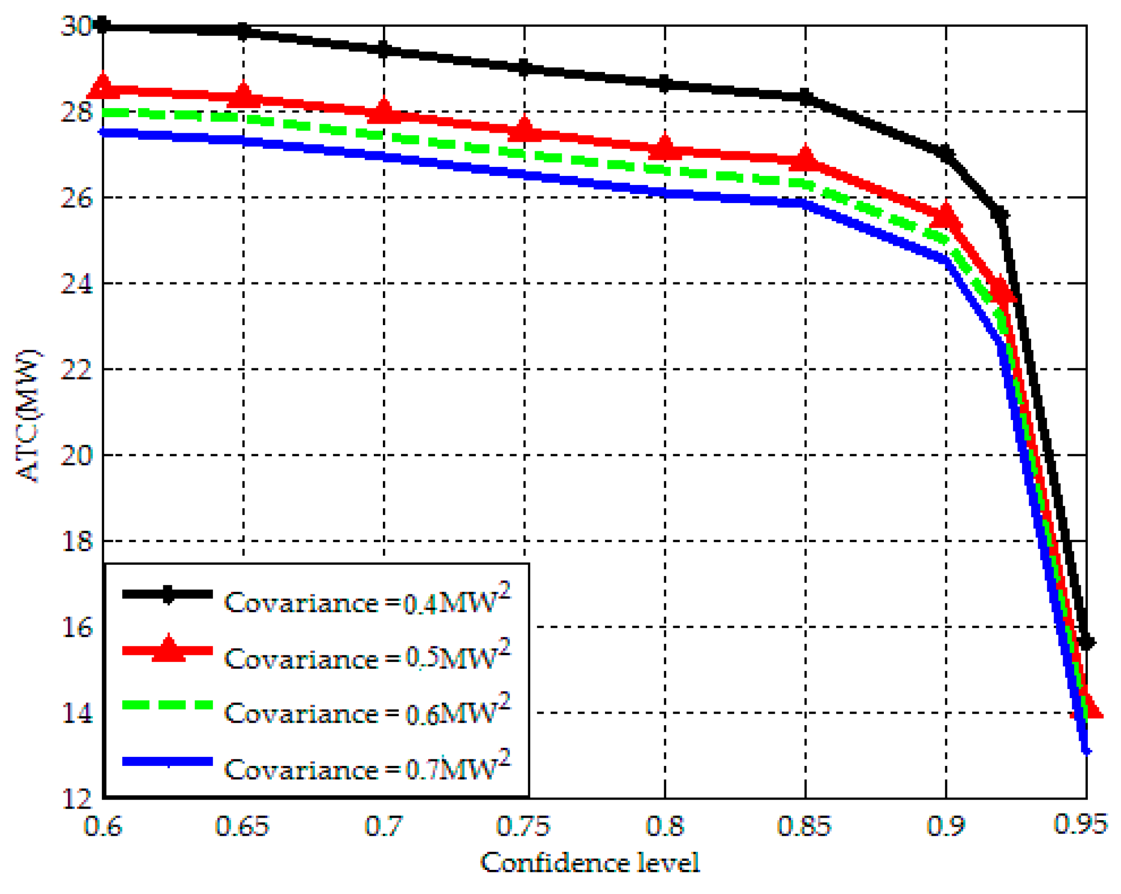
5.3. Available Transfer Capability (ATC) under Different Covariance of Wind Power Probability Distribution, Where Expectation = 2.0 MW

Figure 5 illustrates the relationship between ATC and the covariance of the wind power probability distribution. Given the same expectation of wind power PD and confidence level, we compare ATC under different covariances of wind power probability. We can find that the greater the covariance is, the smaller the corresponding ATC is. If the covariance is greater, which means the fluctuation range of wind power is increased, therefore the branch flow and node voltage change more, which results in an ATC decrease under more strict security constraints.

In the actual wind integrated transmission system operation, the transmission system should set a reasonable confidence level according to the actual situation with the security satisfied to thus obtain an effective ATC assessment scheme.

6. Summary

This paper proposes an ATC evaluation strategy considering the uncertainty on the wind power due to the fact that the exact probability distribution of wind power is not given. With respect to the fact that the partial information such as the first and second order moments of wind power probability distribution can be collected from historical data, a DRCC model is presented for ATC assessment. The proposed method can meet the system requirements for security operation under any possible wind power probability distribution. The DRCC model is converted into a deterministic model. For solving the deterministic model, the PSO algorithm based on the LMI is employed. The effectiveness and feasibility of the proposed optimal ATC evaluation strategy method is verified through numerical examples. In modeling the ATC assessment strategy for a wind integrated transmission system, it is more in accord with the actual engineering situation using the apparent power in the branch power and node voltage model, which we will concentrate on in future research work.

References

1. Thomas, A. Wind Power in Power Systems; John Wiley & Sons: New York, NY, USA, 2005. [Google Scholar]
2. Zhao, P.; Wang, J.; Dai, Y. Capacity allocation of a hybrid energy storage system for power system peak shaving at high wind power penetration level. Renew. Energy 2015, 75, 541–554. [Google Scholar] [CrossRef]
3. Lu, J.; Wei, Z.; Tian, Y. Research on available transfer capability for power system including large-scale wind farms. In Proceedings of the 2011 International Conference on Electrical and Control Engineering (ICECE), Yichang, China, 16–18 September 2011; pp. 2484–2487.
4. Farahmand, H.; Rashidinejad, M.; Mousavi, A.; Gharaveisi, A.A.; Irving, M.R.; Taylor, G.A. Hybrid mutation particle swarm optimization method for available transfer capability enhancement. Int. J. Electr. Power Energy Syst. 2012, 42, 240–249. [Google Scholar] [CrossRef]
5. Liang, D.; Xu, J.; Sun, Z. Research on method of total transfer capacity based on immune genetic algorithm. J. Appl. Sci. Eng. Innov. 2014, 1, 33–38. [Google Scholar]
6. Li, Y.; Wang, B.B.; Wei, Y.L.; Wan, Q.L. Risk Based optimal strategy to split commercial components of available transfer capability by particle swarm optimization method. In Proceedings of the Third International Conference on Electric Utility Deregulation and Restructuring and Power Technologies, Nanjing, China, 6–9 April 2008; pp. 604–609.
7. Xiao, Y.; Song, Y.H.; Sun, Y.Z. A hybrid stochastic approach to available transfer capability evaluation. IEE Proc. Gener. Trans. Distrib. 2001, 148, 420–426. [Google Scholar] [CrossRef]
8. Xu, Y.; Nie, Y.; Liu, W. Predicting available transfer capability for power system with large wind farms based on multivariable linear regression models. In Proceedings of the 2014 IEEE PES Asia-Pacific Power and Energy Engineering Conference (APPEEC), Hong Kong, China, 7–10 December 2014; doi:10. [CrossRef]
9. Othman, M.M.; Busan, S. A novel approach of rescheduling the critical generators for a new available transfer capability determination. IEEE Trans. Power Syst. 2016, 31, 3–17. [Google Scholar] [CrossRef]
10. Chang, R.F.; Tsai, C.Y.; Su, C.L.; Lu, C.N. Method for computing probability distributions of available transfer capability. IEE Proc. Gener. Trans. Distrib. 2002, 149, 427–431. [Google Scholar] [CrossRef]
11. Bofinger, S.; Luig, A.; Beyer, H.G. Qualification of wind power forecasts. In Proceedings of the Global Wind Power Conference, Paris, France, 2–5 April 2002; Volume 1996.
12. Du, P.; Li, W.; Ke, X.; Lu, N.; Ciniglio, O.A.; Colburn, M.; Anderson, P.M. Probabilistic-based available transfer capability assessment considering existing and future wind generation resources. IEEE Trans. Sustain. Energy 2015, 6, 1263–1271. [Google Scholar] [CrossRef]
13. Rodrigues, A.B.; Da Silva, M.G. Probabilistic assessment of available transfer capability based on Monte Carlo method with sequential simulation. IEEE Trans. Power Syst. 2007, 22, 484–492. [Google Scholar] [CrossRef]
14. Stahlhut, J.W.; Heydt, G.T. Stochastic-algebraic calculation of available transfer capability. IEEE Trans. Power Syst. 2007, 22, 616–623. [Google Scholar] [CrossRef]
15. Xiao, Y.; Song, Y.H. Available transfer capability (ATC) evaluation by stochastic programming. IEEE Power Eng. Rev. 2000, 20, 50–52. [Google Scholar] [CrossRef]
16. Luo, G.; Chen, J.; Cai, D.; Shi, D.; Duan, X. Probabilistic assessment of available transfer capability considering spatial correlation in wind power integrated system. IET Gener. Trans. Distrib. 2013, 7, 1527–1535. [Google Scholar]
17. Shayesteh, E.; Hobbs, B.F.; Soder, L.; Amelin, M. ATC-based system reduction for planning power systems with correlated wind and loads. IEEE Trans. Power Syst. 2015, 30, 429–438. [Google Scholar] [CrossRef]
18. Huang, Y.; Wen, F.; Gerard, L.; Xue, Y.; Lei, J. A multi-objective optimization approach for coordinating available transfer capability with risk control. In Proceedings of the 2012 Conference on Power & Energy, Ho Chi Minh City, Vietnam, 12–14 December 2012; pp. 391–396.
19. Bouffard, F.; Galiana, F.D. Stochastic security for operations planning with significant wind power generation. IEEE Trans. Power Syst. 2008, 23, 306–316. [Google Scholar] [CrossRef]
20. Albadi, M.H.; El-Saadany, E.F. Comparative study on impacts of wind profiles on thermal units scheduling costs. IET Renew. Power Gener. 2011, 5, 26–35. [Google Scholar] [CrossRef]
21. Fabbri, A.; Román, T.G.S.; Abbad, J.R.; Quezada, V.H.M. Assessment of the cost associated with wind generation prediction errors in a liberalized electricity market. IEEE Trans. Power Syst. 2005, 20, 1440–1446. [Google Scholar] [CrossRef]
22. Bludszuweit, H.; Dominguez-Navarro, J.A.; Llombart, A. Statistical analysis of wind power forecast error. IEEE Trans. Power Syst. 2008, 23, 983–991. [Google Scholar] [CrossRef]
23. Tewari, S.; Geyer, C.J.; Mohan, N. A statistical model for wind power forecast error and its application to the estimation of penalties in liberalized markets. IEEE Trans. Power Syst. 2011, 26, 2031–2039. [Google Scholar] [CrossRef]
24. Wu, J.; Zhang, B.; Li, H.; Li, Z.; Chen, Y.; Miao, X. Statistical distribution for wind power forecast error and its application to determine optimal size of energy storage system. Int. J. Electr. Power Energy Syst. 2014, 55, 100–107. [Google Scholar] [CrossRef]
25. Hodge, B.M.; Milligan, M. Wind power forecasting error distributions over multiple timescales. In Proceedings of the IEEE Power and Energy Society General Meeting, San Diego, CA, USA, 24–29 July 2011; pp. 24–29.
26. Bian, Q.; Xin, H.; Wang, Z.; Gan, D.; Wong, K.P. Distributionally robust solution to the reserve scheduling problem with partial information of wind power. IEEE Trans. Power Syst. 2014, 30, 2822–2823. [Google Scholar] [CrossRef]
27. Patel, M.; Girgis, A. Review of available transmission capability (ATC) calculation methods. In Proceedings of the Power Systems Conference, Clemson, SC, USA, 10–13 March 2009; pp. 1–9.
28. Yang, W.; Xu, H. Distributionally robust chance constraints for non-linear uncertainties. Math. Program. 2016, 155, 231–165. [Google Scholar] [CrossRef]
29. Zymler, S.; Kuhn, D.; Rustem, B. Distributionally robust joint chance constraints with second-order moment information. Math. Program. 2013, 137, 167–198. [Google Scholar] [CrossRef]
30. Wang, L.; Li, X.R. Robust fast decoupled power flow. IEEE Trans. Power Syst. 2000, 15, 208–215. [Google Scholar] [CrossRef]
31. Gers, J.M. Distribution System Analysis and Automation; The Institution of Engineering and Technology: Hertfordshire, UK, 2013. [Google Scholar]
32. Ren, H.; Zhao, Y. Immune particle swarm optimization of linear frequency modulation in acoustic communication. J. Syst. Eng. Electr. 2015, 26, 450–456. [Google Scholar] [CrossRef]
Figure 1. Flowchart of the linear matrix inequality (LMI)-based particle swarm optimization (PSO) algorithm.
Energies 09 00704 g001
Figure 2. The modified IEEE 30-bus test system.
Energies 09 00704 g002
Figure 3. Optimal ATC obtained by the DRCC and TCC models for the modified IEEE 30-bus system.
Energies 09 00704 g003
Figure 4. ATC under different expectations of wind power PD for the modified IEEE 30-bus system, where the covariance = 0.4 MW2.
Energies 09 00704 g004
Figure 5. ATC under different wind power covariances for the modified IEEE 30-bus system, where expectation = 2.0 MW.
Energies 09 00704 g005