
Annual Atmospheric Corrosion of Carbon Steel Worldwide. An Integration of ISOCORRAG, ICP/UNECE and MICAT Databases


Abstract
:1. Introduction
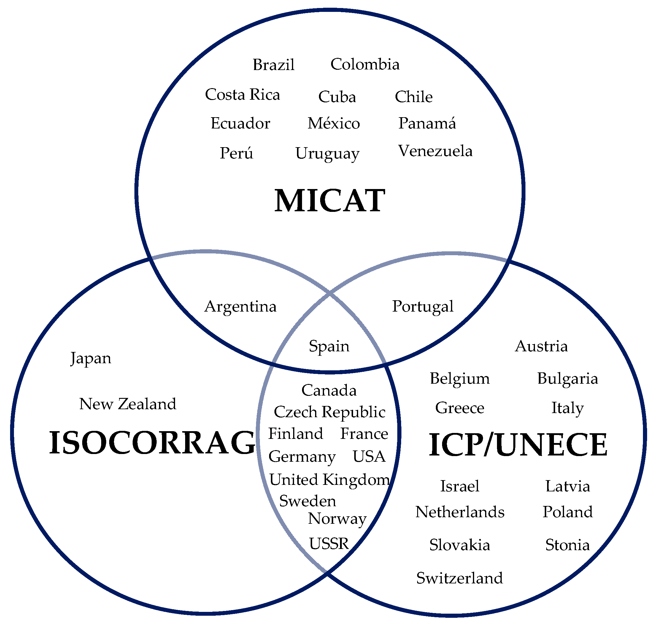
- ISOCORRAG cooperative programme. This programme was designed by the Working Group/WG 4 of ISO 156 Technical Committee “Corrosion of metals and alloys”, with the aim of standardising atmospheric corrosion tests) [1]. The Programme began in the year 1986 and, as a result of the efforts of WG 4, four international standards were developed: ISO 9223 [2,3], ISO 9224 [4], ISO 9225 [5] and ISO 9226 [6]. These standards were based on an extensive review of atmospheric exposure programmes carried out in Europe, North America, and Asia. The aim of drawing up these documents was to establish simple and practical guidelines for the technicians responsible for designing structures to be exposed to the atmosphere and for corrosion engineers responsible for adopting anticorrosive protection measures. ISO 9223 [2] provided a general classification system for atmospheres based either on 1-year coupon exposures or on measurements of environmental parameters to estimate time of wetness (TOW), sulphur dioxide concentration or deposition rate, and sodium chloride deposition rate. ISO 9224 provided an approach to calculating the extent of corrosion damage from extended exposures for five types of engineering metals based on application of guiding corrosion values (average and steady-state corrosion rates) for each corrosivity categories in ISO 9223. ISO 9225 provided the measurements techniques for the sulphur dioxide concentration or deposition rate, and sodium chloride deposition rate, needed as classification criteria in ISO 9223. ISO 9226 provided the procedure for obtaining one-year atmospheric corrosion measurements on standard coupons.
- MICAT cooperative programme: “Ibero-American Atmospheric Corrosivity Map” [7]. The MICAT programme was launched in 1988 as part of the Ibero-American CYTED “Science and Technology for Development” international programme and ended after six years of activities. Fourteen countries participated in the programme, whose goals were: (i) to obtain a greater knowledge of atmospheric corrosion mechanisms in the different environments of Ibero-America; (ii) to establish, by means of suitable statistical analysis of the results obtained, mathematical models that allow the calculation of atmospheric corrosion as a function of climate and pollution parameters; and (iii) to elaborate atmospheric corrosivity maps of the Ibero-American region.
- ICP/UNECE cooperative programme [8]. Airborne acidifying pollutants are known to be one of the major causes of corrosion of different materials, including the extensive damage that has been observed on historic and cultural monuments. In order to fill some important gaps in the knowledge of this field, the Executive Body for the Convention on Long-Range Transboundary Air Pollution (CLRTAP) decided to launch an International Cooperative Programme within the United Nations Economic Commission for Europe (ICP/UNECE). The programme started in September 1987 and initially involved exposure at 39 test sites in 11 European countries and in the United States and Canada. The aim of the programme was to perform a quantitative evaluation of the effect of sulphur pollutants in combination with NOx and other pollutants as well as climatic parameters on the atmospheric corrosion of important materials.
2. Experimental
2.1. ICP/UNECE Programme
2.2. ISOCORRAG Programme
2.3. MICAT Programme
2.4. Analysis of Data Properties
- Extremely cold stations, with annual average temperatures below 0 °C, have been removed from the statistical analysis. Such is the case of the stations at Svanvik (Norway), Murmansk and Ojmjakon (USSR), Jubany (Argentina), Marsch (Chile) and Artigas (Uruguay), the latter three being Antarctic scientific bases. Low temperatures cause the metallic surface to be covered with an ice layer for long time periods during the year, considerably impeding the development of corrosion processes. This ice layer reduces oxygen access to the metallic surface and its time of wetness, decreasing corrosion rates to extremely low values [28,29,30,31].
- In stations characterised as rural environments where SO2 and Cl− deposition rates have not been determined due to being insignificant, values have been estimated for both pollutants. The figures indicated in Table 4, Table 5 and Table 6 correspond to the average value of the 0–3 mg Cl−/m2.d range (level S0) and the 0–4 mg SO2/m2.d range (level P0) according to standard ISO 9223 [3]. In those cases where both pollutants have been estimated, an average of the corrosion data from available annual series has been made.
- For test stations located in non-rural environments, all corresponding annual series data, or even the entirety of the available information, have been removed in those cases where, for some reason, meteorological or pollution data are not included.
- Chloride ion pollution data have not been determined for stations in the ICP/UNECE programme, which only considers non-marine test sites, unlike the other two exposure programmes (ISOCORRAG and MICAT). Therefore, the annual corrosion rate data and meteorological and SO2 deposition rate obtained are only included in the statistical analysis for non-marine environments. In this respect, the criteria adopted has been to remove from the ICP/UNECE database all stations located at a distance of less than 2 km from the seashore, supposing in these cases a chloride ion deposition level of more than 3 mg/m2.d (lower level S1 according to standard ISO 9223 [3]). Bilbao station (Spain), despite being characterised by high SO2 values, has been removed because of its location very close to the port.
2.5. Integration of ICP/UNECE, ISOCORRAG and MICAT Databases
- (a)
- Evaluation of the first-year corrosion (mass loss) of carbon steel according to ISO 9226 [6].
- (b)
- Measurement of meteorological parameters (T, RH, and precipitation) according to standard conventional procedures. The ISOCORRAG programme does not consider precipitation or RH (except at the Czech Republic stations).
- (c)
- (d)
- Measurement of SO2 deposition rate according to ISO 9225 [5].
- (e)
- Measurement of Cl deposition rate according to ISO 9225 [5]. The ICP/UNECE programme does not consider marine atmospheres.
3. Discussion
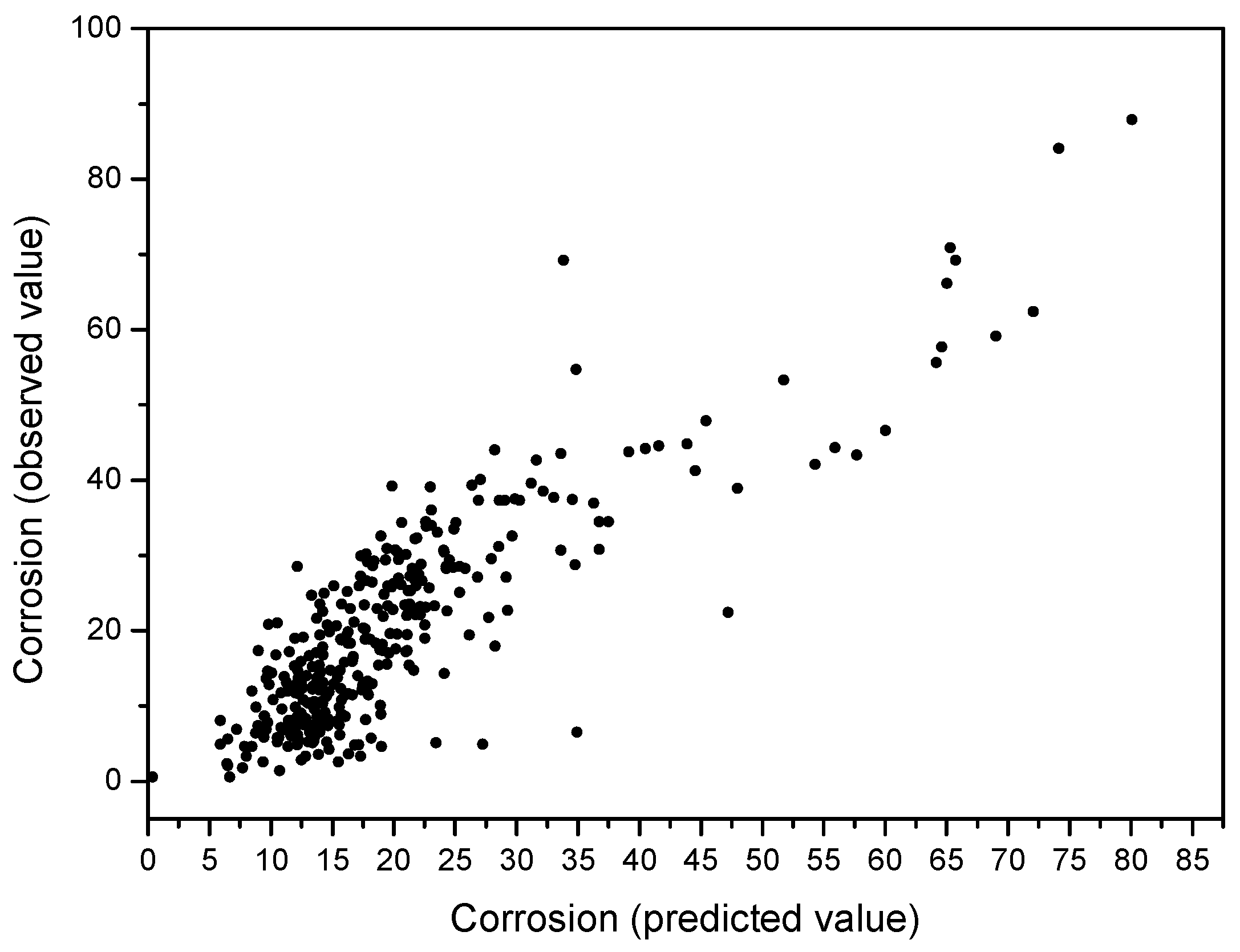
3.1. Non-Marine Atmospheres
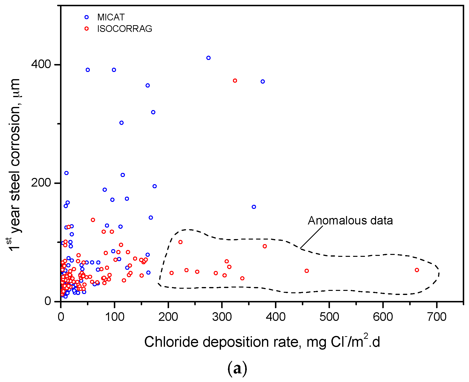
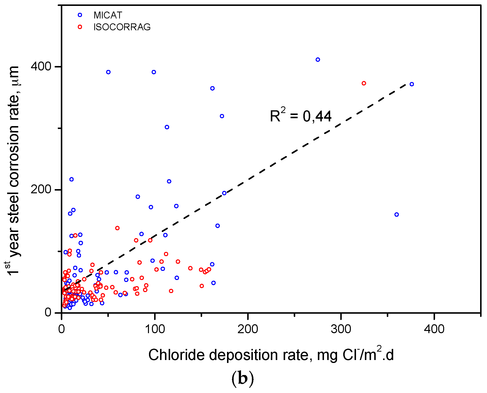
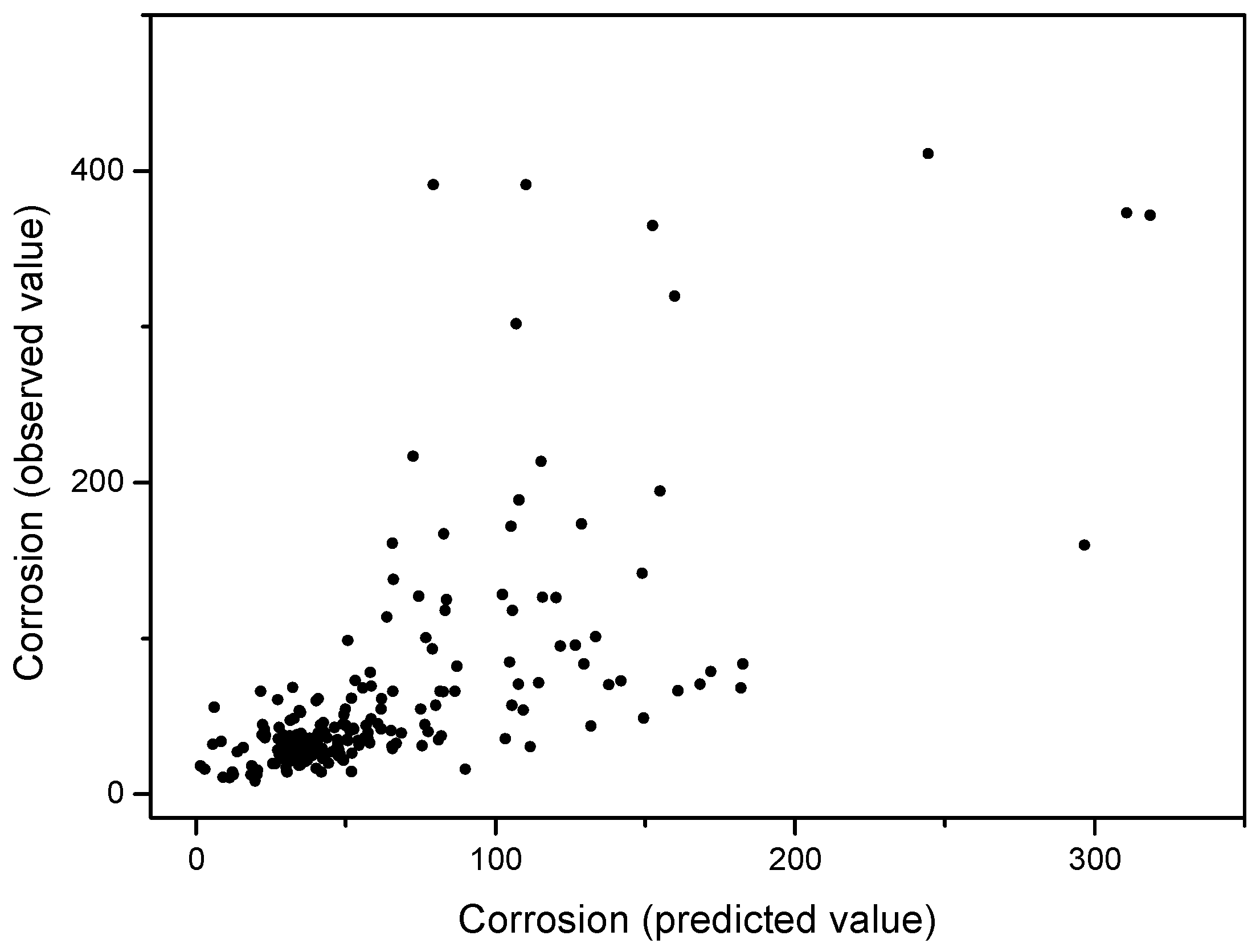
3.2. Marine Atmospheres
3.3. Contribution of the Information Supplied for Each International Programme
4. Goodness of the Fits
- Oversimplification of the mathematical model. In this sense, the best fits obtained in the ISOCORRAG programme, including or excluding the MICAT databases and data from Russian sites in frigid regions [1] (see Table 8), may have been at least partly due to considering interactions between the meteorological and pollution variables. One example of complex interactions involves the RH (or TOW), which in addition to its effect on the wetting of the metal surface, plays a major role in the mechanisms whereby air pollutants take part in corrosion.
- The lack of quality in corrosion and environmental data.
- Probable occurrence of other variables with marked effects on corrosion that were not considered in the statistical treatment. For instance, besides sulphur dioxide and chlorides, other pollutants not considered in the study may have played an important role in the corrosion data. In this sense, mention should be made of the effort made by ICP/UNECE to consider in the new damage functions (for the multi-pollutant situation) other important pollutants in terms of their effect on the corrosion of weathering steel [18].
- Many effects that have not been considered. To mention just a few: The magnitude of diurnal and seasonal changes in meteorological and pollution parameters, the frequency, duration and type of wetting and drying cycles, and the time of year when exposure is initiated.
5. Conclusions
- A highly complete and perfected database has been obtained from published data from the ISOCORRAG, ICP/UNECE and MICAT programmes.
- The number of data used in the statistical treatment has been much higher than that used in other damage functions previously published by the different programmes.
- The statistical treatment carried out has differentiated between two types of atmospheres: non-marine and marine, which may represent a significant simplification for persons with little knowledge of the atmospheric corrosion process who wish to estimate the corrosion of carbon steel exposed at a given location. Moreover, having considered a highly simple polynomial function (Equation (2)) in the work may also be an advantage in this sense.
- With regard to non-marine atmospheres, by joining the three databases (ISOCORRAG, ICP/UNECE and MICAT), the following damage function has been obtained:where SO2 is the variable of greatest significance. The inclusion of TOW (or precipitation) instead of RH leads to lower regression coefficients. The goodness of the fit obtained (R2) is slightly higher than that obtained in the ICP/UNECE programme with a more sophisticated function.C = −26.32 + 0.43 T + 0.45 RH + 0.82 SO2 (R2 = 0.725) (N = 333),
- In relation with marine atmospheres, only the ISOCORRAG and MICAT databases have been considered (ICP/UNECE did not consider this type of atmospheres). The damage function obtained is:where Cl and SO2, in this order, are the most significant variables. The goodness of the fit is slightly lower than that obtained in the MICAT programme, which uses a similar type of function, and notably lower than that obtained in the ISOCORRAG programme using a more sophisticated type of function.C = −24.50 + 0.75 Cl + 0.67 SO2 + 77.32 TOW (R2 = 0.474) (N = 206),
Acknowledgments
Author Contributions
Conflicts of Interest
References
- Knotkova, D.; Kreislova, K.; Dean, S.W.J. ISOCORRAG. International Atmospheric Exposure Program: Summary of Results; ASTM: West Conshohocken, PA, USA, 2010. [Google Scholar]
- Corrosion of Metals and Alloys, Corrosivity of Atmospheres, Classification; ISO 9223: 1992; International Organization for Standardization: Geneva, Switzerland, 1992.
- Corrosion of Metals and Alloys, Corrosivity of Atmospheres, Classification, Determination and Estimation; EN ISO 9223: 2012; European Committee for Standardization: Brussels, Belgium, 2012.
- Corrosion of Metals and Alloys, Corrosivity of Atmospheres, Guiding Values for the Corrosivity Categories; EN ISO 9224: 2012; European Committee for Standardization: Brussels, Belgium, 2012.
- Corrosion of Metals and Alloys, Corrosivity of Atmospheres, Measurement of Environmental Parameters Affecting Corrosivity of Atmospheres; EN ISO 9225: 2012; European Committee for Standardization: Brussels, Belgium, 2012.
- Corrosion of Metals and Alloys, Corrosivity of Atmospheres, Determination of Corrosion Rate of Standard Specimens for the Evaluation of Corrosivity; EN ISO 9226: 2012; European Committee for Standardization: Brussels, Belgium, 2012.
- Morcillo, M.; Almeida, E.; Rosales, B.; Uruchurtu, J.; Marrocos, M. Corrosion y Protección de Metales en las Atmósferas de Iberoamérica. Parte I—Mapas de Iberoamérica de Corrosividad Atmosférica (Proyecto MICAT, XV.1/CYTED); CYTED: Madrid, Spain, 1998. [Google Scholar]
- UN/ECE International Cooperative Programme on Effects on Materials Including Historic and Cultural Monuments, Report n. 01: Technical Manual; Swedish Corrosion Institute: Stockholm, Sweden, 1988.
- Knotkova, D.; Vrobel, L. ISOCORRAG—The International testing program within ISO/TC 156/WG 4. In Proceedings of the 11th International Corrosion Congress; Associazione Italiana di Metallurgia: Florence, Italy, 1990; Volume 5, pp. 581–590. [Google Scholar]
- Kucera, V.; Coote, A.T.; Henriksen, J.F.; Knotkova, D.; Leygraf, C.; Reinhardt, U. Effects of acidifying air pollutants on materials including historic and cultural monuments—An international cooperative programme within unece. In Proceedings of 11th Internacional Corrosion Congress; Associazione Italiana di Metallurgia: Florence, Italy, 1990; Volume 2, pp. 433–442. [Google Scholar]
- Uller, L.; Morcillo, M. The setting-up of an iberoamerican map of atmospheric corrosion. MICAT study-CYTED-D. In Proceedings of the 11th International Corrosion Congress; Associazione Italiana di Metallurgia: Florence, Italy, 1990; pp. 35–45. [Google Scholar]
- United Nations Economic Commission for Europe (UNECE). Effects of Acid Deposition on Atmospheric Corrosion of Materials; Executive Body for the Convention on Long-Range Transboundary Air Pollution, Working Group on Effects: Geneva, Switzerland, 1990. [Google Scholar]
- Benarie, M.; Lipfert, F.L. A general corrosion function in terms of atmospheric pollutant concentrations and rain ph. Atmos. Environ. 1986, 20, 1947–1958. [Google Scholar] [CrossRef]
- Pourbaix, M. The linear bilogaritmic law for atmospheric corrosion. In Atmospheric Corrosion; Ailor, W.H., Ed.; The Electrochemical Society, John Wiley and Sons: New York, NY, USA, 1982; pp. 107–121. [Google Scholar]
- Feliu, S.; Morcillo, M.; Feliu, S., Jr. The prediction of atmospheric corrosion from meteorological and pollution parameters. 1. Annual corrosion. Corros. Sci. 1993, 34, 403–414. [Google Scholar] [CrossRef]
- Feliu, S.; Morcillo, M.; Feliu, S., Jr. The prediction of atmospheric corrosion from meteorological and pollution parameters. 2. Long-term forecasts. Corros. Sci. 1993, 34, 415–422. [Google Scholar] [CrossRef]
- Knotkova, D.; Barton, K. Corrosion aggressivity of atmospheres (derivation and classification). In Atmospheric Corrosion of Metals; Dean, S.W.J., Rhea, E.C., Eds.; American Society for Testing and Materials: Philadelphia, PA, USA, 1982; p. 225. [Google Scholar]
- CLRTAP. Mapping of Effects on Materials, Chapter iv of Manual on Methodologies and Criteria for Modelling and Mapping Critical Loads and Levels and Air Pollution Effects, Risks and Trends. UNECE Convention on Long-Range Transboundary Air Pollution. Available online: www.icpmapping.org (accessed on 1 March 2017).
- McCuen, R.H.; Albrecht, P.; Cheng, J.G. A new approach to power-model regression of corrosion penetration data. In Corrosion Forms and Control for Infrastructure; Chaker, V., Ed.; American Society for Testing and Materials: Philadelphia, PA, USA, 1992; Volume 1137, pp. 46–76. [Google Scholar]
- Albrecht, P.; Hall, T.T. Atmospheric corrosion resistance of structural steels. J. Mater. Civ. Eng. 2003, 15, 2–24. [Google Scholar] [CrossRef]
- Panchenko, Y.M.; Marshakov, A.I. Long-term prediction of metal corrosion losses in atmosphere using a power-linear function. Corros. Sci. 2016, 109, 217–229. [Google Scholar] [CrossRef]
- Panchenko, Y.M.; Marshakov, A.I.; Igonin, T.N.; Kovtanyuk, V.V.; Nikolaeva, L.A. Long-term forecast of corrosion mass losses of technically important metals in various world regions using a power function. Corros. Sci. 2014, 88, 306–316. [Google Scholar] [CrossRef]
- Melchers, R.E. A new interpretation of the corrosion loss processes for weathering steels in marine atmospheres. Corros. Sci. 2008, 50, 3446–3454. [Google Scholar] [CrossRef]
- Melchers, R.E. Long-term corrosion of cast irons and steel in marine and atmospheric environments. Corros. Sci. 2013, 68, 186–194. [Google Scholar] [CrossRef]
- Morcillo, M.; Chico, B.; Díaz, I.; Cano, H.; De la Fuente, D. Atmospheric corrosion data of weathering steels. A review. Corros. Sci. 2013, 77, 6–24. [Google Scholar] [CrossRef]
- Adikari, M.; Munasinghe, N. Development of a corrosion model for prediction of atmospheric corrosion of mild steel. Am. J. Constr. Build. Mater. 2016, 1, 1–6. [Google Scholar]
- Metals and Alloys. Atmospheric Corrosion Testing, General Requirements; ISO 8565; International Organization for Standardization: Geneva, Switzerland, 2011. [Google Scholar]
- Chico, B.; de la Fuente, D.; Morcillo, M. Corrosión atmosférica de metales en condiciones climáticas extremas. Bol. Soc. Esp. Ceram. Vidrio 2000, 39, 329–332. [Google Scholar] [CrossRef]
- Coburn, S.K.; Larrabee, C.P.; Lawson, H.H.; Ellis, O.B. Corrosivennes of various atmospheric test sites as measured by specimens of steel and zinc. In Metal Corrosion in the Atmosphere; American Society for Testing and Materials: Philadelphia, PA, USA, 1968; pp. 360–391. [Google Scholar]
- Biefer, G.J. Atmospheric corrosion of steel in the canadian arctic. Mater. Perform. 1981, 20, 16–19. [Google Scholar]
- Hughes, J.D.; King, G.A.; O’Brien, D.J. Corrosivity in Antarctica—Revelations on the nature of corrosion in the world coldest, driest, highest and purest continent. In Proceedings of the 13th International Corrosion Congress; Australasian Corrosion Association Inc: Melbourne, Australia, 1996. [Google Scholar]
- Alcántara, J.; Chico, B.; Díaz, I.; de la Fuente, D.; Morcillo, M. Airborne chloride deposit and its effect on marine atmospheric corrosion of mild steel. Corros. Sci. 2015, 97, 74–88. [Google Scholar] [CrossRef]
- International Business Machines Corporation. SPSS Statistics, version 23; IBM: North Castle, NY, USA, 2016. [Google Scholar]
- Kreislova, K.; SVUOM, Prague, Czech Republic. Personal communication, 2017.
- Knotkova, D.; Kreislova, K.; Kvapil, J.; Holubova, G.; Bubenickova. CLRTAP, UNECE International Cooperative Programme on Effect on Materials, including Historic and Cultural Monuments, Report No. 42. Results from the Multi-pollutant Programme Corrosion Attack on Carbon Steel after 1, 2 and 4 Years of Exposure (1997–2001); Institute for Protection of Material (SVUOM): Prague, Czech Republic, 2003. [Google Scholar]
- Leygraf, C.; Odnevall Wallinder, I.; Tidblad, J.; Graedel, T. Atmospheric Corrosion, 2nd ed.; The Electrochemical Society Series; John Wiley and Sons: Hoboken, NJ, USA, 2016. [Google Scholar]
- Klassen, R.D.; Roberge, P.R. Aerosol transport modeling as an aid to understanding atmospheric corrosivity patterns. Mater. Des. 1999, 20, 159–168. [Google Scholar] [CrossRef]
- Cole, I.S.; Furman, S.A.; Neufeld, A.K.; Ganther, W.D.; King, G.A. A holistic approach to modelling in atmospheric corrosion. In Proceedings of the 14th International Corrosion Congress; Corrosion Institute of Southern Africa: Cape Town, South Africa, 1999. [Google Scholar]
- Klassen, R.D.; Roberge, P.R. The effects of wind on local atmospheric corrosivity. In Corrosion 2001; NACE International: Houston, TX, USA, 2001. [Google Scholar]
- Roberge, P.R.; Klassen, R.D.; Haberecht, P.W. Atmospheric corrosivity modeling—A review. Mater. Des. 2002, 23, 321–330. [Google Scholar] [CrossRef]


| Code | Country | Test Site | Code | Country | Test Site |
|---|---|---|---|---|---|
| P01 | Czech Republic | Praha | P29 | United Kingdom | Clatteringshaws Loch |
| P02 | Kasperske Hory | P30 | Stoke Orchard | ||
| P03 | Kopisty | P31 | Spain | Madrid | |
| P04 | Finland | Espoo | P32 | Bilbao | |
| P05 | Ahtari | P33 | Toledo | ||
| P06 | Helsinki | P34 | Russia | Moscow | |
| P07 | Germany | Waldhof-Langenbrugge | P35 | Estonia | Lahemaa |
| P08 | Aschaffenburg | P36 | Portugal | Lisbon-Jeronimo Mon. | |
| P09 | Langenfeld-Reusrath | P37 | Canada | Dorset | |
| P10 | Bottrop | P38 | USA | Steubenville | |
| P11 | Essen-Leithe | P39 | Res. Triangle Park | ||
| P12 | Garmisch-Partenkirchen | P40 | France | Paris | |
| P13 | Italy | Rome | P41 | Germany | Berlin |
| P14 | Casaccia | P43 | Israel | Tel Aviv | |
| P15 | Milan | P44 | Norway | Svanvik | |
| P16 | Venice | P45 | Switzerland | Chaumont | |
| P17 | Netherlands | Vlaardingen | P46 | United Kingdom | London |
| P18 | Eibergen | P47 | USA | Los Angeles | |
| P19 | Vredepeel | P49 | Belgium | Anvterps | |
| P20 | Wijnandsrade | P50 | Poland | Katowice | |
| P21 | Norway | Oslo | P51 | Greece | Athens |
| P22 | Borregaard | P52 | Latvia | Riga | |
| P23 | Birkenes | P53 | Austria | Vienna | |
| P24 | Sweden | Stockholm S | P54 | Bulgaria | Sophia |
| P25 | Stockholm C | P55 | Russia | St Petersburg | |
| P26 | Aspvreten | P57 | Finland | Hameelina | |
| P27 | United Kingdom | Lincoln Catch. | P59 | Slovakia | Zilina |
| P28 | Wells. Catch. |
| Code | Country | Test Site | Code | Country | Test Site |
|---|---|---|---|---|---|
| I01 | Argentina | Iguazu | I29 | Norway | Birkenes |
| I02 | Camet | I30 | Tannanger | ||
| I03 | Buenos Aires | I31 | Bergen | ||
| I04 | San Juan | I32 | Svanvik | ||
| I05 | Jubany Base | I33 | Spain | Madrid | |
| I06 | Canada | Bourcherville | I34 | El Pardo | |
| I07 | Czech Republic | Kasperske Hory | I35 | Lagoas-Vigo | |
| I08 | Praha-Bechovice | I36 | Baracaldo, Vizcaya | ||
| I09 | Kopisty | I37 | Sweden | Stockholm-Vanadis | |
| I10 | Germany | Bergisch Gladbach | I38 | Bohus Malmon, Kattesand | |
| I11 | Finland | Helsinki | I39 | Bohus Malmon, Kvarnvik | |
| I12 | Otaniemi | I40 | United Kingdom | Stratford, East London | |
| I13 | Ahtari | I41 | Crowthorne, Berkshire | ||
| I14 | France | Saint Denis | I42 | Rye, East Sussex | |
| I15 | Ponteau Martigues | I43 | Fleet Hall | ||
| I16 | Picherande | I44 | USA | Kure Beach, N. Carolina | |
| I17 | Saint Remy | I45 | Newark-Kerney, New Jersey | ||
| I18 | Salins de Giraud | I46 | Panama Fort Sherman Costal Site | ||
| I19 | Ostende, Belgium | I47 | Research Triangle Park, N. Carolina | ||
| I20 | Paris | I48 | Point Reyes, California | ||
| I21 | Auby | I49 | Los Angeles, California | ||
| I22 | Biarritz | I50 | USSR | Mursmank | |
| I23 | Japan | Choshi | I51 | Batumi | |
| I24 | Tokyo | I52 | Vladivostok | ||
| I25 | Okinawa | I53 | Ojmjakon | ||
| I26 | New Zealand | Judgeford, Wellington | |||
| I27 | Norway | Oslo | |||
| I28 | Borregaard | ||||
| Code | Country | Test Site | Code | Country | Test Site |
|---|---|---|---|---|---|
| M01 | Argentina | Camet | M38 | Ecuador | Esmeraldas |
| M02 | Villa Martelli | M39 | San Cristóbal | ||
| M03 | Iguazú | M40 | Spain | León | |
| M04 | San Juan | M41 | El Pardo | ||
| M05 | Jubany | M42 | Barcelona | ||
| M06 | La Plata | M43 | Tortosa | ||
| M07 | Brazil | Caratinga | M44 | Granada | |
| M08 | Ipatinga | M45 | Lagoas-Vigo | ||
| M09 | Arraial do Cabo | M46 | Labastida | ||
| M10 | Cubatão | M47 | Arties | ||
| M11 | Ubatuba | M48 | México | Mexico | |
| M12 | São Paulo | M49 | Cuernavaca | ||
| M13 | Río de Janeiro | M50 | San Luis Potosí | ||
| M14 | Belem | M51 | Acapulco | ||
| M14 | Fortaleza | M52 | Panamá | Panamá | |
| M16 | Brasilia | M53 | Colon | ||
| M17 | Paulo Afonso | M54 | Veraguas | ||
| M18 | Porto Velho | M55 | Chiriquí | ||
| M19 | Colombia | Isla Naval | M56 | Perú | Piura |
| M20 | San Pedro | M57 | Villa Salvador | ||
| M21 | Cotové | M58 | San Borja | ||
| M22 | Costa Rica | Puntarenas | M59 | Arequipa | |
| M23 | Limón | M60 | Cuzco | ||
| M24 | Arenal | M61 | Pucallpa | ||
| M25 | Sabanilla | M62 | Portugal | Leixões | |
| M26 | Cuba | Ciq | M63 | Sines | |
| M27 | Cojímar | M64 | Pego | ||
| M28 | Bauta | M65 | Uruguay | Trinidad | |
| M29 | Chile | Cerrillos | M66 | Prado | |
| M30 | Valparaíso | M67 | Melo | ||
| M31 | Idiem | M68 | Artigas | ||
| M32 | Petrox | M69 | Punta del Este | ||
| M33 | Marsh | M70 | Venezuela | Tablazo | |
| M34 | Isla de Pascua | M71 | Punto Fijo | ||
| M35 | Ecuador | Guayaquil | M72 | Coro | |
| M36 | Riobamba | M73 | Matanzas | ||
| M37 | Salinas | M74 | Barcelona, V |
| Code | 1st Year Corrosion, µm | T, °C | RH, % | SO2 Deposition Rate mg/m2.d | Precipitation, mm/y | Code | 1st Year Corrosion, µm | T, °C | RH, % | SO2 Deposition Rate, mg/m2.d | Precipitation, mm/y |
|---|---|---|---|---|---|---|---|---|---|---|---|
| P01 | 55.6 | 9.5 | 79 | 62 | 639 | P23 | 12.09 | 6.8 | 77 | 0.16 | 1544 |
| P01 | 34.48 | 9.1 | 73 | 32.96 | 684 | P23 | 5.34 | 6.5 | 82 | 0.16 | 2195 |
| P01 | 30.66 | 9.8 | 77 | 25.68 | 581 | P24 | 33.97 | 7.6 | 78 | 13.44 | 531 |
| P01 | 29.52 | 8.6 | 78 | 18.88 | 475 | P24 | 15.27 | 7 | 70 | 4.56 | 577 |
| P01 | 23.16 | 9.9 | 76 | 12.24 | 522 | P24 | 13.1 | 7.5 | 73 | 3.36 | 581 |
| P01 | 17.56 | 9.5 | 79 | 7.04 | 601 | P24 | 13.61 | 7.4 | 68 | 2.64 | 556 |
| P01 | 13.1 | 9.3 | 72 | 5.12 | 513 | P24 | 15.9 | 6.7 | 76 | 2.08 | 463 |
| P01 | 12.98 | 9.3 | 74 | 8.88 | 491 | P24 | 14.76 | 8.1 | 81 | 1.52 | 635 |
| P01 | 7.51 | 10.1 | 74 | 5.2 | 525 | P24 | 10.31 | 7.1 | 80 | 1.28 | 384 |
| P01 | 8.52 | 10.2 | 70 | 5.12 | 534 | P24 | 11.7 | 8.9 | 74 | 1.44 | 273 |
| P01 | 8.4 | 11 | 73 | 3.68 | 414 | P24 | 7.76 | 7.8 | 76 | 0.64 | 270 |
| P02 | 28.5 | 7 | 77 | 15.76 | 850 | P24 | 5.47 | 7.8 | 77 | 0.72 | 428 |
| P02 | 19.47 | 6.6 | 73 | 14.32 | 921 | P24 | 7.38 | 8.3 | 81 | 0.4 | 330 |
| P02 | 18.83 | 7.2 | 74 | 9.76 | 941 | P25 | 33.46 | 7.6 | 78 | 15.68 | 531 |
| P03 | 70.87 | 9.6 | 73 | 66.64 | 426 | P25 | 13.1 | 7 | 70 | 3.76 | 577 |
| P03 | 44.53 | 8.9 | 71 | 39.2 | 432 | P25 | 12.09 | 7.5 | 73 | 2.72 | 581 |
| P03 | 44.78 | 9.7 | 75 | 39.36 | 513 | P26 | 18.7 | 6 | 83 | 2.64 | 543 |
| P03 | 37.28 | 8.5 | 73 | 24.48 | 431 | P26 | 9.54 | 6 | 81 | 1.04 | 468 |
| P03 | 30.41 | 9.9 | 76 | 14.64 | 420 | P26 | 10.31 | 6.8 | 82 | 0.88 | 525 |
| P03 | 28.5 | 9.2 | 80 | 14.32 | 510 | P26 | 8.78 | 6.5 | 83 | 0.64 | 409 |
| P03 | 23.41 | 8.7 | 73 | 8.96 | 463 | P26 | 7.89 | 5.9 | 86 | 0.48 | 479 |
| P03 | 23.28 | 8.3 | 76 | 14.48 | 442 | P26 | 8.78 | 7.2 | 86 | 0.48 | 772 |
| P03 | 20.74 | 9.3 | 80 | 10.8 | 521 | P26 | 5.09 | 5.6 | 82 | 0.48 | 562 |
| P03 | 28.24 | 9.6 | 79 | 15.2 | 417 | P26 | 5.22 | 6.3 | 84 | 0.48 | 435 |
| P03 | 26.59 | 10.8 | 71 | 9.12 | 433 | P26 | 3.56 | 7.1 | 82 | 0.32 | 452 |
| P04 | 34.48 | 5.9 | 76 | 14.88 | 626 | P26 | 2.54 | 6.7 | 86 | 0.32 | 511 |
| P04 | 16.67 | 5.6 | 79 | 1.84 | 755 | P26 | 14.89 | 7.2 | 82 | 0.24 | 784 |
| P04 | 15.39 | 6 | 80 | 2.08 | 698 | P27 | 40.08 | 9.2 | 84 | 14.16 | 365 |
| P05 | 16.79 | 3.1 | 78 | 5.04 | 801 | P27 | 39.31 | 9.6 | 82 | 14.24 | 530 |
| P05 | 6.11 | 3.4 | 81 | 0.72 | 610 | P27 | 30.15 | 10.5 | 78 | 5.44 | 515 |
| P05 | 7.51 | 3.9 | 83 | 0.64 | 675 | P27 | 34.35 | 10.2 | 81 | 7.5 | 708 |
| P05 | 6.87 | 3.2 | 76 | 0.48 | 618 | P27 | 24.81 | 9.7 | 81 | 6 | 831 |
| P05 | 6.74 | 3.5 | 80 | 0.72 | 742 | P27 | 22.9 | 10.4 | 78 | 3.92 | 548 |
| P05 | 6.49 | 4.8 | 82 | 0.64 | 845 | P28 | 32.19 | 10.8 | 86 | 5.76 | 447 |
| P05 | 4.83 | 4.5 | 80 | 0.64 | 713 | P28 | 25.95 | 10.5 | 82 | 2.56 | 614 |
| P06 | 34.35 | 6.3 | 78 | 16.56 | 673 | P28 | 25.19 | 11.2 | 79 | 2.64 | 696 |
| P06 | 20.74 | 6.2 | 78 | 3.84 | 702 | P30 | 39.06 | 10.2 | 78 | 12 | 610 |
| P06 | 24.94 | 6.6 | 76 | 4.4 | 649 | P30 | 29.26 | 10.3 | 76 | 7.44 | 549 |
| P07 | 33.84 | 9.3 | 80 | 10.96 | 631 | P31 | 28.24 | 14.1 | 66 | 14.72 | 398 |
| P07 | 29.39 | 8.9 | 81 | 6.56 | 624 | P31 | 20.61 | 14.3 | 67 | 6.56 | 360 |
| P07 | 21.12 | 9.5 | 81 | 3.12 | 596 | P31 | 19.21 | 15.7 | 68 | 6.24 | 224 |
| P07 | 19.85 | 8.9 | 82 | 2.32 | 615 | P31 | 20.23 | 14.8 | 67 | 9.12 | 401 |
| P07 | 18.32 | 9.5 | 83 | 1.68 | 786 | P31 | 9.16 | 12.9 | 61 | 9.44 | 765 |
| P07 | 18.83 | 9.4 | 81 | 1.84 | 620 | P31 | 9.8 | 15 | 62 | 0.96 | 560 |
| P07 | 10.81 | 8.8 | 75 | 1.76 | 413 | P31 | 7.38 | 15.3 | 60 | 2.08 | 447 |
| P08 | 27.1 | 12.3 | 77 | 18.96 | 627 | P31 | 5.6 | 15.3 | 56 | 1.28 | 399 |
| P08 | 14.76 | 11.4 | 64 | 10.08 | 561 | P31 | 2.29 | 15.1 | 53 | 2.96 | 267 |
| P08 | 17.81 | 11.6 | 65 | 7.68 | 779 | P31 | 0.51 | 16.2 | 43 | 0.48 | 283 |
| P09 | 37.28 | 10.8 | 77 | 19.6 | 783 | P31 | 2.54 | 16 | 63 | 0.56 | 303 |
| P09 | 29.39 | 10.7 | 79 | 13.04 | 619 | P33 | 5.73 | 14 | 64 | 2.64 | 785 |
| P09 | 26.59 | 11.4 | 81 | 8.88 | 841 | P33 | 3.31 | 13.4 | 61 | 1.36 | 433 |
| P09 | 26.21 | 10 | 78 | 8.4 | 781 | P33 | 4.58 | 14.8 | 57 | 3.36 | 327 |
| P09 | 25.95 | 10.9 | 80 | 6.64 | 930 | P33 | 4.58 | 14 | 61 | 0.88 | 603 |
| P09 | 12.85 | 11.6 | 79 | 4 | 997 | P33 | 6.87 | 14 | 59 | 1.2 | 872 |
| P09 | 16.54 | 11.4 | 76 | 4.8 | 647 | P33 | 5.98 | 12.2 | 71 | 0.96 | 739 |
| P10 | 47.84 | 11.2 | 75 | 40.48 | 874 | P33 | 4.2 | 12.2 | 78 | 0.88 | 411 |
| P10 | 44.15 | 10.3 | 78 | 33.28 | 707 | P33 | 5.73 | 12.1 | 69 | 0.72 | 689 |
| P10 | 37.4 | 11.8 | 80 | 24.16 | 913 | P33 | 1.78 | 14.7 | 61 | 0.32 | 828 |
| P10 | 37.66 | 10.5 | 79 | 23.52 | 806 | P33 | 0.51 | 15.4 | 58 | 0.32 | 430 |
| P10 | 39.57 | 11.5 | 81 | 19.68 | 1044 | P33 | 2.04 | 12.8 | 60 | 0.4 | 516 |
| P10 | 37.28 | 11.7 | 81 | 14.32 | 791 | P34 | 23.03 | 5.5 | 73 | 15.36 | 575 |
| P10 | 28.24 | 11.3 | 77 | 13.52 | 780 | P34 | 17.94 | 5.7 | 74 | 22.96 | 881 |
| P10 | 27.48 | 10.8 | 81 | 8.88 | 663 | P34 | 15.39 | 5.6 | 71 | 13.12 | 667 |
| P10 | 28.63 | 11.1 | 75 | 7.44 | 849 | P34 | 17.18 | 6.5 | 74 | 13.7 | 838 |
| P10 | 30.92 | 11.4 | 78 | 7.04 | 880 | P34 | 17.3 | 7.4 | 69 | 13.7 | 812 |
| P11 | 43.51 | 10.5 | 79 | 24.24 | 713 | P34 | 11.7 | 5.9 | 71 | 3.28 | 750 |
| P11 | 37.28 | 10.1 | 79 | 18.32 | 684 | P35 | 23.54 | 5.5 | 83 | 0.72 | 448 |
| P11 | 30.66 | 10.9 | 78 | 12.96 | 889 | P35 | 13.49 | 5.4 | 82 | 1.1 | 859 |
| P12 | 17.56 | 8 | 82 | 7.52 | 1492 | P35 | 12.09 | 6.9 | 81 | 1.04 | 668 |
| P12 | 11.45 | 7.1 | 84 | 2.56 | 1552 | P35 | 12.21 | 5 | 81 | 1.36 | 655 |
| P12 | 10.81 | 7.4 | 83 | 1.92 | 1503 | P35 | 11.2 | 5.2 | 80 | 3.2 | 403 |
| P13 | 22.65 | 15.4 | 66 | 23.52 | 591 | P35 | 7.38 | 8.8 | 81 | 0.88 | 640 |
| P13 | 15.78 | 18.4 | 68 | 4.64 | 602 | P36 | 28.5 | 12.1 | 64 | 5.44 | 972 |
| P13 | 17.05 | 19.4 | 65 | 2.96 | 1125 | P36 | 39.19 | 18 | 62 | 12.88 | 545 |
| P13 | 8.02 | 17.8 | 53 | 0.88 | 625 | P36 | 25.95 | 19.1 | 67 | 3.76 | 443 |
| P13 | 8.02 | 18 | 66 | 0.64 | 1115 | P36 | 27.23 | 17.9 | 63 | 14.16 | 252 |
| P14 | 29.9 | 14.6 | 71 | 6.64 | 650 | P37 | 18.96 | 5.5 | 75 | 2.64 | 961 |
| P14 | 18.83 | 14.9 | 76 | 4.16 | 717 | P37 | 13.99 | 4.3 | 80 | 1.68 | 1080 |
| P14 | 15.9 | 14.5 | 74 | 4.16 | 742 | P37 | 13.23 | 5.2 | 80 | 2.64 | 1023 |
| P14 | 8.65 | 16.3 | 63 | 0.56 | 600 | P37 | 14.76 | 7.4 | 75 | 1.92 | 788 |
| P14 | 10.81 | 14.5 | 67 | 0.16 | 742 | P37 | 11.96 | 7.2 | 76 | 0.48 | 964 |
| P14 | 6.49 | 15.9 | 69 | 2.96 | 857 | P38 | 27.23 | 14.6 | 69 | 7.68 | 847 |
| P14 | 10.31 | 15.7 | 71 | 0.88 | 585 | P38 | 23.54 | 15.5 | 64 | 8.08 | 982 |
| P14 | 14.38 | 15.5 | 73 | 0.96 | 1114 | P38 | 4.83 | 15.8 | 68 | 7.44 | 1038 |
| P15 | 46.56 | 15.3 | 72 | 57.76 | 1125 | P39 | 22.39 | 12.3 | 67 | 46.48 | 733 |
| P15 | 25.06 | 14.3 | 69 | 17.68 | 1092 | P39 | 36.9 | 11.8 | 65 | 34.48 | 729 |
| P15 | 22.01 | 14.5 | 69 | 12.32 | 1077 | P39 | 6.49 | 11.8 | 69 | 30.64 | 757 |
| P15 | 23.41 | 15.9 | 71 | 10.32 | 932 | P40 | 17.43 | 13.4 | 67 | 11.36 | 572 |
| P15 | 11.45 | 15.1 | 66 | 9.84 | 619 | P40 | 18.19 | 12.7 | 74 | 8.08 | 731 |
| P15 | 14.63 | 14 | 56 | 5.92 | 632 | P40 | 11.96 | 13.3 | 69 | 8.96 | 490 |
| P15 | 11.96 | 15 | 56 | 3.84 | 1179 | P40 | 11.58 | 12.6 | 73 | 5.28 | 571 |
| P15 | 5.85 | 13.9 | 63 | 1.76 | 583 | P40 | 7.51 | 12.7 | 70 | 2.48 | 427 |
| P15 | 8.02 | 15.8 | 63 | 3.52 | 1037 | P40 | 6.11 | 13.2 | 70 | 1.28 | 382 |
| P16 | 31.17 | 14.9 | 77 | 16.88 | 714 | P40 | 8.14 | 13.2 | 74 | 6.2 | 668 |
| P16 | 26.97 | 13.2 | 82 | 5.04 | 500 | P41 | 22.14 | 8.4 | 76 | 13.04 | 473 |
| P16 | 26.84 | 13.5 | 83 | 5.92 | 742 | P41 | 22.77 | 10.4 | 77 | 8.72 | 486 |
| P16 | 18.96 | 14.9 | 83 | 6.24 | 638 | P41 | 22.14 | 11.1 | 82 | 7.84 | 489 |
| P16 | 13.23 | 13.7 | 79 | 3.36 | 795 | P41 | 18.32 | 11.7 | 71 | 6.88 | 473 |
| P16 | 8.78 | 14.5 | 77 | 1.44 | 588 | P41 | 15.52 | 10.1 | 88 | 2.24 | 348 |
| P16 | 9.8 | 15 | 77 | 0.96 | 881 | P41 | 11.58 | 10 | 72 | 2.24 | 570 |
| P17 | 43.77 | 10.5 | 84 | 28.24 | 978 | P41 | 7.38 | 10.3 | 77 | 1.84 | 473 |
| P17 | 38.55 | 10.3 | 83 | 20.4 | 860 | P43 | 41.22 | 24.6 | 83 | 28 | 485 |
| P17 | 32.57 | 11 | 84 | 16.4 | 996 | P43 | 32.57 | 22 | 70 | 5.28 | 254 |
| P18 | 32.32 | 9.9 | 83 | 8.08 | 904 | P45 | 11.83 | 6.2 | 77 | 1.2 | 1135 |
| P18 | 25.95 | 9.5 | 82 | 5.92 | 873 | P45 | 8.52 | 6.9 | 77 | 1.04 | 1053 |
| P18 | 18.32 | 10.3 | 83 | 3.76 | 987 | P45 | 7.38 | 7.2 | 80 | 0.8 | 1281 |
| P19 | 36.01 | 10.3 | 81 | 10.4 | 845 | P45 | 4.58 | 7.3 | 75 | 1.04 | 1011 |
| P19 | 30.41 | 10 | 82 | 6.64 | 749 | P45 | 5.22 | 6.2 | 80 | 0.88 | 1404 |
| P19 | 22.9 | 10.9 | 83 | 3.6 | 829 | P45 | 3.31 | 6.3 | 80 | 0.56 | 950 |
| P20 | 33.08 | 10.3 | 81 | 10.96 | 801 | P45 | 2.8 | 7 | 79 | 0.32 | 1108 |
| P20 | 26.08 | 10.1 | 81 | 7.44 | 680 | P46 | 22.52 | 12.2 | 70 | 4.64 | 706 |
| P20 | 21.88 | 11.1 | 82 | 4.64 | 790 | P46 | 21.63 | 12.1 | 69 | 4.64 | 907 |
| P21 | 29.13 | 7.6 | 70 | 11.52 | 1024 | P46 | 19.08 | 12.7 | 66 | 4.64 | 494 |
| P21 | 17.18 | 7.7 | 68 | 4.8 | 440 | P47 | 17.3 | 17.4 | 61 | 0.48 | 33 |
| P21 | 12.85 | 7.5 | 69 | 2.32 | 680 | P49 | 21.76 | 11.4 | 76 | 18.24 | 834 |
| P21 | 12.6 | 6.8 | 76 | 3.2 | 764 | P49 | 23.54 | 11.7 | 75 | 10.8 | 993 |
| P21 | 11.83 | 6.6 | 79 | 3.28 | 523 | P49 | 13.99 | 11.9 | 65 | 11.04 | 674 |
| P21 | 12.34 | 7.2 | 75 | 2.48 | 1050 | P50 | 34.48 | 9.4 | 81 | 27.52 | 870 |
| P21 | 7.12 | 6.4 | 74 | 1.36 | 794 | P50 | 30.79 | 8.2 | 76 | 30.88 | 702 |
| P21 | 9.54 | 7.2 | 74 | 1.04 | 869 | P50 | 28.75 | 7.5 | 76 | 28.88 | 674 |
| P21 | 7.51 | 6.9 | 76 | 1.6 | 737 | P50 | 28.37 | 7.7 | 84 | 12.24 | 651 |
| P21 | 5.22 | 7.4 | 74 | 0.48 | 715 | P50 | 25.32 | 8.8 | 74 | 12.96 | 676 |
| P21 | 7.89 | 7.5 | 76 | 3.36 | 805 | P50 | 4.58 | 10.7 | 71 | 10.72 | 484 |
| P22 | 54.71 | 6 | 78 | 28.64 | 1116 | P51 | 10.05 | 18.7 | 62 | 11.36 | 461 |
| P22 | 44.02 | 7 | 76 | 21.12 | 628 | P51 | 6.87 | 18.5 | 56 | 3.36 | 325 |
| P22 | 42.62 | 7.4 | 76 | 25.04 | 819 | P51 | 19.85 | 18.7 | 62 | 6.32 | 570 |
| P23 | 24.68 | 6.5 | 80 | 1.04 | 2144 | P52 | 10.56 | 8.2 | 77 | 2.8 | 633 |
| P23 | 16.79 | 5.9 | 75 | 0.56 | 1189 | P52 | 8.02 | 7.8 | 75 | 0.8 | 589 |
| P23 | 13.87 | 6.4 | 76 | 0.56 | 1420 | P53 | 10.43 | 11.2 | 73 | 2 | 855 |
| P23 | 14.38 | 5.6 | 75 | 0.32 | 1182 | P53 | 5.73 | 11.3 | 73 | 2.64 | 555 |
| P23 | 12.85 | 6.2 | 79 | 0.16 | 1744 | P53 | 10.56 | 12 | 71 | 3.36 | 527 |
| P23 | 14.5 | 6.6 | 83 | 0.24 | 2333 | P54 | 8.91 | 11.5 | 70 | 10.8 | 651 |
| P23 | 8.27 | 5.9 | 81 | 0.24 | 1390 | P55 | 12.6 | 6.1 | 76 | 2.48 | 636 |
| P23 | 13.61 | 6.2 | 79 | 0.4 | 1623 | P59 | 13.74 | 9.7 | 74 | 5.2 | 664 |
| P23 | 9.8 | 4.2 | 81 | 0.08 | 1392 |
| Code | 1st Year Corrosion, μm | T, °C | RH, % | TOW, Annual Fraction | Deposition Rates, mg/m2.d | Code | 1st Year Corrosion, μm | T, °C | RH, % | TOW, Annual Fraction | Deposition Rates, mg/m2.d | ||
|---|---|---|---|---|---|---|---|---|---|---|---|---|---|
| SO2 | Cl | SO2 | Cl | ||||||||||
| I01 | 5.8 | 22.9 | 0.615 | 2 | 1.5 | I25 | 54.7 | 24 | 0.478 | 8.48 | 75.85 | ||
| I02 | 24.9 | 14.1 | 0.682 | 2 | 18.21 | I25 | 57.2 | 23.4 | 0.439 | 8.84 | 86.17 | ||
| I02 | 54.8 | 13.9 | 0.708 | 2 | 24.39 | I25 | 44.8 | 23.2 | 0.338 | 9.76 | 91.03 | ||
| I02 | 78.2 | 14.3 | 0.725 | 2 | 33.38 | I25 | 39.2 | 23.5 | 0.354 | 10.4 | 78.89 | ||
| I02 | 66 | 14.5 | 0.736 | 2 | 42.48 | I27 | 26.1 | 6.7 | 0.299 | 13.84 | 1.21 | ||
| I02 | 68.3 | 14.2 | 0.711 | 2 | 32.16 | I27 | 26.6 | 6.2 | 0.326 | 11.84 | 2.18 | ||
| I03 | 14.7 | 17.1 | 0.529 | 9.7 | 1.5 | I27 | 30.2 | 7.4 | 0.279 | 11.28 | 1.58 | ||
| I04 | 4.6 | 19.2 | 0.104 | 2 | 1.5 | I27 | 21.5 | 8.5 | 0.261 | 12.64 | 0.73 | ||
| I06 | 25.5 | 8 | 0.287 | 11.28 | 33.38 | I27 | 26.5 | 7.9 | 0.297 | 9.92 | 0.91 | ||
| I06 | 21.5 | 7.6 | 0.267 | 12.8 | 42.48 | I27 | 20.1 | 8.5 | 0.346 | 6.8 | 1.03 | ||
| I06 | 28.3 | 8 | 0.238 | 12.4 | 33.38 | I28 | 68.4 | 4.9 | 0.358 | 34.4 | 8.01 | ||
| I06 | 21.3 | 7.5 | 0.283 | 12.24 | 37.02 | I28 | 60.8 | 5.4 | 0.365 | 28.8 | 5.22 | ||
| I06 | 25.5 | 7 | 0.287 | 12.72 | 35.2 | I28 | 66 | 5.7 | 0.313 | 28.8 | 4.01 | ||
| I06 | 21.6 | 7 | 0.317 | 14.8 | 33.98 | I28 | 60 | 7.5 | 0.407 | 41.6 | 6.86 | ||
| I07 | 27.1 | 5.5 | 76 | 0.347 | 20.24 | 2.31 | I28 | 61.4 | 6.6 | 0.423 | 42.4 | 6.07 | |
| I07 | 23.1 | 7.1 | 77 | 0.414 | 13.68 | 1.64 | I28 | 53.6 | 6.7 | 0.42 | 36.16 | 3.22 | |
| I07 | 26 | 6.8 | 77 | 0.409 | 12.88 | 2 | I29 | 21.4 | 5.2 | 0.42 | 1.44 | 0.61 | |
| I07 | 23.3 | 7.1 | 76 | 0.353 | 10.48 | 2 | I29 | 18.6 | 5.9 | 0.526 | 0.96 | 0.61 | |
| I07 | 30.7 | 7 | 77 | 0.454 | 10.72 | 2 | I29 | 21.8 | 6.3 | 0.478 | 0.96 | 0.61 | |
| I07 | 25.7 | 7.3 | 77 | 0.503 | 13.92 | 2 | I29 | 17.1 | 7.5 | 0.503 | 0.8 | 0.61 | |
| I08 | 62.4 | 7.5 | 81 | 0.272 | 71.6 | 2.91 | I29 | 20.7 | 6.6 | 0.453 | 0.8 | 0.61 | |
| I08 | 44.3 | 8.8 | 79 | 0.285 | 52.32 | 1.21 | I29 | 18.6 | 6.2 | 0.42 | 0.8 | 0.61 | |
| I08 | 43.3 | 9.3 | 75 | 0.238 | 56.4 | 2.1 | I31 | 27.2 | 7.2 | 0.372 | 7.84 | 2.61 | |
| I08 | 42.1 | 9.7 | 74 | 0.226 | 52.64 | 2.1 | I31 | 22.3 | 7.7 | 0.443 | 7.92 | 2.06 | |
| I08 | 53.3 | 9.9 | 77 | 0.264 | 47.76 | 2.1 | I31 | 27.7 | 8.2 | 0.495 | 7.92 | 2.12 | |
| I08 | 38.9 | 10.1 | 77 | 0.299 | 43.04 | 2.1 | I31 | 25.7 | 8.9 | 0.557 | 5.68 | 6.98 | |
| I09 | 87.9 | 7.7 | 76 | 0.355 | 84 | 2.31 | I31 | 38 | 8.4 | 0.584 | 5.44 | 6.92 | |
| I09 | 66.1 | 9 | 73 | 0.279 | 66.64 | 1.09 | I31 | 26.3 | 8.4 | 0.59 | 6.4 | 4.85 | |
| I09 | 57.7 | 9.5 | 73 | 0.256 | 65.84 | 1.7 | I33 | 31.9 | 14.1 | 0.15 | 22 | 1.5 | |
| I09 | 59.1 | 9.8 | 72 | 0.266 | 71.6 | 1.7 | I33 | 29.8 | 14.3 | 0.201 | 24.24 | 1.5 | |
| I09 | 84.1 | 9.6 | 74 | 0.271 | 76.88 | 1.7 | I33 | 33.2 | 12.5 | 0.301 | 36.88 | 1.5 | |
| I09 | 69.2 | 9.9 | 74 | 0.235 | 66.48 | 1.7 | I33 | 22.4 | 14.1 | 0.277 | 41.2 | 1.5 | |
| I10 | 38.5 | 10.4 | 0.545 | 18.72 | 1.52 | I33 | 26.1 | 14.9 | 0.227 | 43.2 | 1.5 | ||
| I10 | 40.6 | 10.8 | 0.535 | 17.84 | 1.09 | I33 | 22.7 | 14.9 | 0.254 | 44.48 | 1.5 | ||
| I10 | 35.3 | 11.1 | 0.506 | 12.08 | 1.09 | I34 | 16.3 | 25.3 | 0.277 | 3.12 | 1.5 | ||
| I10 | 37.4 | 10.8 | 0.486 | 10.56 | 1.4 | I34 | 17 | 25.3 | 0.31 | 3.84 | 1.5 | ||
| I10 | 31.8 | 9.6 | 0.428 | 14.64 | 1.03 | I34 | 17.4 | 25.3 | 0.418 | 4.64 | 1.5 | ||
| I10 | 33.8 | 9.7 | 0.424 | 12.48 | 0.61 | I34 | 12.9 | 25.3 | 0.359 | 4.32 | 1.5 | ||
| I11 | 37.5 | 3.3 | 0.339 | 17.12 | 2.18 | I34 | 15.6 | 25.2 | 0.402 | 3.28 | 1.5 | ||
| I11 | 33 | 5.1 | 0.395 | 17.12 | 2.49 | I34 | 13.7 | 25.5 | 0.442 | 4.32 | 1.5 | ||
| I11 | 41.2 | 6.4 | 0.394 | 16 | 2.55 | I35 | 34.4 | 15.2 | 0.365 | 49.28 | 18.21 | ||
| I11 | 28.3 | 6.8 | 0.42 | 14.72 | 2.43 | I35 | 24.7 | 16.2 | 0.374 | 38.88 | 11.53 | ||
| I11 | 31.4 | 6.7 | 0.439 | 13.28 | 2.41 | I35 | 25.2 | 16.2 | 0.31 | 37.2 | 12.14 | ||
| I11 | 28.6 | 6.8 | 0.464 | 12.24 | 2.41 | I35 | 27.6 | 15.8 | 0.293 | 35.84 | 11.53 | ||
| I12 | 30.9 | 3 | 0.297 | 16.24 | 2.55 | I35 | 22.7 | 16.6 | 0.31 | 37.04 | 12.14 | ||
| I12 | 21.4 | 4.9 | 0.325 | 13.04 | 1.52 | I35 | 26.8 | 17.2 | 0.293 | 35.68 | 11.53 | ||
| I12 | 34.6 | 5.4 | 0.388 | 15.2 | 1.09 | I36 | 45.9 | 14.5 | 0.492 | 29.44 | 12.74 | ||
| I12 | 19.9 | 5.3 | 0.348 | 11.2 | 1.72 | I36 | 51.1 | 15.8 | 0.493 | 34.24 | 17.6 | ||
| I12 | 26.2 | 5.9 | 0.434 | 8.48 | 1.72 | I36 | 45 | 16.7 | 0.517 | 31.04 | 16.99 | ||
| I12 | 20.8 | 6.4 | 0.491 | 9.04 | 1.72 | I36 | 44.3 | 16.2 | 0.511 | 23.52 | 14.56 | ||
| I13 | 16.7 | 0.3 | 0.378 | 4.72 | 1.94 | I36 | 33.3 | 16.1 | 0.464 | 16.8 | 24.27 | ||
| I13 | 11 | 2.2 | 0.345 | 4.24 | 1.5 | I37 | 28 | 5 | 0.29 | 8.16 | 1.5 | ||
| I13 | 15.7 | 3.4 | 0.313 | 4.08 | 1.5 | I37 | 26.9 | 6.8 | 0.416 | 8.8 | 1.5 | ||
| I13 | 9.7 | 4 | 0.347 | 2.8 | 1.5 | I37 | 28.1 | 7.1 | 0.359 | 9.6 | 1.5 | ||
| I13 | 12.5 | 4 | 0.357 | 2.48 | 1.5 | I37 | 21.6 | 8 | 0.347 | 8 | 1.5 | ||
| I13 | 11.3 | 4.1 | 0.386 | 1.52 | 1.5 | I37 | 23.5 | 8.4 | 0.338 | 8.8 | 1.5 | ||
| I14 | 40.7 | 12.3 | 0.473 | 42.24 | 15.17 | I37 | 18.1 | 8.4 | 0.385 | 5.6 | 1.5 | ||
| I14 | 34.5 | 13.1 | 0.546 | 37.04 | 15.17 | I38 | 43 | 6.1 | 0.447 | 7.04 | 41.87 | ||
| I14 | 44.2 | 13.5 | 0.52 | 31.04 | 18.21 | I38 | 28.8 | 8 | 0.472 | 4 | 44.3 | ||
| I14 | 35 | 13 | 0.511 | 32 | 18.81 | I38 | 33.1 | 8.7 | 0.462 | 6.4 | 30.95 | ||
| I15 | 83.5 | 14.6 | 0.423 | 120.8 | 125.01 | I38 | 33.3 | 9.5 | 0.454 | 1.6 | 58.26 | ||
| I15 | 68.1 | 16.2 | 0.488 | 77.04 | 155.96 | I38 | 41.8 | 9.5 | 0.449 | 2.4 | 54.62 | ||
| I15 | 70.7 | 16.1 | 0.427 | 61.04 | 158.38 | I38 | 31.2 | 9.7 | 0.474 | 4 | 81.32 | ||
| I15 | 66.4 | 15.6 | 0.349 | 64 | 154.14 | I40 | 42.3 | 11.4 | 0.705 | 20.56 | 11.41 | ||
| I15 | 72.6 | 15.6 | 0.503 | 35.84 | 138.36 | I40 | 35.1 | 11.4 | 0.66 | 16.56 | 12.86 | ||
| I16 | 19.6 | 6.5 | 0.493 | 14.4 | 4.85 | I40 | 36 | 11.4 | 0.631 | 14.32 | 5.58 | ||
| I16 | 15.5 | 6.5 | 0.474 | 9.04 | 3.64 | I40 | 37.6 | 11.4 | 0.547 | 13.84 | 5.16 | ||
| I16 | 19.6 | 7.1 | 0.542 | 8 | 4.25 | I40 | 42.9 | 11.4 | 0.467 | 15.2 | 7.83 | ||
| I16 | 12.3 | 6.7 | 0.47 | 6.48 | 3.03 | I40 | 38 | 11.4 | 0.512 | 14.8 | 12.02 | ||
| I18 | 82.1 | 13.6 | 0.352 | 32.5 | 83.74 | I41 | 36.4 | 10.5 | 0.687 | 12.88 | 8.56 | ||
| I18 | 70.2 | 14.2 | 0.37 | 32 | 149.89 | I43 | 39.6 | 9 | 0.707 | 15.36 | 3.22 | ||
| I18 | 70.5 | 15.4 | 0.45 | 31.44 | 101.95 | I43 | 35.4 | 9 | 0.68 | 13.6 | 2.31 | ||
| I19 | 118 | 9.7 | 0.691 | 8 | 95.27 | I43 | 38.1 | 9 | 0.449 | 12.88 | 4.43 | ||
| I19 | 95.8 | 9.7 | 0.664 | 24 | 112.26 | I43 | 41.7 | 9 | 0.459 | 12.88 | 4.43 | ||
| I19 | 83.5 | 9.7 | 0.728 | 25.6 | 107.41 | I43 | 41.8 | 9 | 0.545 | 13.12 | 2.06 | ||
| I20 | 37.6 | 13 | 0.494 | 42.88 | 1.5 | I43 | 37.7 | 9 | 0.491 | 11.36 | 3.09 | ||
| I20 | 39.7 | 13 | 0.38 | 42.88 | 1.5 | I44 | 40.2 | 13.3 | 0.503 | 4.32 | 80.71 | ||
| I20 | 48 | 13 | 0.218 | 42.4 | 1.5 | I44 | 32.5 | 18.1 | 0.479 | 4.96 | 67.97 | ||
| I21 | 101 | 9.6 | 0.471 | 171.68 | 8.92 | I44 | 37.6 | 17.8 | 0.464 | 5.28 | 89.81 | ||
| I21 | 95.1 | 11.9 | 0.527 | 147.68 | 8.5 | I44 | 35.6 | 17.4 | 0.473 | 4.88 | 117.73 | ||
| I21 | 126 | 12.8 | 0.567 | 133.6 | 14.93 | I44 | 43.8 | 18.2 | 0.492 | 8.4 | 150.5 | ||
| I23 | 44 | 16 | 0.654 | 5.84 | 36.41 | I45 | 26.4 | 11.8 | 0.216 | 26.3 | 1.5 | ||
| I23 | 40.9 | 15.9 | 0.639 | 6.48 | 47.94 | I46 | 373 | 27.3 | 0.824 | 42.4 | 324.66 | ||
| I23 | 45.2 | 15.5 | 0.644 | 6.64 | 41.87 | I51 | 32.2 | 13.2 | 0.364 | 20 | 0.61 | ||
| I23 | 39.7 | 15.8 | 0.643 | 6.48 | 37.62 | I51 | 33.6 | 13.4 | 0.341 | 22.56 | 0.61 | ||
| I23 | 48.2 | 16.1 | 0.644 | 6 | 39.44 | I51 | 29.4 | 13.1 | 0.395 | 20.48 | 0.61 | ||
| I23 | 42.1 | 16.2 | 0.683 | 5.68 | 40.05 | I51 | 30.2 | 13.3 | 0.386 | 21.2 | 0.61 | ||
| I24 | 38 | 14.1 | 0.18 | 11.28 | 2.61 | I51 | 22.5 | 13.7 | 0.383 | 21.12 | 0.67 | ||
| I24 | 28.6 | 14.1 | 0.221 | 11.6 | 2.49 | I51 | 24.2 | 13.3 | 0.334 | 20.8 | 0.61 | ||
| I24 | 48.8 | 13.9 | 0.275 | 11.28 | 2.85 | I52 | 39 | 3.9 | 0.465 | 10.4 | 21.85 | ||
| I24 | 32.1 | 14 | 0.262 | 11.36 | 3.34 | I52 | 26.4 | 4.2 | 0.434 | 12.64 | 14.56 | ||
| I24 | 55.8 | 14.2 | 0.258 | 12.24 | 3.16 | I52 | 22.4 | 5.8 | 0.405 | 27.44 | 11.23 | ||
| I24 | 33.8 | 14.6 | 0.291 | 12.4 | 3.09 | I52 | 23.9 | 5.9 | 0.396 | 32.88 | 6.68 | ||
| I25 | 118 | 22.8 | 0.538 | 8.88 | 80.1 | I52 | 17.4 | 6.8 | 0.483 | 20.32 | 5.28 | ||
| I25 | 138 | 23.9 | 0.525 | 6.64 | 60.08 | I52 | 26.3 | 6.2 | 0.503 | 22.32 | 7.34 | ||
| Code | 1st Year Corrosion, μm | T, °C | RH, % | TOW, Annual Fraction | Precipitation, mm/y | Deposition Rates, mg/m2.d | |
|---|---|---|---|---|---|---|---|
| SO2 | Cl | ||||||
| M01 | 54.8 | 13.9 | 79 | 0.708 | 805 | 2 | 40.2 |
| M01 | 66 | 14.5 | 80 | 0.736 | 1226 | 2 | 70 |
| M02 | 14.73 | 16.9 | 74 | 0.538 | 1377 | 9 | 1.5 |
| M03 | 5.7 | 21.2 | 75 | 0.643 | 2167 | 2 | 1.50 |
| M04 | 4.9 | 18.8 | 50 | 0.103 | 80 | 2 | 1.50 |
| M06 | 25.3 | 17 | 78 | 0.593 | 1178 | 6.2 | 1.5 |
| M06 | 28.8 | 16.7 | 77 | 0.565 | 1263 | 8.2 | 1.5 |
| M06 | 30.1 | 16.6 | 78 | 0.631 | 1361 | 6.2 | 1.5 |
| M07 | 8.6 | 21.5 | 74 | 0.482 | 847 | 0.8 | 8.9 |
| M07 | 11.5 | 20.9 | 75 | 0.482 | 1167 | 1.3 | 7.4 |
| M07 | 13.1 | 21.2 | 75 | 0.482 | 996 | 1.7 | 1.60 |
| M08 | 52.5 | 23.8 | 89 | 0.482 | 1122 | 23.8 | 8.6 |
| M08 | 47.3 | 22.9 | 91 | 0.482 | 1471 | 20.7 | 6.8 |
| M08 | 48.5 | 23 | 90 | 0.482 | 1444 | 24.5 | 5.2 |
| M09 | 159.8 | 24.8 | 77 | 0.582 | 605 | 9.5 | 359.8 |
| M09 | 194.7 | 24.5 | 79 | 0.582 | 985 | 5.3 | 174.8 |
| M09 | 141.7 | 24.2 | 77 | 0.582 | 716 | 4.4 | 167.70 |
| M10 | 98.7 | 22.7 | 73 | 0.579 | 960 | 40.4 | 4.50 |
| M10 | 161.2 | 22.9 | 71 | 0.579 | 870 | 57.4 | 9.20 |
| M10 | 216.9 | 22.6 | 79 | 0.579 | 1133 | 65.8 | 10.80 |
| M11 | 301.9 | 22.1 | 80 | 0.579 | 1689 | 2.6 | 113.20 |
| M13 | 127.1 | 20.1 | 80 | 0.598 | 1353 | 55.85 | 20.21 |
| M13 | 61.2 | 23.1 | 78 | 0.598 | 1369 | 44.09 | 14.22 |
| M13 | 73.1 | 21 | 82 | 0.598 | 1305 | 30.51 | 14.67 |
| M14 | 19.4 | 26.1 | 88 | 0.682 | 2395 | 2 | 1.50 |
| M16 | 12.9 | 20.4 | 69 | 0.442 | 1440 | 2 | 1.50 |
| M17 | 17.3 | 25.9 | 77 | 0.172 | 1392 | 2 | 1.50 |
| M18 | 4.9 | 26.6 | 90 | - | 2096 | 2 | 1.50 |
| M19 | 16 | 27.6 | 85 | 0.989 | 940 | 7.8 | 43.60 |
| M19 | 30.6 | 27.6 | 87 | 0.966 | 940 | 14.2 | 69.00 |
| M19 | 54 | 28.2 | 87 | 0.975 | 940 | 8.9 | 69.50 |
| M20 | 17 | 11.5 | 90 | 1 | 1800 | 0.6 | 1.50 |
| M21 | 19.6 | 27 | 76 | 0.33 | 900 | 0.3 | 1.50 |
| M22 | 61.6 | 27.6 | 80 | 0.562 | 1598 | 6.3 | 38.7 |
| M23 | 371.5 | 25.3 | 88 | 0.763 | 3531 | 3.5 | 376 |
| M24 | 69.3 | 22.9 | 88 | 0.838 | 3677 | 4 | 20.60 |
| M25 | 16.6 | 18.9 | 83 | 0.695 | 1780 | 2.4 | 12.10 |
| M26 | 36.1 | 25.2 | 80 | 0.571 | 1591 | 37.1 | 15.8 |
| M26 | 26.4 | 25.4 | 79 | 0.571 | 1303 | 36.5 | 10.9 |
| M26 | 29 | 24.7 | 79 | 0.571 | 1321 | 19.8 | 10.9 |
| M26 | 32.3 | 25.5 | 79 | 0.571 | 1129 | 25.6 | 14.3 |
| M26 | 31.3 | 25.4 | 79 | 0.571 | 1305 | 41 | 10.10 |
| M26 | 29.2 | 24.7 | 79 | 0.571 | 1540 | 24.7 | 8.20 |
| M26 | 27.3 | 25.2 | 79 | 0.571 | 1415 | 18.5 | 18.10 |
| M26 | 32.8 | 25.1 | 79 | 0.571 | 1064 | 49.2 | 7.40 |
| M27 | 391.1 | 25.2 | 80 | 0.571 | 1591 | 24.5 | 99.10 |
| M27 | 213.7 | 25.4 | 79 | 0.571 | 1303 | 13.5 | 115.60 |
| M27 | 173.6 | 24.7 | 79 | 0.571 | 1321 | 25.1 | 123.30 |
| M27 | 171.9 | 25.5 | 79 | 0.571 | 1129 | 20.4 | 96.00 |
| M27 | 391.2 | 25 | 79 | 0.571 | 1108 | 32.8 | 50.40 |
| M27 | 126.5 | 25.4 | 79 | 0.571 | 1305 | 18.9 | 111.40 |
| M27 | 71.6 | 25.7 | 79 | 0.571 | 1540 | 19.9 | 108.80 |
| M27 | 84.8 | 24.2 | 79 | 0.571 | 1415 | 17.7 | 97.70 |
| M27 | 188.9 | 25.1 | 80 | 0.571 | 1064 | 40.4 | 81.80 |
| Type of Atmosphere | Variable | Smallest Value | Largest Value |
|---|---|---|---|
| Non marine | C (µm) | 0.51 | 87.9 |
| T (°C) | 3.1 | 27 | |
| RH (%) | 35 | 90 | |
| SO2 (mg/m2.d) | 0.08 | 84 | |
| Marine | C (µm) | 8.6 | 411.2 |
| T (°C) | 3.9 | 28.2 | |
| TOW (annual fraction) | 0.16 | 0.99 | |
| SO2 (mg/m2.d) | 0.3 | 171.7 | |
| Cl (mg/m2.d) | 3.03 | 376 |
| Type of Atmosphere | Programme | Ref. | D/R Function | N | R2 |
|---|---|---|---|---|---|
| Non marine | ICP/UNECE (for weathering steels) | [18] | C = 34[SO2]0.13 exp{0.020 RH + f(T)} where f(T) = 0.059(T − 10) when T ≤ 10 °C, otherwise f(T) = −0.036 (T − 10) | 148 | 0.68 |
| All atmospheres (marine and non-marine atmospheres) | ISOCORRAG | [35] | C = 0.091 [SO2]0.56 TOW0.52 exp(f(T)) + 0.158[Cl]0.58 TOW0.25 exp(0.050 T) where f(T) = 0.103 (T − 10) when T ≤ 10 °C, otherwise f(T) = −0.059 (T − 10) | 125 | 0.85 |
| C = 1.77 [SO2]0.52 exp(0.020 RH) exp(f(T)) +0.102[Cl]0.62 exp(0.033 RH +0.040 T) where f(T) = 0.150 (T − 10) when T ≤ 10 °C, otherwise f(T) = −0.054 (T − 10) | 128 | 0.85 | |||
| MICAT | [7] | C = −0.44 + 6.38 TOW + 1.58[SO2] + 0.96[Cl] | 172 | 0.56 | |
| ISOCORRAG/MICAT Including data from Russian sites in frigid regions | [1] | C = 0.085 × SO20.56 × TOW0.53 × exp(f) + 0.24 × Cl0.47 × TOW0.25 × exp(0.049 T) f(T) = 0.098 (T − 10) when T ≤ 10 °C, otherwise f(T) = −0.087 (T − 10) | 119 | 0.87 |
| Type of Atmosphere | Programme | N | Significant Variables | D/R Function | R2 |
|---|---|---|---|---|---|
| Non-marine atmospheres | Overall D/R function (Equation (3)) (ICP/UNECE + ISOCORRAG + MICAT) | 333 | SO2, RH, T | C= 0.82 SO2 + 0.26 RH + 0.15 T | 0.725 |
| ICP/UNECE | 269 | SO2, RH, T | C= 0.74 SO2 + 0.37 RH + 0.21 T | 0.674 | |
| ISOCORRAG | 18 | SO2 | C= 0.93 SO2 | 0.867 | |
| MICAT | 46 | SO2, T | C= 0.49 SO2 + 0.46 T | 0.398 | |
| Marine atmospheres | Overall D/R function (Equation (7)) (ISOCORRAG + MICAT) | 206 | Cl, SO2, TOW | C= 0.62 Cl + 0.22 SO2 + 0.15 TOW | 0.474 |
| ISOCORRAG | 97 | Cl, SO2, TOW | C= 0.57 Cl + 0.31 SO2 + 0.31 TOW | 0.582 | |
| MICAT | 109 | Cl, SO2, | C= 0.69 Cl + 0.30 SO2 | 0.538 |
© 2017 by the authors. Licensee MDPI, Basel, Switzerland. This article is an open access article distributed under the terms and conditions of the Creative Commons Attribution (CC BY) license (http://creativecommons.org/licenses/by/4.0/).
Share and Cite
Chico, B.; De la Fuente, D.; Díaz, I.; Simancas, J.; Morcillo, M. Annual Atmospheric Corrosion of Carbon Steel Worldwide. An Integration of ISOCORRAG, ICP/UNECE and MICAT Databases. Materials 2017, 10, 601. https://doi.org/10.3390/ma10060601
Chico B, De la Fuente D, Díaz I, Simancas J, Morcillo M. Annual Atmospheric Corrosion of Carbon Steel Worldwide. An Integration of ISOCORRAG, ICP/UNECE and MICAT Databases. Materials. 2017; 10(6):601. https://doi.org/10.3390/ma10060601
Chicago/Turabian StyleChico, Belén, Daniel De la Fuente, Iván Díaz, Joaquín Simancas, and Manuel Morcillo. 2017. "Annual Atmospheric Corrosion of Carbon Steel Worldwide. An Integration of ISOCORRAG, ICP/UNECE and MICAT Databases" Materials 10, no. 6: 601. https://doi.org/10.3390/ma10060601