A Time-Variant Reliability Model for Copper Bending Pipe under Seawater-Active Corrosion Based on the Stochastic Degradation Process


Abstract
:
1. Introduction
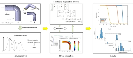
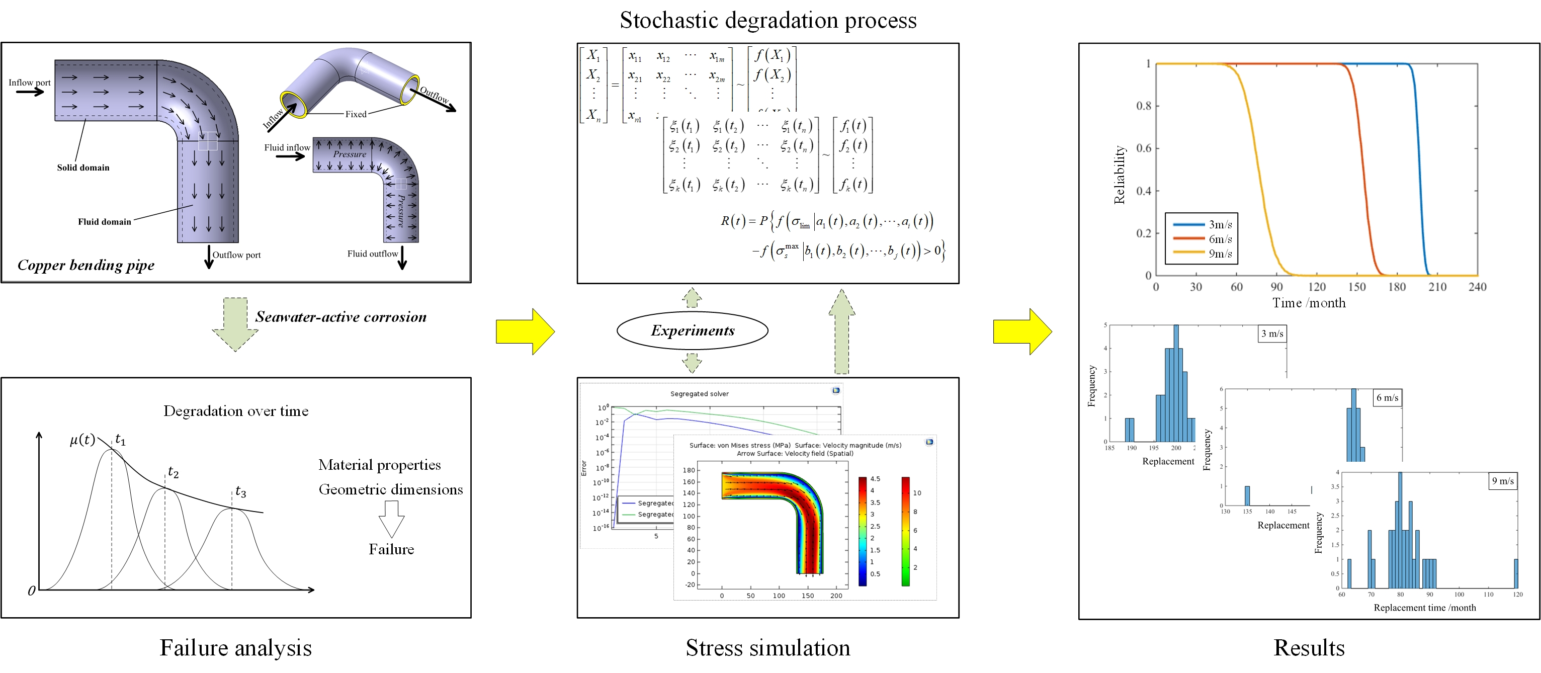
2. Time-Variant Reliability Modeling Method
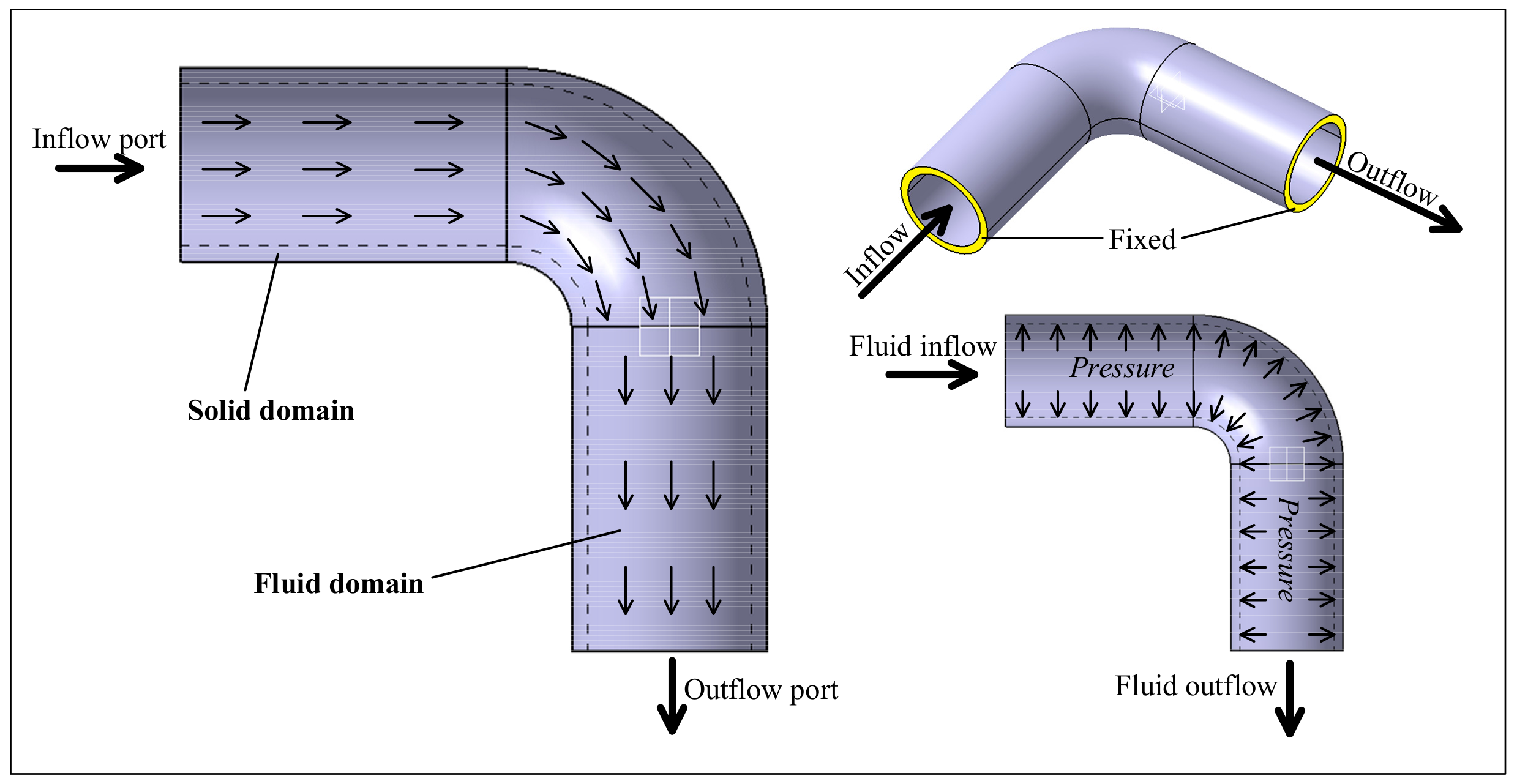
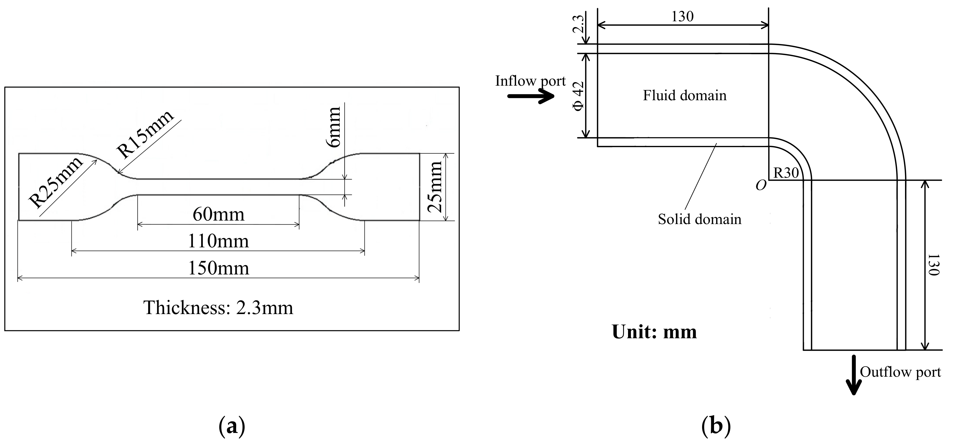
2.1. Failure Analysis of Copper Bending Pipe
2.2. Stochastic Degradation Process Based on Modeling Method
- (1)
- The thickness of the copper bending pipe is equal, regardless of the residual stresses during the forming process.
- (2)
- Copper materials are assumed to be a material with uniform elastic properties; the Young’s modulus and Poisson’s ratio are not degraded.
- (3)
- The fixed constraint of copper bending pipe is completely reliable. This means that the copper bending pipe will not fall off in any case.
2.3. Solution for Reliability Model
3. Experiments and Reliability Analysis
3.1. Experiment Setup
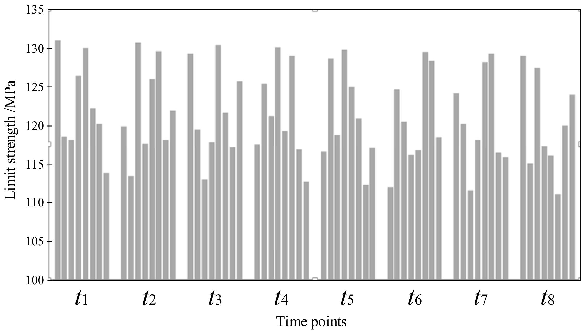
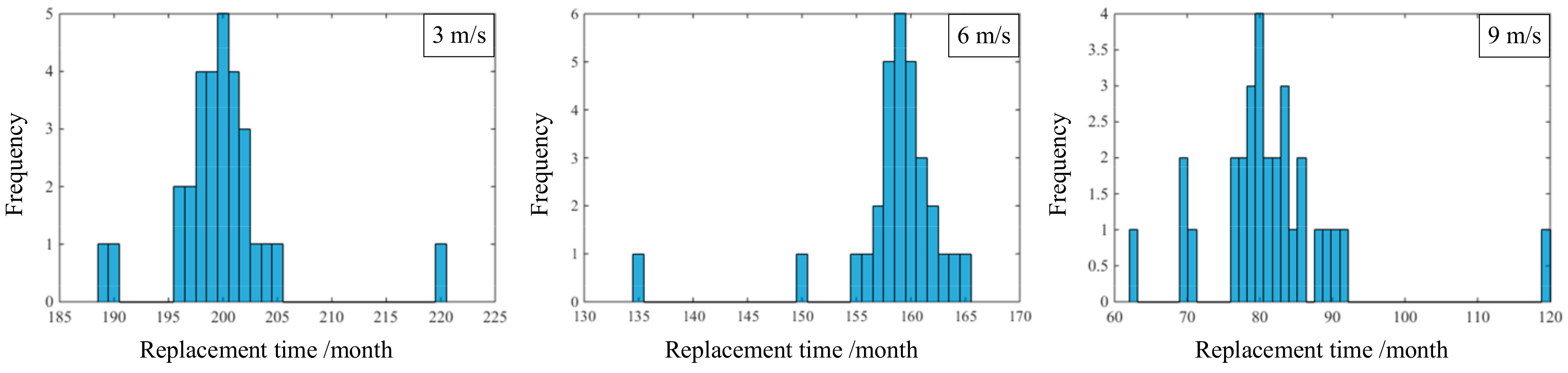
3.2. Experiment Results
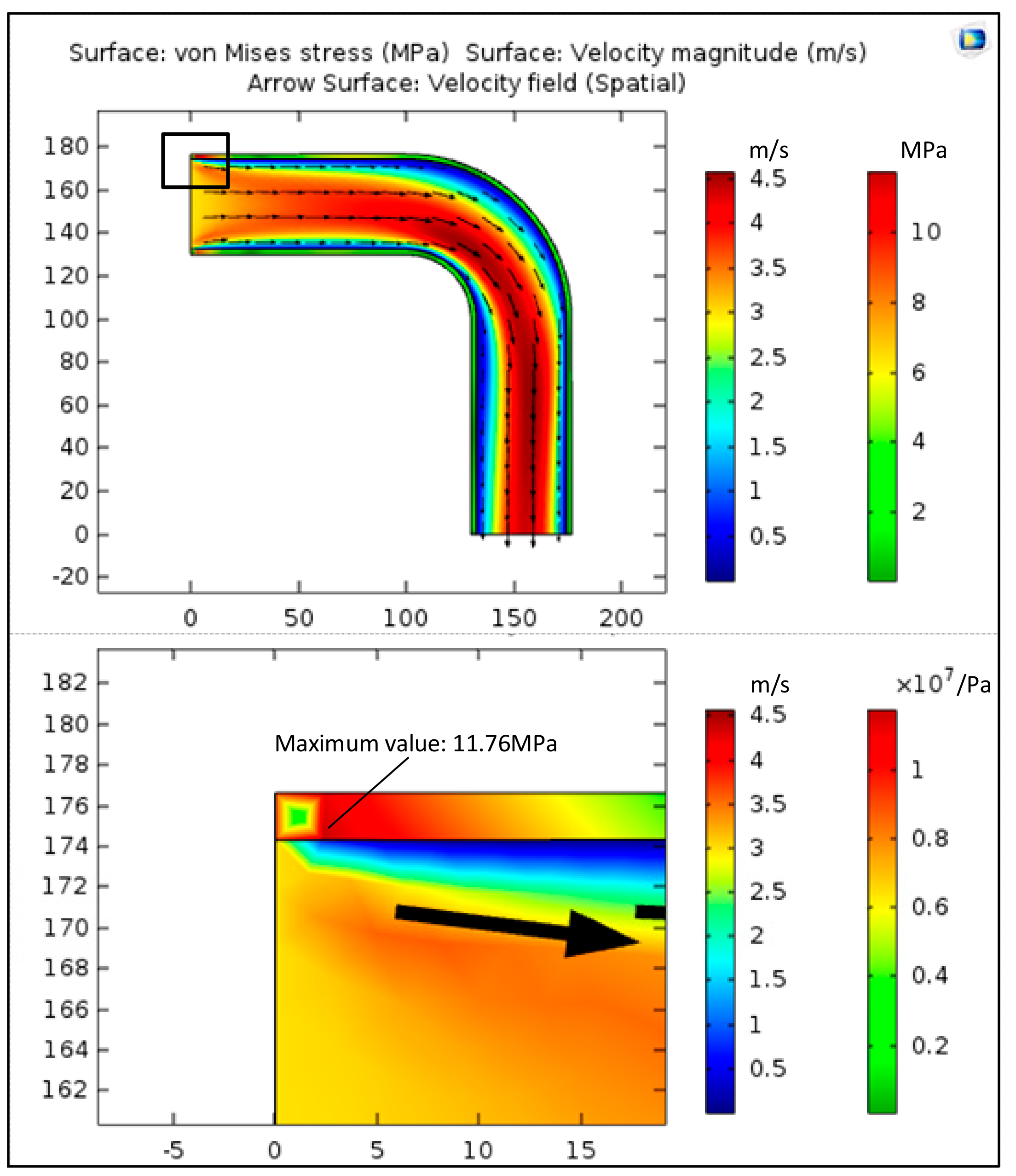
3.3. Stress Simulation Analysis
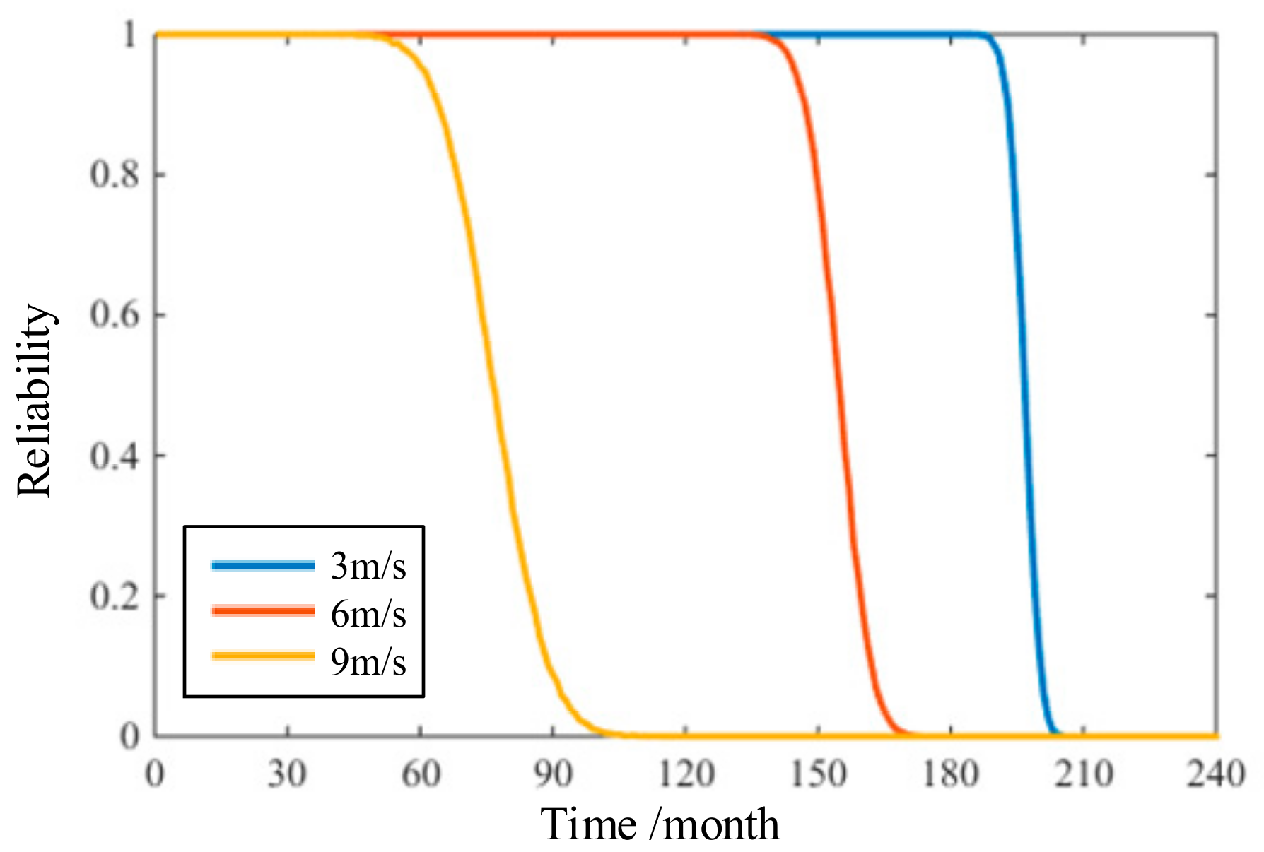
3.4. Reliability Analysis
4. Discussion
4.1. Compared with Traditional Method
4.2. Verifying the Accuracy of Two Methods by Maintenance Records
5. Conclusions
- (1)
- During the degradation process, using the relationship of characteristic parameters over time to represent the stochastic degradation process, the randomness at any time can be easily and accurately described. Based on this, the stochastic degradation process of copper bending pipe is the PDF which contains a function over time, and the reliability curve can be calculated by interference theory.
- (2)
- The life of copper bending pipe calculated by the method proposed in this paper and the life calculated by the traditional method were different by nearly two times. Comparing the maintenance records, it is more accurate and secure to obtain the replacement cycle of copper bending pipe by choosing 0.5 as the reliability indicator of the method in this paper.
- (3)
- The mathematical model which was used to describe the degradation of copper bending pipe can also be used to model the degradation process of other materials due to the widespread occurrence of randomness and multiplicity.
- (4)
- This paper proposes a kind of Monte Carlo method to solve the random distribution over time. At any time, by comparing the pseudorandom from two PDFs and recording the number of times that the limit strength is larger than the maximum stress, the reliability is the ratio of these records.
Acknowledgments
Author Contributions
Conflicts of Interest
Appendix A

References
- Tuck, C.D.S.; Powell, C.A.; Nuttall, J. Shreir’s Corrosion; Elsevier: Amsteldam, The Netherlands, 2010; pp. 1931–1973. ISBN 9780444527875. [Google Scholar]
- Nunez, L.; Reguera, E.; Corvo, F.; Gonzalez, E.; Vazquez, C. Corrosion of copper in seawater and its aerosols in a tropical island. Corros. Sci. 2005, 47, 461–484. [Google Scholar] [CrossRef]
- Ferreira, J.P.; Rodrigues, J.A.; da Fonseca, I.T.E. Copper corrosion in buffered and non-buffered synthetic seawater: A comparative study. J. Solid State Electrochem. 2004, 8, 260–271. [Google Scholar] [CrossRef]
- Féron, D. Corrosion Behaviour and Protection of Copper and Aluminium Alloys in Seawater; Woodhead Publishing Limited: Cambridge, UK, 2007; pp. 19–44. ISBN 9781845692414. [Google Scholar]
- Sun, B.; Ye, T.Y.; Feng, Q.; Yao, J.H.; Wei, M.M. Accelerated degradation test and predictive failure analysis of B10 copper-nickel alloy under marine environmental conditions. Materials 2015, 8, 6029–6042. [Google Scholar] [CrossRef] [PubMed]
- Kang, D.H.; Kim, S.H.; Lee, C.H.; Lee, J.K.; Kim, T.W. Corrosion fatigue behaviors of HSB800 and its HAZs in air and seawater environments. Mater. Sci. and Eng. A 2013, 559, 751–758. [Google Scholar] [CrossRef]
- Lin, L.Y.; Liu, Z.C.; Zhao, Y.H.; Xu, J. Study on marine corrosion and antifouling behavior of copper alloys exposed to sea areas in China. Rare Metals 2000, 19, 96–100. Available online: http://www.docin.com/p-1486146650.html (accessed on 28 February 2018).
- Hodgkiess, T.; Vassiliou, G. Complexities in the erosion corrosion of copper-nickel alloys in saline water. Desalination 2005, 183, 235–247. [Google Scholar] [CrossRef]
- Saha, D.; Pandya, A.; Singh, J.K. Role of environmental particulate matters on corrosion of copper. Atmos. Pollut. Res. 2016, 7, 1037–1042. [Google Scholar] [CrossRef]
- Sun, F.L.; Ren, S.; Li, Z.; Liu, Z.Y.; Li, X.G.; Du, C.W. Comparative study on the stress corrosion cracking of X70 pipeline steel in simulated shallow and deep sea environments. Mater. Sci. Eng. A 2017, 685, 145–153. [Google Scholar] [CrossRef]
- Ossai, C.I.; Boswell, B.; Davies, I.J. Pipeline failures in corrosive environments—A conceptual analysis of trends and effects. Eng. Failure Anal. 2015, 53, 36–58. [Google Scholar] [CrossRef]
- Velazquez, J.C.; Cruz-Ramirez, J.C.; Valor, A. Modeling localized corrosion of pipeline steels in oilfield produced water environments. Eng. Failure Anal. 2017, 79, 216–231. [Google Scholar] [CrossRef]
- Song, X.G.; Zhai, Z.J.; Zhu, P.C.; Han, J. A stochastic computational approach for the analysis of fuzzy systems. IEEE Access 2017, 5, 13465–13477. [Google Scholar] [CrossRef]
- Vale, C.; Lurdes, S.M. Stochastic model for the geometrical rail track degradation process in the Portuguese railway Northern Line. Reliab. Eng. Syst. Saf. 2013, 116, 91–98. [Google Scholar] [CrossRef]
- Takano, N.; Takizawa, H.; Wen, P.; Odaka, K.; Matsunaga, S.; Abe, S. Stochastic prediction of apparent compressive stiffness of selective laser sintered lattice structure with geometrical imperfection and uncertainty in material property. Int. J. Mech. Sci. 2017, 134, 347–356. [Google Scholar] [CrossRef]
- Fang, S.E.; Ren, W.X.; Perera, R. A stochastic model updating method for parameter variability quantification based on response surface models and Monte Carlo simulation. Mech. Syst. Signal Process. 2012, 33, 83–96. [Google Scholar] [CrossRef] [Green Version]
- Bao, N.; Wang, C.J. A Monte Carlo simulation based inverse propagation method for stochastic model updating. Mech. Syst. Signal Process. 2015, 60, 928–944. [Google Scholar] [CrossRef]
- Deng, Y.; Barros, A.; Grall, A. Degradation modeling based on a time-dependent Ornsteon-Uhlenbeck process and residual useful lifetime estimation. IEEE Trans. Reliab. 2016, 65, 126–140. [Google Scholar] [CrossRef]
- Zhang, Z.X.; Hu, C.H.; Si, X.S. Stochastic degradation process modeling and remaining useful life estimation with flexible random-effects. J. Franklin Inst. 2017, 354, 2477–2499. [Google Scholar] [CrossRef]
- Gebraeel, N.Z.; Lawley, M.A. A neural network degradation model for computing and updating residual life distributions. IEEE Trans. Autom. Sci. Eng. 2008, 5, 154–163. [Google Scholar] [CrossRef]
- Larin, O.; Barkanov, E.; Vodka, O. Prediction of reliability of the corroded pipeline considering randomness of corrosion damage and its stochastic growth. Eng. Failure Anal. 2016, 66, 60–71. [Google Scholar] [CrossRef]
- Li, L.; Liu, M.; Shen, W.M.; Cheng, G.Q. An expert knowledge-based dynamic maintenance task assignment model using discrete stress-strength interference theory. Knowl.-Based Syst. 2017, 131, 135–148. [Google Scholar] [CrossRef]
- Jiang, C.; Huang, X.P.; Han, X.; Zhang, D.Q. A time-variant reliability analysis method based on stochastic process discretization. J. Mech. Des. 2014, 136, 091009. [Google Scholar] [CrossRef]
- Jiang, C.; Huang, X.P.; Wei, X.P.; Liu, N.Y. A time-variant reliability analysis method for structural systems based on stochastic process discretization. Int. J. Mech. Mater. Des. 2017, 13, 173–193. [Google Scholar] [CrossRef]
- Wang, Z.Q.; Chen, W. Time-variant reliability assessment through equivalent stochastic process transformation. Reliab. Eng. Syst. Saf. 2016, 152, 166–175. [Google Scholar] [CrossRef]
- Drach, A.; Tsukrov, I.; DeCew, J. Field studies of corrosion behaviour of copper alloys in natural seawater. Corros. Sci. 2013, 76, 453–464. [Google Scholar] [CrossRef]
- Bautista, B.E.T.; Wikiel, A.J.; Datsenko, I. Influence of extracellular polymeric substances (EPS) from Pseudomonas NCIMB 2021 on the corrosion behaviour of 70Cu-30No alloy in seawater. J. Electroanal. Chem. 2015, 737, 184–197. [Google Scholar] [CrossRef]
- Li, S.J.; Zhou, C.Y.; Li, J. Effect of bend angle on plastic limit loads of pipe bends under different load conditions. Int. J. Mech. Sci. 2017, 131–132, 572–585. [Google Scholar] [CrossRef]
- Huang, W.; Askin, R.G. A generalized SSI reliability model considering stochastic loading and strength aging degradation. IEEE Trans. Reliab. 2004, 53, 77–82. [Google Scholar] [CrossRef]
- Mark, G.S.; David, V.R. Time-dependent reliability of deteriorating reinforced concrete bridge decks. Struct. Saf. 1998, 20, 91–109. [Google Scholar] [CrossRef]
- Liao, B.P.; Sun, B.; Yan, M.C.; Ren, Y.; Zhang, W.F.; Zhou, K. Time-variant reliability analysis for rubber O-ring seal considering both material degradation and random load. Materials 2017, 10, 1211. [Google Scholar] [CrossRef] [PubMed]
- Jiao, N.; Guo, J.J.; Liu, S.L. Hydro-pneumatic suspension system hybrid reliability modeling considering the temperature influence. IEEE Access 2017, 5, 19144–19153. [Google Scholar] [CrossRef]
- Wang, H.W.; Xu, T.X.; Mi, Q.L. Lifetime prediction based on Gamma processes from accelerated degradation data. Chin. J. Aeronautics 2015, 28, 172–179. [Google Scholar] [CrossRef]
- Malfliet, A.; Lotfian, S.; Scheunis, L. Degradation mechanisms and use of refractory linings in copper production processes: A critical review. J. Eur. Ceram. Soc. 2014, 34, 849–876. [Google Scholar] [CrossRef]
- Gonzalez-Gonzalez, D.S.; Alejo, R.J.P.; Cantu-Sifuentes, M. A non-linear fuzzy regression for estimating reliability in a degradation process. Appl. Soft Comput. 2014, 16, 137–147. [Google Scholar] [CrossRef]


| Type | Parameters | Value |
|---|---|---|
| Experiment | Experiment period | 24 months |
| Experiment interval | 3 months | |
| Seawater | Density | 1025 |
| Dynamic viscosity | 0.8937 | |
| Copper material | Density | 8960 |
| Young’s modulus | ||
| Poisson’s ratio | 0.35 | |
| Loads | Fluid velocity | 3 , 6 , 9 |
| No. | /Month | ||
|---|---|---|---|
| 1 | 3 | 464.3188 | 0.2638 |
| 2 | 6 | 458.8756 | 0.2661 |
| 3 | 9 | 451.8773 | 0.2695 |
| 4 | 12 | 446.1352 | 0.2722 |
| 5 | 15 | 440.3274 | 0.2750 |
| 6 | 18 | 436.2393 | 0.2768 |
| 7 | 21 | 429.5355 | 0.2803 |
| 8 | 24 | 413.1314 | 0.2903 |
| No. | /Month | ||
|---|---|---|---|
| 1 | 3 | 2.2976 | 0.0008 |
| 2 | 6 | 2.2872 | 0.0015 |
| 3 | 9 | 2.2827 | 0.0023 |
| 4 | 12 | 2.2763 | 0.0031 |
| 5 | 15 | 2.2748 | 0.0033 |
| 6 | 18 | 2.2653 | 0.0047 |
| 7 | 21 | 2.2569 | 0.0051 |
| 8 | 24 | 2.2513 | 0.0058 |
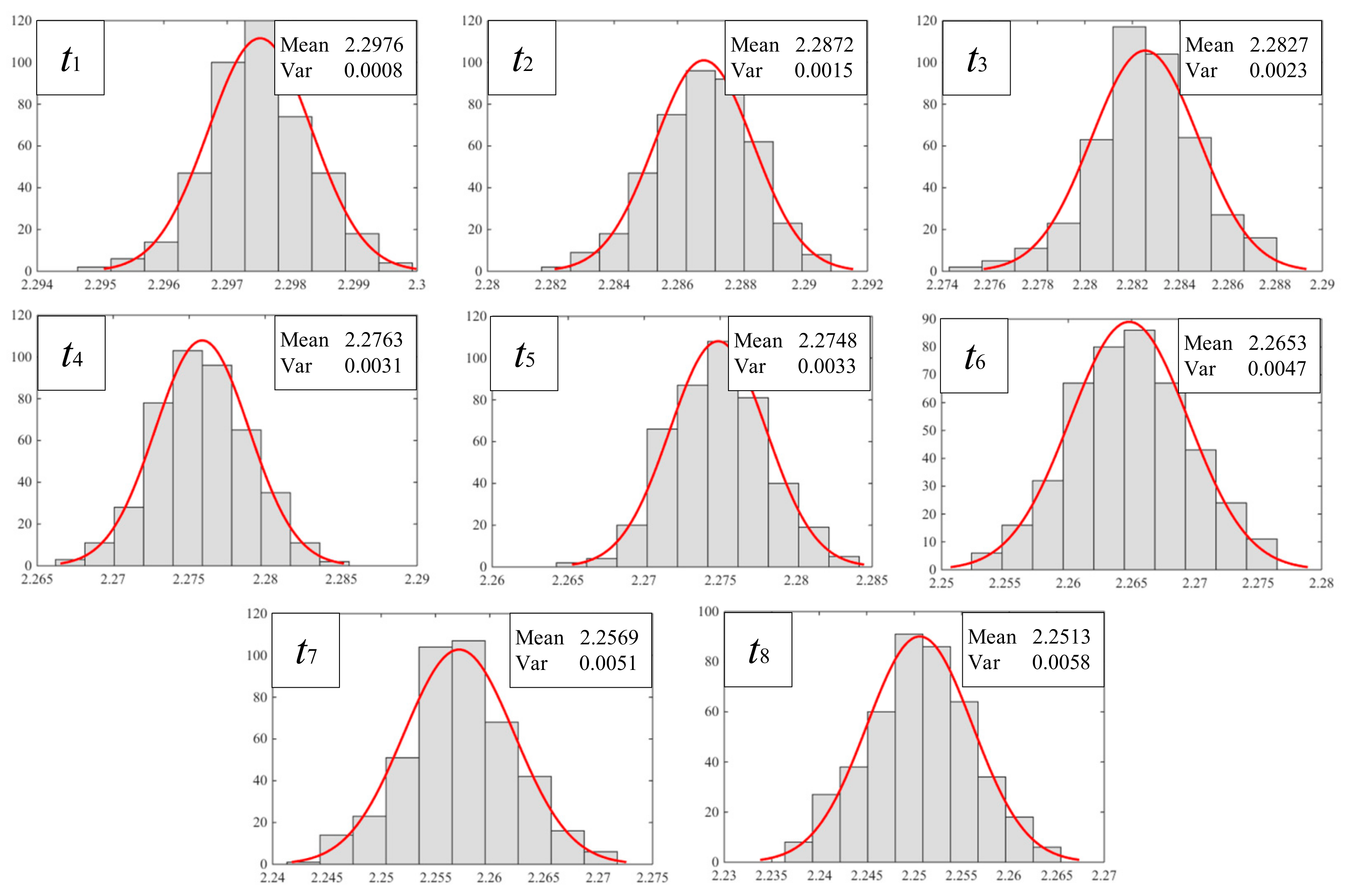
| No. | /Month | ||
|---|---|---|---|
| 1 | 3 | 2.2976 | 0.0008 |
| 2 | 6 | 2.2872 | 0.0015 |
| 3 | 9 | 2.2827 | 0.0023 |
| 4 | 12 | 2.2763 | 0.0031 |
| 5 | 15 | 2.2748 | 0.0033 |
| 6 | 18 | 2.2653 | 0.0047 |
| 7 | 21 | 2.2569 | 0.0051 |
| 8 | 24 | 2.2513 | 0.0058 |
| Flow Velocity | Type | Complete Failure | Corresponding Reliability in This Paper |
|---|---|---|---|
| 3 m/s | Traditional | 506 months | 0 |
| This paper | 208 months | - | |
| 6 m/s | Traditional | 142 months | 0.9732 |
| This paper | 175 months | - | |
| 9 m/s | Traditional | 45 months | 0.9986 |
| This paper | 121 months | - |
© 2018 by the authors. Licensee MDPI, Basel, Switzerland. This article is an open access article distributed under the terms and conditions of the Creative Commons Attribution (CC BY) license (http://creativecommons.org/licenses/by/4.0/).
Share and Cite
Sun, B.; Liao, B.; Li, M.; Ren, Y.; Feng, Q.; Yang, D. A Time-Variant Reliability Model for Copper Bending Pipe under Seawater-Active Corrosion Based on the Stochastic Degradation Process. Materials 2018, 11, 507. https://doi.org/10.3390/ma11040507
Sun B, Liao B, Li M, Ren Y, Feng Q, Yang D. A Time-Variant Reliability Model for Copper Bending Pipe under Seawater-Active Corrosion Based on the Stochastic Degradation Process. Materials. 2018; 11(4):507. https://doi.org/10.3390/ma11040507
Chicago/Turabian StyleSun, Bo, Baopeng Liao, Mengmeng Li, Yi Ren, Qiang Feng, and Dezhen Yang. 2018. "A Time-Variant Reliability Model for Copper Bending Pipe under Seawater-Active Corrosion Based on the Stochastic Degradation Process" Materials 11, no. 4: 507. https://doi.org/10.3390/ma11040507