Article

Model of the Magnetostrictive Hysteresis Loop with Local Maximum

Institute of Metrology and Biomedical Engineering, Warsaw University of Technology, 02-525 Warsaw, Poland
Materials 2019, 12(1), 105; https://doi.org/10.3390/ma12010105
Submission received: 6 December 2018 / Revised: 20 December 2018 / Accepted: 26 December 2018 / Published: 30 December 2018
(This article belongs to the Collection Magnetoelastic Materials)

Abstract

:
This paper presents a model of the magnetostrictive hysteresis loop with local maximum. The model is based on the differential equations describing magnetostriction due to the domain wall movement as well as domain magnetization rotation. The transition between these mechanisms of magnetization is quantified by the Maxwell–Boltzmann distribution. Moreover, the lift-off phenomenon in the magnetostrictive hysteresis loop is considered. The proposed model was validated on the results of measurements of magnetostrictive hysteresis loops of Mn0.70Zn0.24Fe2.06O4 ferrite for power application and 13CrMo4-5 construction steel. The results of modeling confirm that the proposed model corresponds well with experimental results. Good agreement was confirmed by determination coefficient R2, which exceeded 0.995 and 0.985 for Mn0.70Zn0.24Fe2.06O4 ferrite for power application and 13CrMo4-5 construction steel, respectively.

1. Introduction

The magnetostriction phenomenon is connected with the changes of the linear dimensions of the sample during the magnetization process. The magnetostrictive phenomenon has great technical importance. It can be used in the development of specialized position [1] and level sensors [2], MEMS (Micro-Electro-Mechanical Systems) sensors [3], as well as ultrasonic transducers [4] and high accuracy actuators [5].
In spite of the fact that magnetostriction has been known for over one hundred years, as well as the great effort that has been taken to understand it, until now a complete quantitative model of the magnetostrictive hysteresis loop has not been presented. However, it is obvious that magnetostrictive characteristics of soft magnetic materials plays a key role in understanding other magnetomechanical effects, such as the Villari effect [6], the Wiedemann effect [7], or the stress dependence of giant magnetoimpedance phenomenon [8], as well as the Matteucci effect [9].
Previously presented research clearly indicates that magnetostriction (λ) is mostly determined by a parabola-shaped curve with the value of magnetization (M) of the material (which may be estimated by the flux density (B)) [10]. Another important approach was the use of hyperbolic Bessel functions, proposed by Sablik [11]. However, proposed solutions are suitable for parabola-shaped λ(B) curves only. It should be stressed that alarge number of soft magnetic materials, such as some Mn-Zn ferrites [12] or constructional steels [13,14], exhibit local maxima on the λ(B) dependence, which makes parabola-shaped models unsuitable for the modeling of magnetostrictive hysteresis loops of such materials.
This paper fills the gap in the state of the art, presenting a quantitative model of the magnetostrictive λ(B) hysteresis loop with local maximum. The presented model considers the transition from the domain wall movement to the domain rotations, causing the changes of the sign of magnetostriction curve derivative. As a result, the proposed model may be used for both the technical development of magnetostrictive sensors and actuators, as well as for physical analyses of magneto-mechanical processes in soft magnetic materials.

2. Principles of Modeling the Magnetostrictive Hysteresis Loops

Magnetostriction in soft magnetic materials is caused by the changes of the total free magneto-mechanical energy of the material sample due to the transition from the paramagnetic to ferromagnetic state, during the cooling of the material and overturning of the Curie temperature. On the basis of magneto-crystalline anisotropy analyses, it may be stated that the dependence of magnetostriction (λ) on the magnetization (M) of magnetic material may be described by the fourth order polynomial [15]:
λ ( M ) = a 1 M 2 + a 2 M 4
This dependence is commonly reduced to the second order polynomial [16]:
λ ( M ) = 3 2 λ s M s 2 M 2
where λs is the saturation magnetostriction and Ms is saturation magnetization. In the case of soft magnetic materials, where relative permeability μr >> 1, Equation (2) may be presented as [17]:
λ ( B ) = 3 2 λ s B s 2 B 2
where B and Bs are flux density in the material and saturation flux density of the material, respectively. Such form of magnetostrictive characteristic model is more convenient for technical applications. For this reason, Equation (3) was successfully used for the technical modeling of magnetostrictive actuators, especially with cores made of giant magnetostrictive materials, such as Terfenol-D [18,19].
On the other hand, analysis of experimental results of measurements of λ(B) hysteresis loop clearly indicates that accurate modeling of these characteristics requires consideration of λ(B) hysteresis (which is different than B(H) hysteresis), as well as the so called “lift-off” phenomenon. The “lift-off” phenomenon is connected with the fact that, during the magnetization loop, magnetostriction never comes back to the value observed in the demagnetized state.
The physical origins of hysteresis on the λ(B) relation are connected with the interaction between residual stresses and magnetostrictive strain. In previous research, it was connected with the hysteretic magnetization equal to the difference between total magnetization (M) and anhysteretic magnetization (Man) [20]. Another approach to this hysteresis was based on the hyperbolic Bessel functions [11], connecting the magnetostriction with the efficient magnetizing field (He) in the magnetic material equal:
H e = H + α M
where H is the magnetizing field, whereas α is the interdomain coupling accordingly to the Bloch theory.
The “lift-off” phenomenon is connected with the fact that, during the magnetization process, the λ(B) characteristic never returns to zero [20]. The physical origins of this effect are not clearly explained; however, it has been observed in experimental measurements of the magnetostrictive hysteresis loops λ(B) and λ(H) of most ferromagnetic materials [11,20,21,22,23,24]. Known previous approaches to quantitative modeling of the “lift-off” phenomenon were focused on the reproduction of the shape of magnetostrictive hysteresis loops considering this phenomenon [20].
The most important problem connected with modeling the magnetostrictive hysteresis loops λ(B) and λ(H) is the fact, in the case of some soft magnetic materials, that local maxima occurs on these dependences. This local maxima was observed in experimental results [12,14,25,26,27]; however, the quantitative model of such a magnetostrictive hysteresis loop was never presented before. Lack of such a model is the significant barrier for understanding the physical background of magneto-mechanical effects, as well as for the practical description of the behavior of ferromagnetic materials required for, for example, the development of transformers or nondestructive testing of elements made of constructional steels.

3. The Proposed Model of the Magnetostrictive Hysteresis Loop with Local Maxima

The proposed model of the magnetostrictive λ(B) hysteresis loop is based on the fact that the mechanism of the magnetization of ferromagnetic material changes during the magnetization process. For smaller values of magnetizing field, magnetization is connected with the domain walls movements, whereas magnetization in the saturation region is mostly caused by the rotation of domains magnetization [15,16]. As a result, magnetostriction λmov(B) in the domain walls movement region of the magnetic hysteresis loop has a parabola shape [16], and may be described by the following differential equation:
d λ m o v d B = 2 a 1 B
where a1 is the parameter determined in the same way as the parameters in Equation (3). However, for the domain rotations region, the magnetostriction λrot is connected mostly with the rotation from the easy axis to hard axis. As a result, the linear dependence of λrot(B) may be observed in this area [28], represented by the following differential equation:
d λ r o t d B = a 2
where a2 is the parameter describing the slope of the magnetostrictive curve in the saturation region. The transition between the magnetization mechanisms based on the domain wall movement and domain magnetization rotation may be quantified by the Maxwell–Boltzmann statistical distribution, of which the cumulative distribution function is given by the following equation [29]:
W ( B ) = e r f ( B B s w i t c h k 2 ) 2 π ( B B s w i t c h ) e ( B B s w i t c h ) / ( 2 k 2 ) k
where Bswitch is the value of flux density B when the mechanism of magnetization starts to change from domain walls movement to domain magnetization rotation, and k determines the intensity of this process. The so-called error function erf(x), necessary to determine Maxwell­­–Boltzmann statistical distribution, is given by the following equation [29]:
e r f ( x ) = 1 π x x e t 2 d t
Figure 1 presents the example of the magnetic hysteresis B(H) loop together with W(B) dependence. The region of the domain wall movement, the region of the domains magnetization rotation, as well as the region of mixed mechanism can be clearly observed.
Finally, the differential equation determining the flux density B dependence of anhysteretic magnetostriction λanhyst is stated as:
d λ a n h y s t d B = d λ m o v d B ( 1 W ( B ) ) + d λ r o t d B W ( B )
with the initial condition λanhyst(B) = 0 for B = 0.
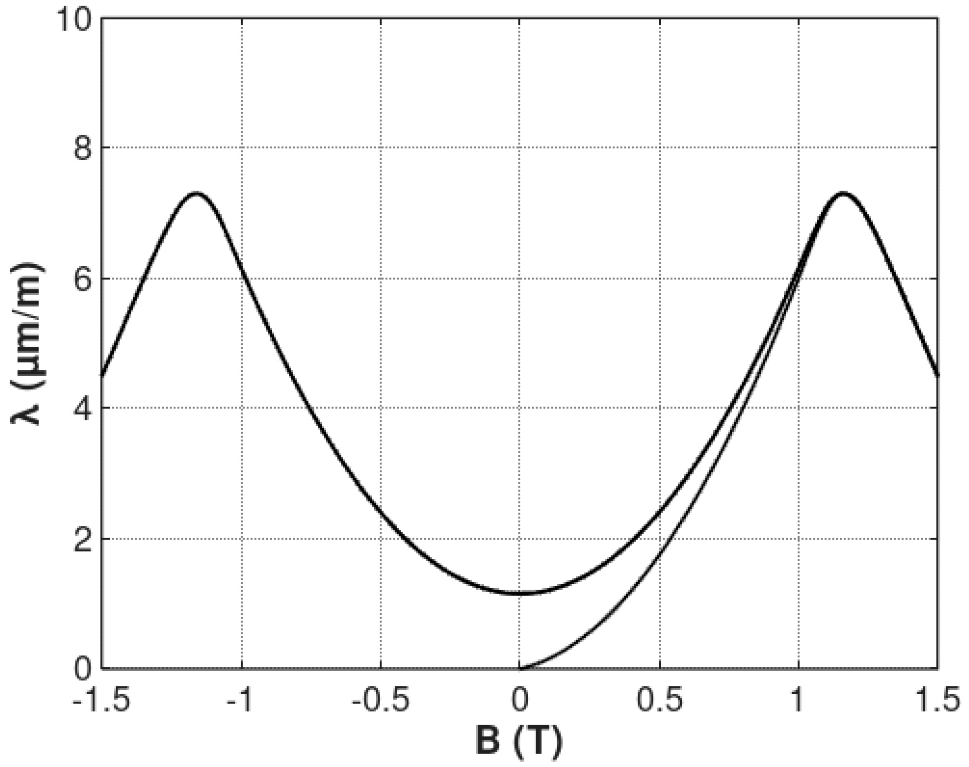
The example of the λanhyst(B) curve stated by Equation (9) is presented in Figure 2. As in the case of real samples, the maximal value of magnetostriction λmax is significantly higher than saturation magnetostriction λs.
The solution proposed to model the “lift-off” phenomenon is similar to the one proposed by Sablik et al. [11,20]. Value of the magnetostriction component λlift-off describing this phenomenon is proportional to flux density B, if the value of flux density B is higher than the value of flux density Bprev reached previously by the material. Otherwise, component λlift-off remains unchanged, as the last reached value. Such mechanism describes the physical background of “lift-off” phenomenon, where the magnetostriction component λlift-off is connected with the interaction of the magnetostriction strain with the residual stresses in the material. The magnetostriction component λlift-off is determined by the following set of differential equations [11]:
d λ l i f t o f f d B = a l i f t o f f   f o r   B > B p r e v d λ l i f t o f f d B =   0   o t h e r w i s e
The example of flux density B dependence of anhysteretic magnetostriction λanhyst considering the “lift-off” phenomenon is presented in Figure 3.
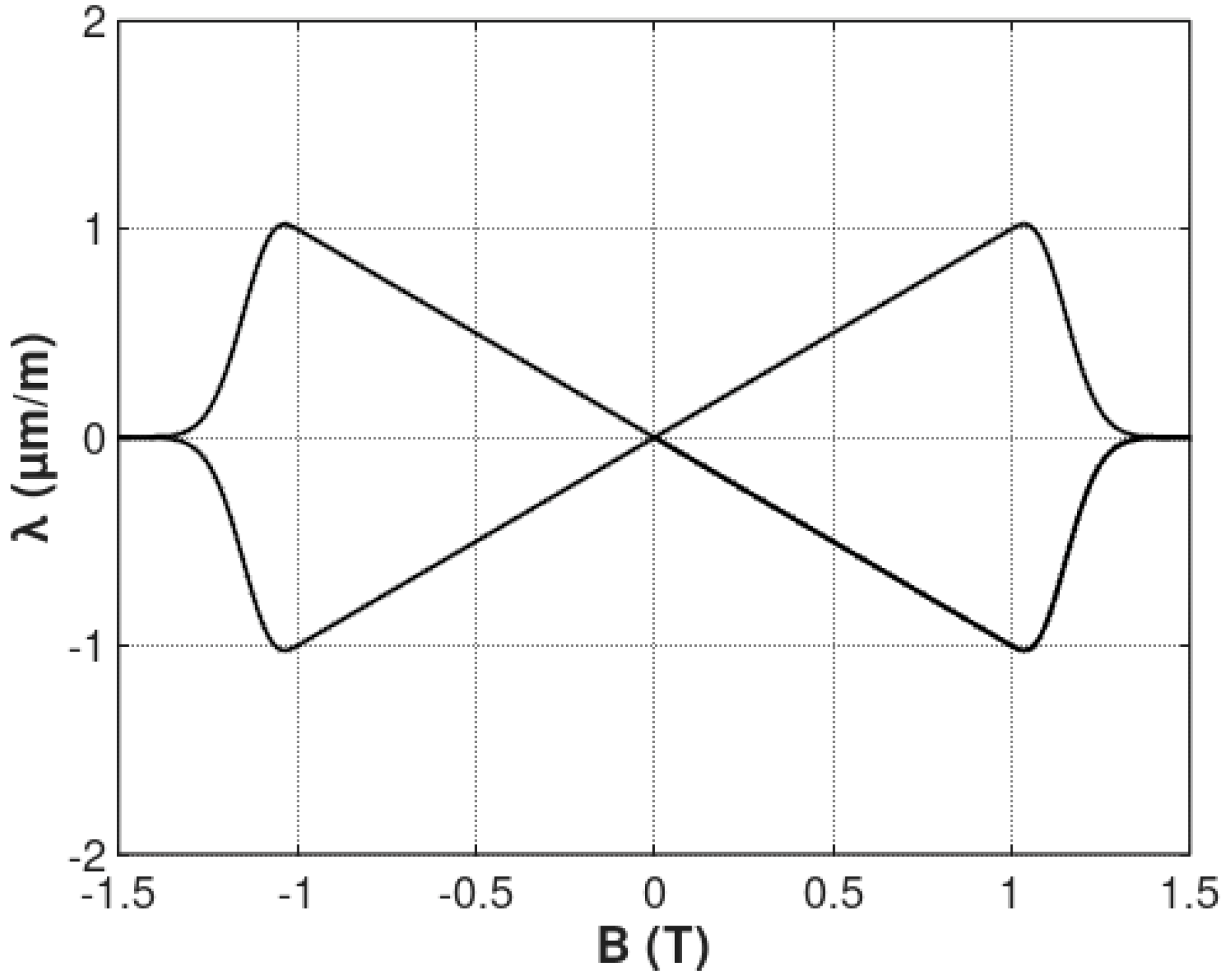
For modelling the hysteretic behavior of magnetostriction λ(B) dependence, it should be highlighted that hysteresis is connected with the domain walls movement magnetization mechanism. Domain magnetization rotation is anhysteretic, which is what can be observed on both B(H) and λ(B) dependencies. As a result, the hysteretic component of the magnetostriction hysteresis loop λhyst can be described as:
λ h y s t ( B ) = ( 1 W ( B ) ) · a h y s t B
where ahyst determines the magnetostrictive hysteresis. The flux density B dependence of magnetostrictive hysteresis λhyst is presented in Figure 4.
Finally, the λ(B) hysteresis loop can be calculated as a sum of the components of magnetostriction:
λ ( B ) = λ a n h y s t ( B ) + λ l i f t o f f ( B ) + λ h y s t ( B )
The example of the magnetostrictive λ(B) hysteresis loop is presented in Figure 5. It can be observed that the shape of the λ(B) hysteresis loop well reflects the shape of such loops presented in the literature.

4. Validation of the Model

4.1. Materials and the Method of Measurements

The proposed model was verified on the basis of experimental measurements of magnetostrictive hysteresis loops of Mn0.70Zn0.24Fe2.06O4 ferrite for power application [12] and 13CrMo4-5 construction steel [14]. Measurements of the magnetostrictive hysteresis loop were carried out on the frame-shaped samples [30] with strain gauges. Semiconductor strain gauges and foil strain gauges were used for the measurements of the samples made of Mn0.70Zn0.24Fe2.06O4 ferrite and 13CrMo4-5 construction steel, respectively. Measurements were performed in room temperature in the quasi-static mode, with the magnetizing field frequency of 0.2 Hz.
A schematic block diagram of the magnetostriction measuring system [12] is presented in Figure 6. Magnetizing winding of the frame-shaped sample was connected to the voltage-current converter BOP36-6M produced by Kepco, USA. The sensing winding as connected to fluxmeter type 480, produced by Lakeshore, USA, enabling real-time measurements of flux density in the core. The strain gauges were connected to a specialized MT-12 bridge, enabling strain gauge sensitivity adjustments. During the measurements, the temperature of the sample was monitored by the thermocouple-based sensor. The whole system was controlled by PC computer, with LabView software equipped in PCI-6221 data acquisition and control card.

4.2. Identification of the Parameters of the Model

The proposed model of the magnetostrictive λ(B) hysteresis loop, stated by Equations (5)–(12), was implemented in Octave 4.4.1, open-source Matlab alternative. For solving the ordinary differential equations, stating the model of themagnetostrictive hysteresis loop, the fourth order Runge–Kutta algorithm was used [31]. Identification of the model’s parameters was carried out on the basis of the minimization process, performed by a derivative-free Nelder and Mead simplex algorithm [32]. The target function G for minimization was determined as the sum of the squared differences between the experimental data and the results of the modeling given by the following equation [33]:
G = i = 1 n ( λ m e a s ( B i ) λ m o d e l ( B i ) ) 2
where λmeas(Bi) is the results of measurements of the magnetostrictive hysteresis loop for the set of given values of flux density Bi; and λmodel(Bi) is the results of the modeling of the magnetostrictive hysteresis loop for the same set of flux density Bi values.
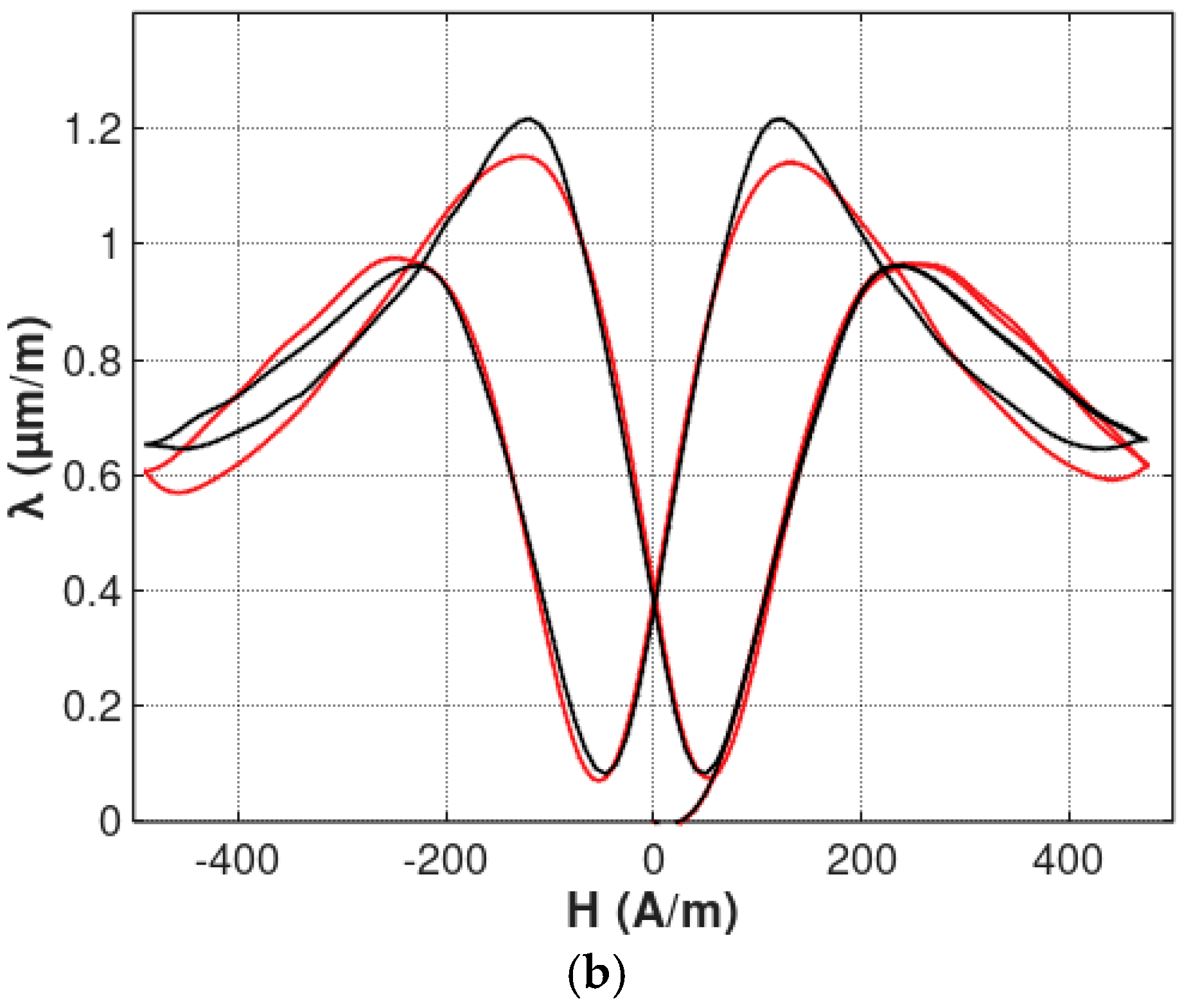
Parameters of the magnetostrictive hysteresis loops of Mn0.70Zn0.24Fe2.06O4 ferrite for power application and 13CrMo4-5 construction steel, identified during the optimization process, are presented in the Table 1. The results of this modeling are presented in Figure 7 and Figure 8 for Mn0.70Zn0.24Fe2.06O4 ferrite, for power application and 13CrMo4-5 construction steel, respectively. Figures present both λ(B) and λ(H) hysteresis loops.
It should be highlighted, that the proposed model very well described the shape of both magnetostrictive λ(B) and λ(H) hysteresis loops. The quality of the model was also confirmed by the value of the R2 determination coefficient, which describes the proportion of the variance described by the model and the variance of the results of measurement. For λ(B) hysteresis loops, the R2 coefficient exceeded 0.995 and 0.985, in the case of Mn0.70Zn0.24Fe2.06O4 ferrite, for power application and 13CrMo4-5 steel, respectively. Such high values of R2 determination coefficients confirms, quantitatively, that the proposed model is suitable for modeling λ(B) and λ(H) magnetostrictive hysteresis loops with local maxima. On the other hand, accuracy of the model for 13CrMo4-5 steel is worse than for Mn0.70Zn0.24Fe2.06O4 ferrite. This effect is probably connected with the fact that the presented model does not consider nucleation and annihilation mechanisms in the sample. These phenomena should be the subject of further research.

5. Conclusions

The presented results of the measurements of both magnetostrictive λ(B) and λ(H) hysteresis loops of Mn0.70Zn0.24Fe2.06O4 ferrite, for power application and steel 13CrMo4-5, confirm that, in the case of these materials, local maxima occur on the magnetostrictive hysteresis loop. To model such a magnetostrictive hysteresis loop the, change of magnetization and magnetostriction mechanisms should be considered.
The proposed model utilizes the cumulative distribution function of Maxwell–Boltzmann statistical distribution to quantify the transition from domain walls movement to domain magnetization rotation. As a result, a new model of the magnetostrictive hysteresis loop was presented, considering previously proposed descriptions of the magnetostrictive hysteresis and magnetostrictive “lift-off” phenomenon. The proposed model very well describes experimental results, efficiently reproducing the maxima on the magnetostrictive λ(B) and λ(H) hysteresis loops. The high quality of the model was confirmed, quantitatively, by the value of the R2 determination coefficient, which exceeded 0.995 and 0.985, for Mn0.70Zn0.24Fe2.06O4 ferrite, for power application and 13CrMo4-5 steel, respectively.
Due to good agreement with the experimental results, the proposed model may be used for works focused on understanding the magnetostrictive phenomena in steels and soft ferrites. In addition, the proposed model may be used for the modeling of the magnetostrictive behavior of inductive components with inductive cores made of soft magnetic materials with non-monotonous magnetostrictive characteristics. Such components are commonly used in power conversion devices, such as switching-mode power supplies.

Funding

This work was fully supported by the statutory funds of the Institute of Metrology and Biomedical Engineering, WUT.

Conflicts of Interest

The author declares no conflict of interest.

References

  1. Seco, F.; Martin, J.M.; Jimenez, A.R. Improving the Accuracy of Magnetostrictive Linear Position Sensors. IEEE Trans. Instrum. Meas. 2009, 58, 722–729. [Google Scholar] [CrossRef]
  2. Li, Y.; Sun, L.; Jin, S.; Sun, L.B. Development of Magnetostriction Sensor for on-line Liquid Level and Density Measurement. In Proceedings of the 6th World Congress on Intelligent Control and Automation, Dalian, China, 21–23 June 2006; pp. 5162–5166. [Google Scholar] [CrossRef]
  3. Chang, H.-C.; Liao, S.-C.; Hsieh, H.-S.; Wen, J.-H.; Lai, C.-H.; Fang, W. Magnetostrictive type inductive sensing pressure sensor. Sens. Actuators A Phys. 2016, 238, 25–36. [Google Scholar] [CrossRef]
  4. Li, P.; Liu, Q.; Li, S.; Wang, Q.; Zhang, D.; Li, Y. Design and numerical simulation of novel giant magnetostrictive ultrasonic transducer. Res. Phys. 2017, 7, 3946–3954. [Google Scholar] [CrossRef]
  5. Zhu, W.; Bian, L.X.; Cheng, L.; Rui, X.T. Non-linear compensation and displacement control of the bias-rate-dependent hysteresis of a magnetostrictive actuator. Precis. Eng. 2017, 50, 107–113. [Google Scholar] [CrossRef]
  6. Bieńkowski, A.; Kulikowski, J. The magneto-elastic Villari effect in ferrites. J. Magn. Magn. Mater. 1980, 19, 120–122. [Google Scholar] [CrossRef]
  7. Li, M.; Li, J.; Bao, X.; Mu, X.; Gao, X. Magnetostrictive Fe82Ga13.5Al4.5 wires with large Wiedemann twist over wide temperature range. Mater. Des. 2017, 135, 197–203. [Google Scholar] [CrossRef]
  8. Zhukov, A.; Ipatov, M.; Churyukanova, M.; Talaat, A.; Blanco, J.M.; Zhukova, V. Trends in optimization of giant magnetoimpedance effect in amorphous and nanocrystalline materials. J. Alloys Compd. 2017, 727, 887–901. [Google Scholar] [CrossRef]
  9. Dimitropoulos, P.D.; Avaritsiotis, J.N. A micro-fluxgate sensor based on the Matteucci effect of amorphous magnetic fibers. Sens. Actuators A Phys. 2001, 94, 165–176. [Google Scholar] [CrossRef]
  10. Dapino, M.J. On magnetostrictive materials and their use in adaptive structures. Struct. Eng. Mech. 2004, 17, 303–329. [Google Scholar] [CrossRef]
  11. Sablik, M.J.; Jiles, D.C. A model for hysteresis in magnetostriction. J. Appl. Phys. 1988, 64, 5402–5404. [Google Scholar] [CrossRef]
  12. Bieńkowski, A.; Szewczyk, R. Magnetostrictive Properties of Mn0.70Zn0.24Fe2.06O4 Ferrite. Materials 2018, 11, 1894. [Google Scholar] [CrossRef] [PubMed]
  13. Juś, A.; Nowak, P.; Gińko, O. Assessment of the Magnetostrictive Properties of the Selected Construction Steel. Acta Phys. Pol. A 2017, 131, 1084–1086. [Google Scholar] [CrossRef]
  14. Gińko, O.; Juś, A.; Szewczyk, R. Test Stand for Measuring Magnetostriction Phenomena Under External Mechanical Stress with Foil Strain Gauges. In Advances in Intelligent Systems and Computing, Proceedings of the Challenges in Automation, Robotics and Measurement Techniques (ICA 2016), Warsaw, Poland, 2–4 March 2016; Szewczyk, R., Zieliński, C., Kaliczyńska, M., Eds.; Springer: Berlin, Germany, 2017. [Google Scholar] [CrossRef]
  15. Bozorth, R.M. Ferromagnetism; Wiley-IEEE Press: New York, NY, USA, 1978. [Google Scholar]
  16. Jiles, D.C. Introduction to Magnetism and Magnetic Materials; CRC Press: Boca Raton, FL, USA, 2015. [Google Scholar]
  17. Calkins, F.T.; Smith, R.C.; Flatau, A.B. Energy-based hysteresis model for magnetostrictive transducers. IEEE Trans. Magn. 2000, 36, 429–439. [Google Scholar] [CrossRef] [Green Version]
  18. Hsu, C.-H.; Huang, Y.-M.; Hsieh, M.-F.; Fu, C.-M.; Adireddy, S.; Chrisey, D.B. Transformer sound level caused by core magnetostriction and winding stress displacement variation. AIP Adv. 2017, 7, 056681. [Google Scholar] [CrossRef] [Green Version]
  19. Cheng, S.-J.; Liu, J.-J.; Chang, Y.-H.; Fu, C.-M.; Hsu, C.-H.; Lee, C.-Y.; Chang, C.-W. Correlation of magnetostriction variation on magnetic loss and noise for power transformer. J. Appl. Phys. 2015, 117, 17E716. [Google Scholar] [CrossRef]
  20. Sablik, M.J.; Jiles, D.C. Coupled magnetoelastic theory of magnetic and magnetostrictive hysteresis. IEEE Trans. Magn. 1993, 29, 2113–2123. [Google Scholar] [CrossRef] [Green Version]
  21. Bieńkowski, A.; Kaczkowski, Z. Major and minor magnetostriction hysteresis loops of Co–Cu–Ni ferrite. J. Magn. Magn. Mater. 2000, 215–216, 234–236. [Google Scholar] [CrossRef]
  22. Szewczyk, R.; Bieńkowski, A.; Kolano-Burian, A. Magnetostrictive properties of Fe40Ni38Mo4B18 alloy. Mater. Sci. Eng. A 2004, 375–377, 1137–1139. [Google Scholar] [CrossRef]
  23. Szewczyk, R. Modelling of the magnetic and magnetostrictive properties of high permeability Mn-Zn ferrites. PRAMANA J. Phys. 2006, 67, 1165–1171. [Google Scholar] [CrossRef]
  24. Ueda, Y.; Takahashi, M. Structure and magnetic properties in single-crystal iron film electrodeposited on a (110) copper crystal. J. Magn. Magn. Mater. 1988, 71, 212–218. [Google Scholar] [CrossRef]
  25. Gou, J.; Liu, X.; Wu, K.; Wang, Y.; Hu, S.; Zhao, H.; Xiao, A.; Ma, T.; Yan, M. Tailoring magnetostriction sign of ferromagnetic composite by increasing magnetic field strength. Appl. Phys. Lett. 2016, 109, 082404. [Google Scholar] [CrossRef]
  26. Bozorth, R.M.; Tilden, E.F.; Williams, A.J. Anisotropy and Magnetostriction of Some Ferrites. Phys. Rev. 1955, 99, 1788. [Google Scholar] [CrossRef]
  27. Piotrowski, L.; Chmielewski, M.; Augustyniak, B. On the correlation between magnetoacoustic emission and magnetostriction dependence on the applied magnetic field. J. Magn. Magn. Mater. 2016, 410, 34–40. [Google Scholar] [CrossRef]
  28. Tremolet, E. Magnetostriction; C.R.C. Press: London, UK, 1992. [Google Scholar]
  29. Mandl, F. Statistical Physics; John Wiley & Sons: Hoboken, NJ, USA, 2008. [Google Scholar]
  30. Bieńkowski, A. Some problems of measurement of magnetostriction in ferrites under stresses. J. Magn. Magn. Mater. 1992, 112, 143–145. [Google Scholar] [CrossRef]
  31. Atkinson, K.A. An Introduction to Numerical Analysis; John Wiley & Sons: Hoboken, NJ, USA, 1989. [Google Scholar]
  32. Nelder, J.A.; Mead, R. A simplex method for function minimization. Comput. J. 1965, 7, 308–313. [Google Scholar] [CrossRef]
  33. Biedrzycki, R.; Jackiewicz, D.; Szewczyk, R. Reliability and Efficiency of Differential Evolution Based Method of Determination of Jiles-Atherton Model Parameters for X30Cr13 Corrosion Resisting Martensitic Steel. J. Autom. Mob. Robot. Intell. Syst. 2014, 8, 63–68. [Google Scholar] [CrossRef]
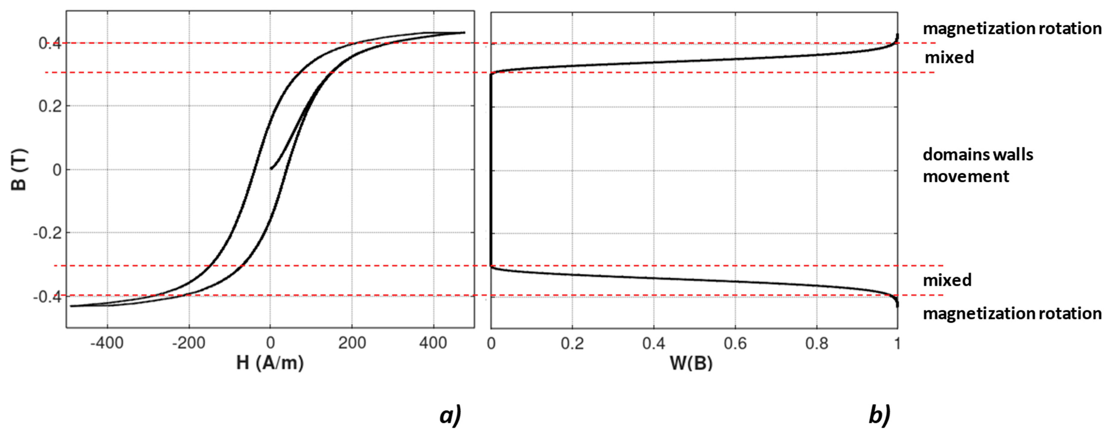
Figure 1. Changes in the mechanism of magnetization in Mn0.70Zn0.24Fe2.06O4 ferrite for power applications: (a) Magnetic hysteresis loop B(H); (b) W(B) dependence determining the mechanism of magnetization.
Materials 12 00105 g001
Figure 2. The flux density B dependence of anhysteretic magnetostriction λanhyst, determined by Equation (9). Parameters: a1 = 5 μ m m 1 T 2 , a2 = 10 μ m m 1 T , Bswitch = 1 T, k = 0.1.
Materials 12 00105 g002
Figure 3. The flux density B dependence of anhysteretic magnetostriction λanhyst considering the “lift-off” phenomenon, calculated for the following parameters: a1 = 5 μ m m 1 T 2 , a2 = 10 μ m m 1 T , Bswitch = 1 T, k = 0.1, alift-off = 1 μ m m 1 T .
Materials 12 00105 g003
Figure 4. The flux density B dependence of magnetostrictive hysteresis λhyst calculated for the following parameters: Bswitch = 1 T, k = 0.1, ahyst = 1 μ m m 1 T .
Materials 12 00105 g004
Figure 5. Magnetostrictive λ(B) hysteresis loop, determined by Equation (12), calculated for the parameters: a1 = 5 μ m m 1 T 2 , a2 = 10 μ m m 1 T , Bswitch = 1 T, k = 0.1, alift-off = 1 μ m m 1 T , ahys = 1 μ m m 1 T .
Materials 12 00105 g005
Figure 6. Schematic diagram of the system used for the measurements of magnetostrictive λ(B) and λ(H), as well as the magnetic B(H) hysteresis loops.
Materials 12 00105 g006
Figure 7. Results of modeling the magnetostrictive hysteresis loops of Mn0.70Zn0.24Fe2.06O4 ferrite for power applications: (a) λ(B) hysteresis loop; (b) λ(H) hysteresis loop. Experimental results—red line; results of modeling—black line.
Materials 12 00105 g007aMaterials 12 00105 g007b
Figure 8. Results of modeling the magnetostrictive hysteresis loops of 13CrMo4-5 steel: (a) λ(B) hysteresis loop; (b) λ(H) hysteresis loop. Experimental results—red line; results of modeling—black line.
Materials 12 00105 g008
Table 1. Parameters of magnetostrictive λ(B) hysteresis loops determined in optimization process.
ParameterUnitMn0.70Zn0.24Fe2.06O4 Ferrite13CrMo4-5 Steel
a1 μ m m 1 T 2 8.106.73
a2 μ m m 1 T −10.07−25.93
BswitchT0.3121.338
k-0.0390.101
alift-off μ m m 1 T 0.2530.495
ahyst μ m m 1 T 0.5610.908
R2-0.9950.985