A Different Approach to Estimate Temperature-Dependent Thermal Properties of Metallic Materials
by

Luís Felipe dos Santos Carollo
, 
Ana Lúcia Fernandes de Lima e Silva
and
Sandro Metrevelle Marcondes de Lima e Silva
* Heat Transfer Laboratory—LabTC, Institute of Mechanical Engineering—IEM, Federal University of Itajubá—UNIFEI, Campus Prof. José Rodrigues Seabra, Av. BPS, 1303, Itajubá 37500-903, MG, Brazil
*
Author to whom correspondence should be addressed.
Materials 2019, 12(16), 2579; https://doi.org/10.3390/ma12162579
Submission received: 19 July 2019
/
Revised: 7 August 2019
/
Accepted: 10 August 2019
/
Published: 13 August 2019
(This article belongs to the Special Issue Thermal Analysis of Materials)
Abstract
:Thermal conductivity, λ, and volumetric heat capacity, ρcp, variables that depend on temperature were simultaneously estimated in a diverse technique applied to AISI 1045 and AISI 304 samples. Two distinctive intensities of heat flux were imposed to provide a more accurate simultaneous estimation in the same experiment. A constant heat flux was imposed on the upper surface of the sample while the temperature was measured on the opposite insulated surface. The sensitivity coefficients were analyzed to provide the thermal property estimation. The Broydon-Fletcher-Goldfarb-Shanno (BFGS) optimization technique was applied to minimize an objective function. The squared difference objective function of the numerical and experimental temperatures was defined considering the error generated by the contact resistance. The temperature was numerically calculated by using the finite difference method. In addition, the reliability of the results was assured by an uncertainty analysis. Results showing a difference lower than 7% were obtained for λ and ρcp, and the uncertainty values were above 5%.
1. Introduction
At present, globalization provides newer, faster, more reliable, and more accurate techniques to estimate thermal properties of materials depending on temperature. The cost of obtaining the parameters is another important issue, since it determines the reliability to compete in the internal and external markets. This paper proposes a technique that may be applied, for example, to accurately select, from the point of view of thermal properties, which materials will be employed in the manufacturing of heat exchangers. The methodology that leads to correct values of the thermal properties allows for saving of energy and other consequent environmental benefits; matters which, recently, have been largely considered. The machining process can be cited as an example for the aforementioned saving. A large amount of heat produced during the cutting process is dissipated to the tool holder. Knowing the values of the thermal conductivity of the tool and the tool holder leads to the correct choice of their material. Therefore, researchers have developed several procedures in this field [1,2].
A number of methods are available to estimate the thermal properties considering precision, speed, and cost, among other characteristics. In this context, Jannot et al. [3] presented a study in which the thermal conductivity of insulated materials was determined based on a pulsed method with a good precision, Xamán et al. [4] applied a guarded hot plate apparatus for the same purpose, and Thomas et al. [5] determined thermal conductivity and specific heat of insulated materials by applying a new experimental design. These thermal properties may be determined individually or together, and a great part of the estimations happen safely, precisely, and rapidly; however, few were used for temperature-dependent estimation or metallic materials. Other researchers present techniques that allow the estimation of only one temperature-dependent thermal property, for example, Aksöz et al. [6] estimated the thermal conductivity of Al-Cu alloys by using a radial heat flow apparatus and changed the initial temperature and Karimi et al. [7] determined the thermal conductivity of silver alloys by varying the temperature based on a linear heat flux apparatus. Recently, many researchers have presented techniques to simultaneously estimate temperature-dependent thermal properties, such as Sadeghi et al. [8] who determined thermal conductivity and diffusivity of SiC samples by applying the microwave heating process, Zamel et al. [9] who presented an improved firework algorithm to solve inverse problems allowing simultaneous estimation of properties of molten salt, and Öztürk et al. [10] who presented a method to estimate thermal conductivity and specific heat temperature-dependent of thermal protective fabric with good results. Other studies were performed [11,12,13,14,15,16], but none of them included the possibility of estimating thermal properties of metals depending on temperature simultaneously. Moreover, the experimental apparatus for most of these techniques is usually expensive.
Thus, this work presents a technique to simultaneously determine volumetric heat capacity, ρcp, and thermal conductivity, λ, of AISI 1045 and AISI 304 samples; variables that depend on temperature. Some advantages of this method are the low cost, the precision, and the speed when compared with the techniques cited. Additionally, the uncertainty analysis presented in this work considers the influence of the numerical and experimental temperature errors and contact resistance. This work presents the betterments carried out concerning Carollo et al. [17].
2. Materials and Methods
2.1. Thermal Design Model
The representation of the one-dimensional (1D) heat diffusion model is presented in Figure 1. This thermal model is obtained by using a resistive heater between two samples, and the sample-heater set is insulated. The thickness of the sample is much smaller than the other dimensions to ensure the one dimension.
The conduction equation for the problem in Figure 1 is:
In accordance with the literature, there are two methods to estimate thermal properties dependent on temperature. In the first method, presented in Özisik [18], the thermal model is based on nonlinear heat conduction. The second method adopts constant thermal properties within a temperature range to solve the thermal model [19]. Thus, the initial temperature was defined (T0) and the estimation of the properties occurred considering 5 °C as the maximum range of temperature. This condition was performed for all the desired temperatures.
Therefore, the heat diffusion equation for the thermal problem with constant thermal properties is expressed as below:
subjected to the following conditions of boundary:
and the initial condition:
where x is the heat direction, t the temporal interval, the applied heat flow, T0 the temperature in the beginning of the process, and L the thickness.
The finite difference method was used to calculate the numerical temperature of the conduction (Equation (2)).
2.2. Objective Function
Equation (6) presents the objective function applied to estimate ρcp and λ:
where m is the number of points where temperature was measured, Y is the measured temperature, is the heater thermal contact resistance, and is the weighted average heat flow.
The optimum values of ρcp and λ are required to minimize Equation (6). To perform this procedure, the BFGS sequential optimization technique [20] is used in this work.
2.3. Experimental Procedure
The experimental apparatus sketch used is shown in Figure 2. As can be seen, all the components are numbered following this configuration: 1: Micro-computer; 2: Data acquisition; 3: Oven; 4: Multimeter; 5: Power supply; and 6: Multimeter.
In this work, two materials were analyzed: AISI 1045 Steel (99.9 × 99.9 × 11.9 mm3) and AISI 304 stainless steel (49.9 × 49.9 × 10.5 mm3). Due to the different dimensions of the samples, a 99.5 × 99.5 × 0.2 mm3 resistive kapton heater with 23.2 Ω was necessary and another of 48.5 × 48.5 × 0.2 mm3 with 24.4 Ω. The resistive kapton heater was chosen due to its thinness, which allows a faster and more uniform warming. An Instrutemp ST-305 D-II power supply (Instrutemp Instrumentos de Medição Ltda, São Paulo, Brazil) was used to provide the adequate heat flow to perform the experiments. To ensure the correct values of current and resistance, calibrated multimeters were used (Minipa ET-2042-C (Minipa do Brasil, Joinvile, Brazil) for the current and Instrutherm MD-380 (Instrutherm Instrumentos de Medição, São Paulo, Brazil) for the resistance. Additionally, a symmetrical assembly was set up to reduce the errors caused by the measurement of heat flux on the top surface. A data acquisition system Agilent 34980A (Agilent, Santa Clara, CA, USA) was used to connect Type T thermocouples (30 AWG), welded by a capacitive discharge. To provide different initial conditions, the heater-sample set was placed inside a MA030 Marconi oven (Marconi Equipamentos para Laboratórios, Piracicaba, Brazil). The whole set was insulated by ceramic fiber plates with two purposes (Figure 1b): To guarantee a 1D heat flow and to reduce the convection effects. Lastly, all the experiments were performed in a temperature-controlled room.
3. Results and Discussion
All the experiments were performed following the procedure defined by Carollo et al. [17].
3.1. AISI 1045 Steel
In order to achieve significant results to simultaneously estimate λ and ρcp, 15 experiments were performed for each initial condition (25 °C, 50 °C, 75 °C, 100 °C, 125 °C, and 150 °C). The experiment lasted 80 s each, following these conditions: 0–10 s with heat flux of 7709 Wm−2; 10–70 s with 1854 Wm−2, and 70–80 s without heat flux. These conditions provide the best estimation of the thermal properties [17] and respect the hypotheses of constant thermal properties for each initial condition, since the difference between the initial and final temperature must be lower than 5 K. Lastly, the temperature was monitored in a time interval of 0.1 s so as to have more data.
To ensure the best region and the ideal condition to determine the thermal properties, two analyses were done: The first analysis corresponded to the sensitivity and objective function and the second concerned the best condition and design for the experiments [17].
Figure 3 presents the sensitivity coefficient (sens. coef.) of ρcp and λ at x = L. These coefficients are important to indicate the best conditions to estimate the properties, such as, experimental time, time interval, number of points analyzed, and others. The sensitivity coefficient of λ increased only in the beginning of the experiment and remained constant after the heat flux was changed, until the power supply was turned off. By analyzing the sensitivity coefficient of ρcp it was possible to confirm that the value increased while there was heat flux. Because of this behavior, the best condition to simultaneously estimate the properties was applying two diverse heat flux intensities, the higher of which was applied in the beginning to maximize the sensitivity for thermal conductivity estimation and the lower was applied to guarantee enough sensitivity for the volumetric heat capacity estimation. It is important to claim that simultaneous estimation was possible because there was no dependence between the sensitivity curves.
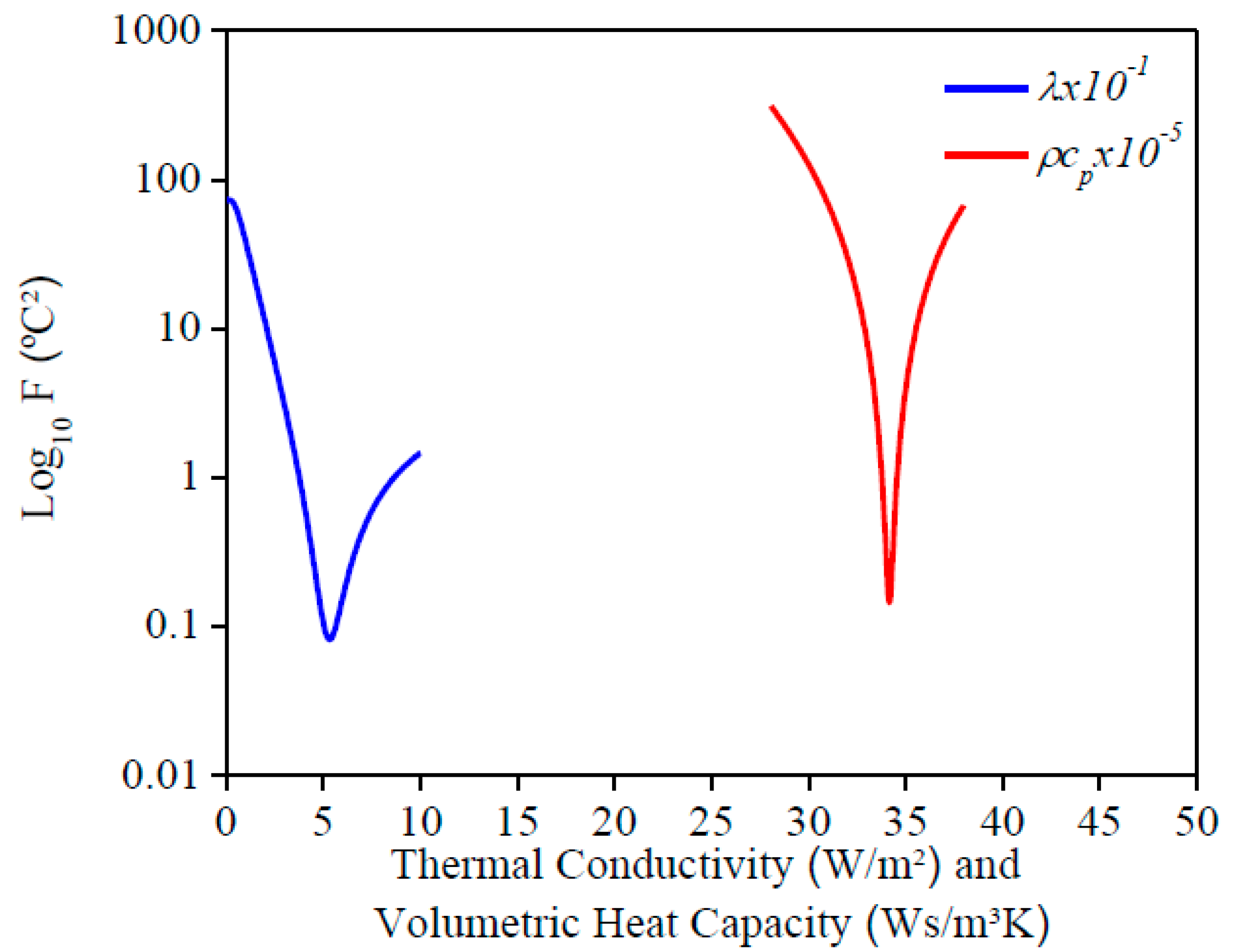
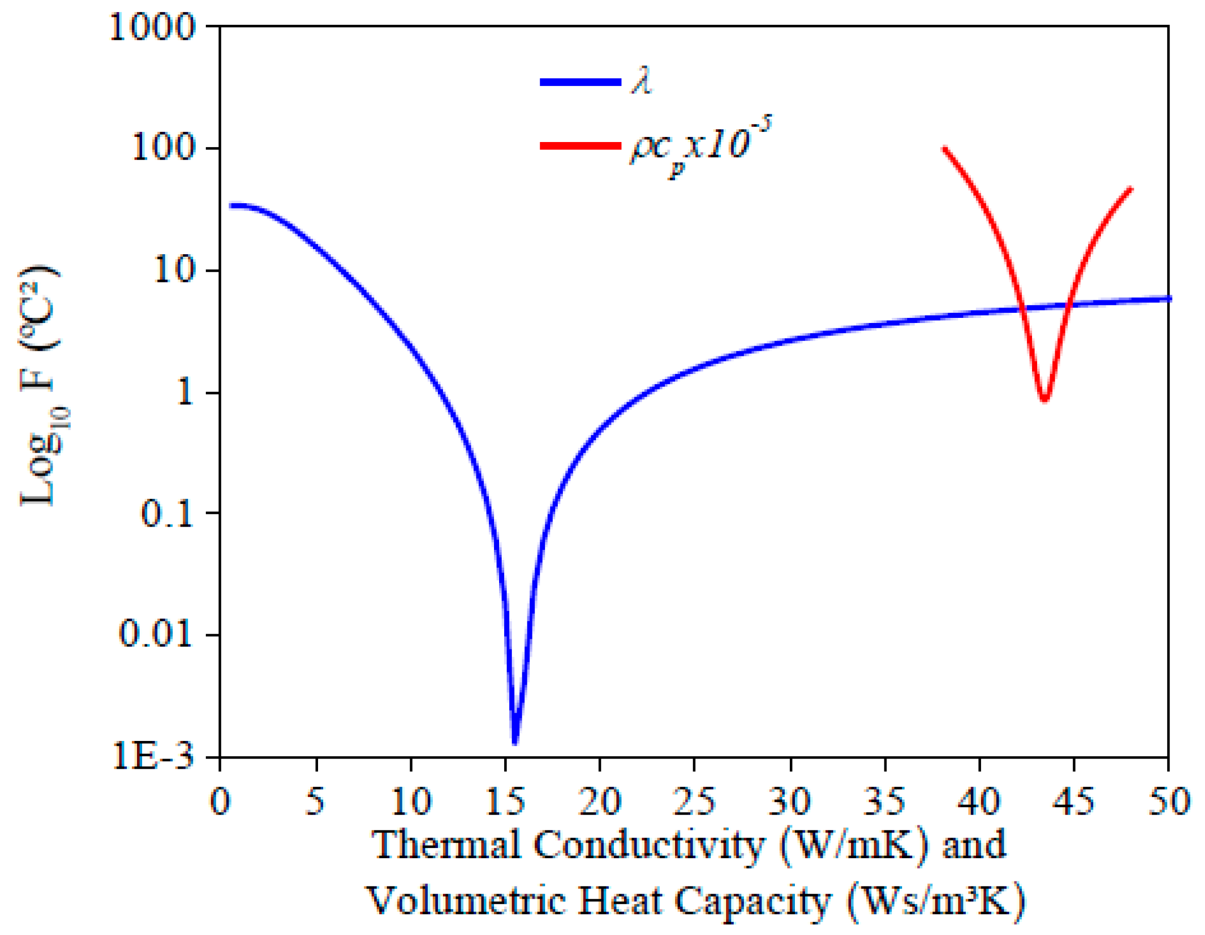
The evaluation of Equation (6) for each property is shown in Figure 4. λ and ρcp were estimated simultaneously due to a minimum value for each property. It is important to inform that the contact resistance of the heater on the sample was considered in Equation (6) to find its influence on the temperature measurements. In this study, a temperature difference of 0.23 °C corresponded to the influence of this contact resistance.
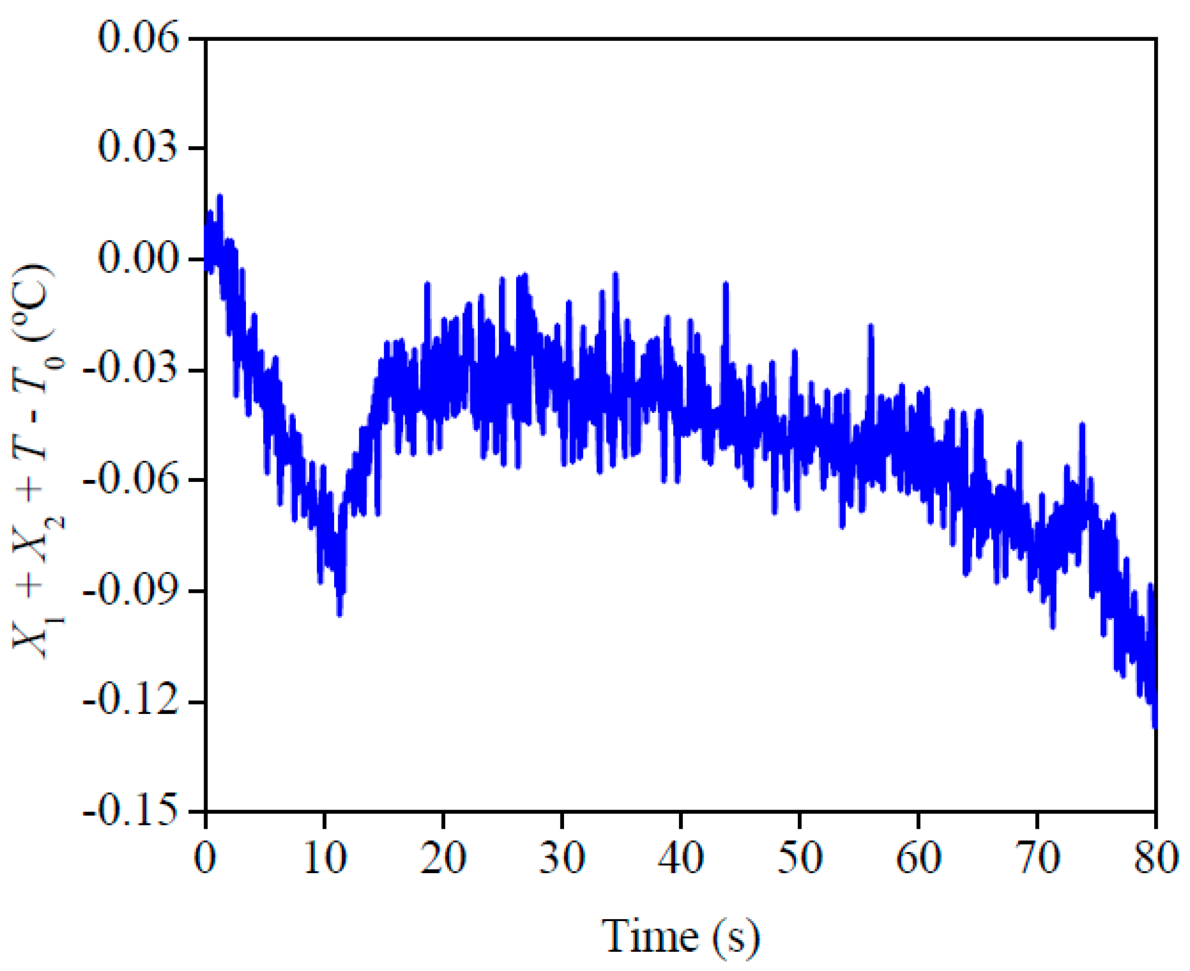
The best condition and design for the experiment is presented in Figure 5. This analysis indicates that the best quality for the experiment was when the sensitivity coefficient of ρcp and λ plus the temperature difference was close to 0 (X1 + X2 + Y − Y0 ≅ 0). This analysis is relevant because it is a complement to the sensitivity analysis, in other words, it is a confirmation that all the established conditions allow a precise property estimation. A good condition of the experiment may be seen here, since the highest difference was around 0.12 °C. This affirmation can be checked when the obtained difference is compared with the difference between the final and initial temperature of each experiment, which is around 4 °C.
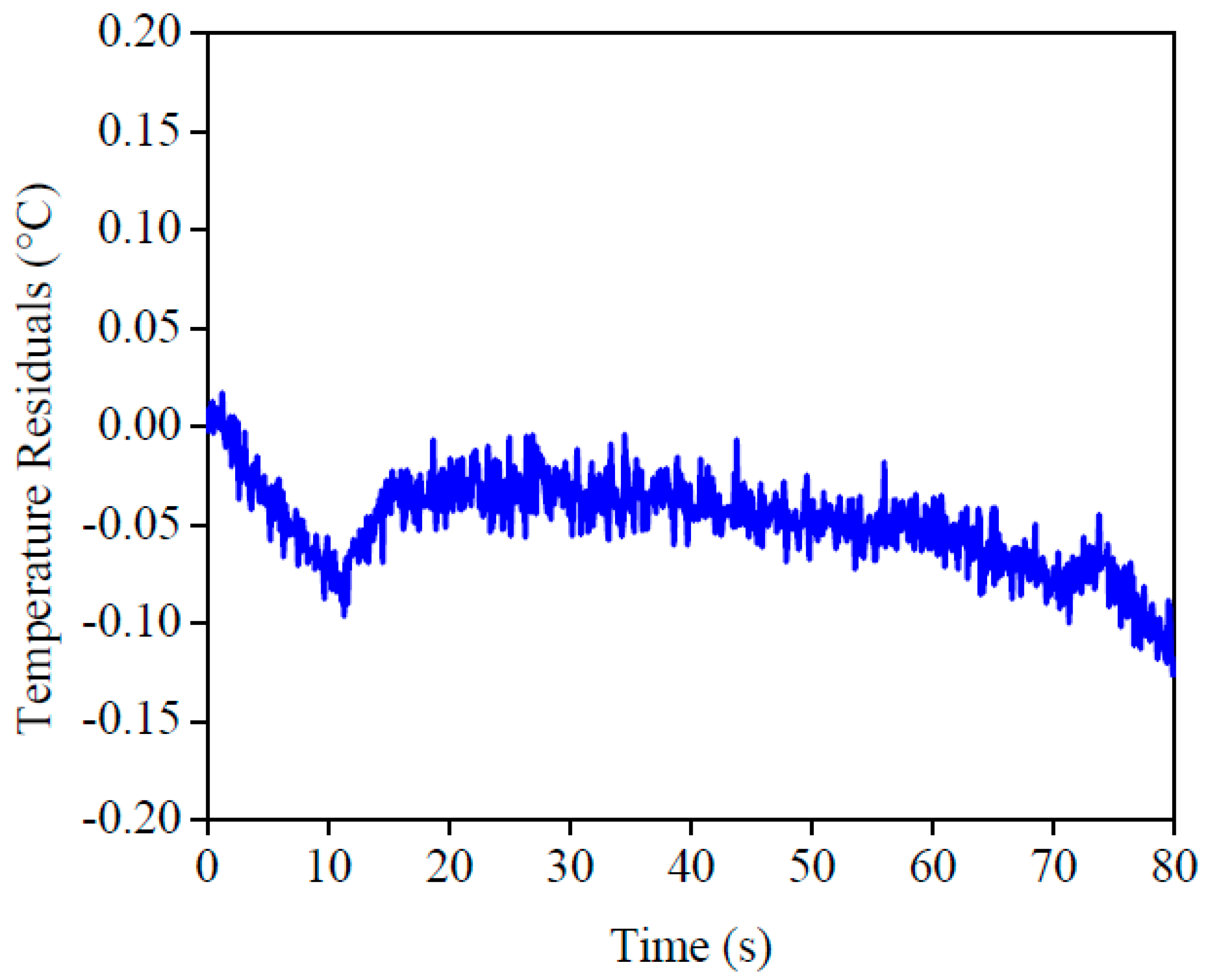
Figure 6 shows the applied heat flux at x = 0 and the temperatures values at x = L. It is possible to see the good agreement between the experimental temperature and numerical temperature, which was calculated by using the obtained thermal properties. To confirm this affirmation, Figure 7 presents the residuals between these temperatures. Once the maximum difference found was around 0.10 °C, it was possible to confirm the good quality of the methodology. This affirmation can be validated by comparing the obtained difference with the thermocouple uncertainty, that it is around 0.10 °C. Lastly, this small difference can be attributed to the isolation condition.
The results of ρcp and λ on the AISI 1045 steel sample for each initial temperature are presented in Table 1. The percentage difference between the average and the literature value was considered to calculate the error. Based on the lower standard deviation and the error found, the estimated values of ρcp and λ show a good conformity when compared to the literature values. One can also see that the results of ρcp are more precise due to its higher sensitivity (Figure 3).
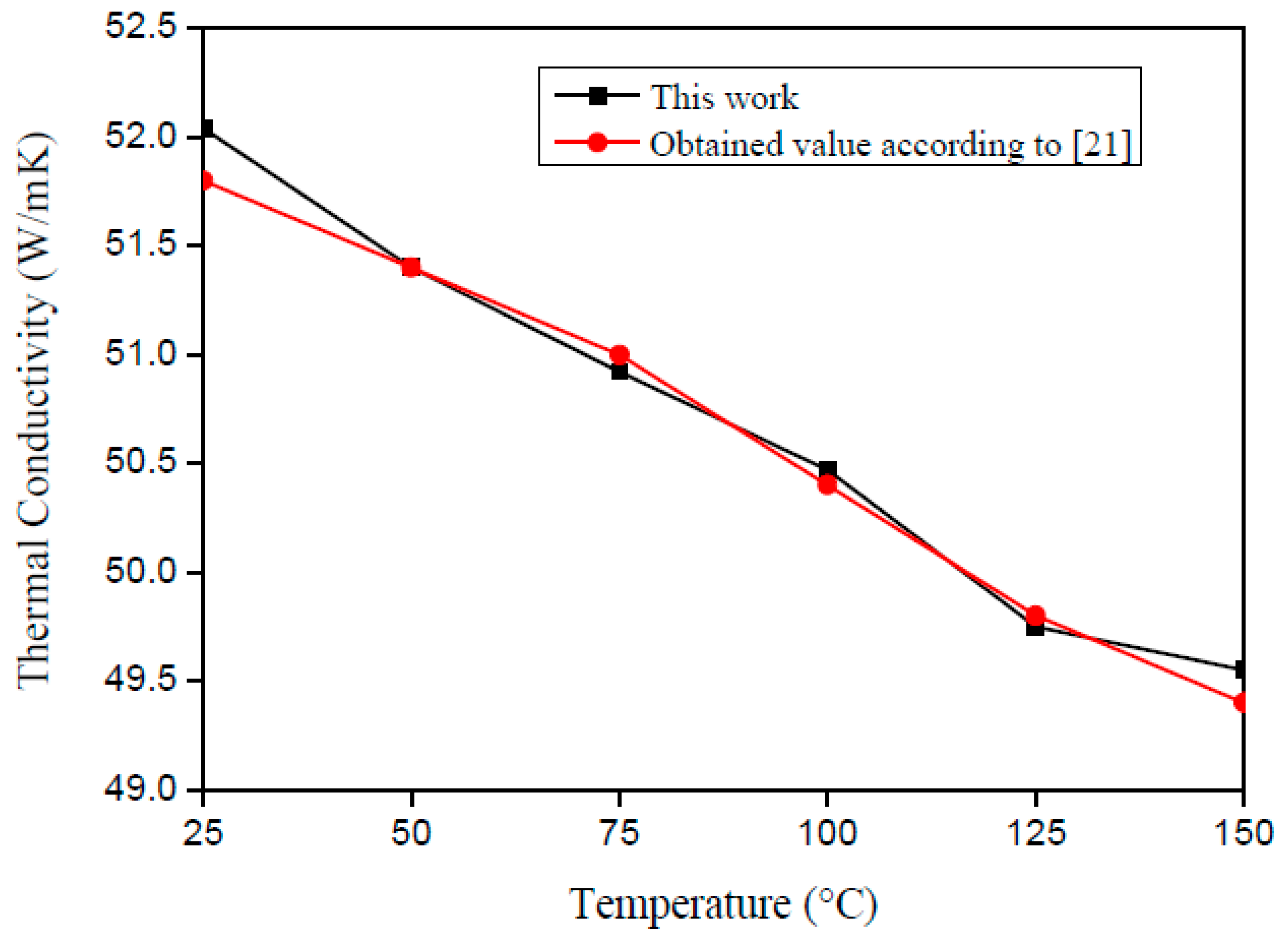
Figure 8 and Figure 9 present the literature and experimental result values. One can see the good agreement of the curves, which present a correlation factor of 0.98 for λ and 0.99 for ρcp. In accordance with Montgomery and Runger [22], the correlation factor indicates a quantitative measurement between two factors. Moreover, when the correlation factor presents value from +0.9 up to +1.0, it is possible to say that the correlation is direct and reliable.
From these results, Equations (7) and (8) can be written as follows for ρcp and λ, respectively:
These equations can be used in the range of 25 °C up to 150 °C.
3.2. AISI 304 Stainless Steel
Following the same procedure that was applied for the AISI 1045 steel sample, 15 experiments were performed for each initial condition (25 °C, 50 °C, 75 °C, 100 °C, 125 °C, and 150 °C) to estimate ρcp and λ simultaneously. Each experiment lasted 150 s following this condition: 0–20 s with a heat flux of 2672 Wm−2; 20–140 s with 668 Wm−2, and 140–150 s without a heat flux.
Figure 10 and Figure 11 present the sensitivity coefficients and the objective function, respectively, for each property. It can be seen that the behavior found was the same as the AISI 1045 steel, so it is possible to estimate the properties simultaneously. By analyzing the sensitivity coefficient of both materials, it is possible to affirm that the thermal conductivity estimation could be more precisely for AISI 304 stainless steel than 1045 steel. This is because there is more time for information, in other words, more points to analyze, and the difference between the values of the sensitivity coefficients for both properties are lower. This behavior is a consequence of the lower thermal conductivity of stainless steel when it is compared to 1045 steel.
Figure 12 shows the results for the analysis of the best experimental configuration. The maximum deviation found, around 0.05 °C, was lower than the uncertainty of the thermocouple, which confirms the reliability of the results and the good experimental configuration defined based on Figure 10 and Figure 11.
The imposed heat flux and the temperatures are presented in Figure 13. By analyzing this figure, one can see the good concordance between the temperatures. To validate this affirmation, the temperature residuals, where the maximum deviation was 0.05 °C, are presented in Figure 14. If this value was compared to the temperature difference, around 3 °C, one could see the good quality of the obtained results.
The results of ρcp and λ on the AISI 304 stainless steel sample for each initial temperature are presented in Table 2. Based on the lower standard deviation and the error found, the estimated values of ρcp and λ show a good conformity when compared to the literature values. This affirmation is based on the low standard deviation and error found. Similar to AISI 1045 steel, one may see that the results of ρcp are more precise due to its higher sensitivity.
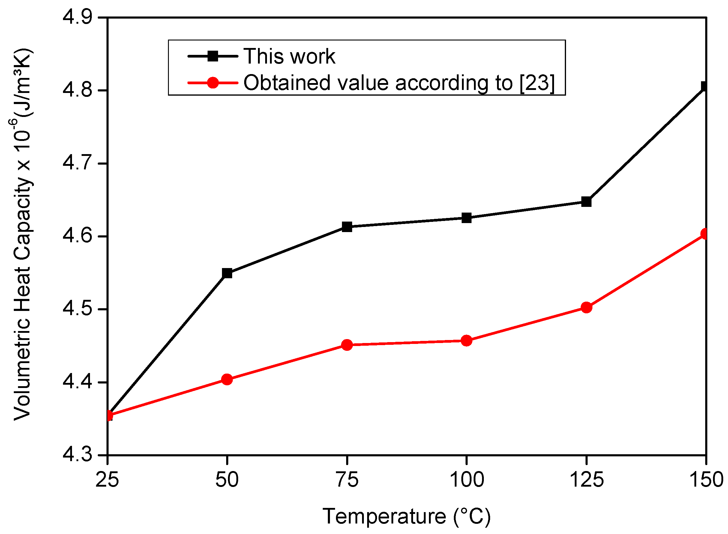
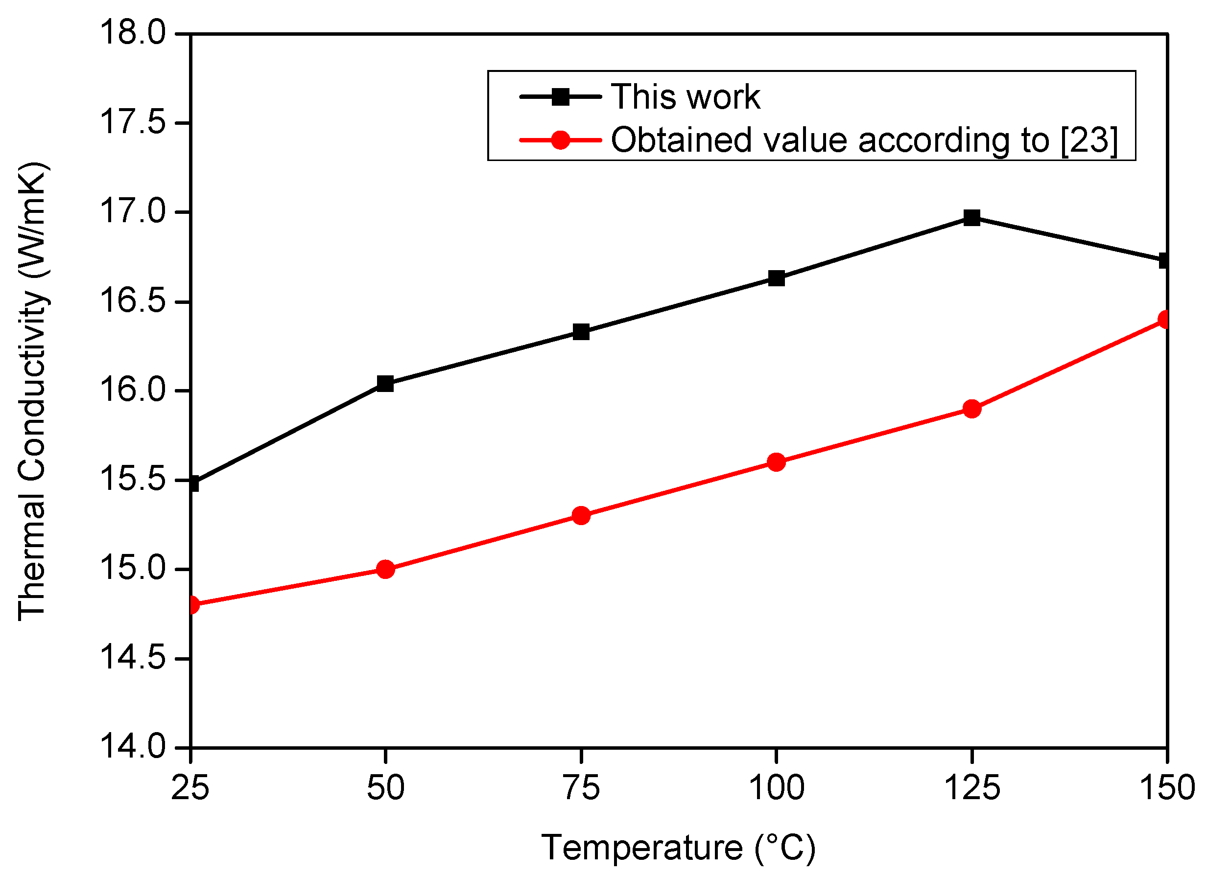
Figure 15 and Figure 16 present the literature and experimental result values. On analyzing Figure 15 and Figure 16, it is possible to verify the good agreement between the obtained results and those from the literature. To validate this affirmation, a correlation study was performed, and the correlation factor was 0.86 for λ and 0.95 for ρcp.
From these results, Equations (9) and (10) can be written as follows for ρcp and λ respectively:
These equations can be used in the range from 25 °C to 150 °C.
4. Uncertainty Analysis
The uncertainty propagation was considered to perform this analysis, as described in Carollo et al. [17] and Taylor [24], and it is important to assure the reliability of the estimated results.
Equations (11) and (12) show the uncertainty estimation based on the objective function (Equation (6)):
Individual uncertainty, which was divided by the mean value of the parameter, was used to calculate the partial uncertainty. Therefore, Table 3 presents the final uncertainty. One can see that these values are acceptable once they are around 5%.
5. Conclusions
This paper presents a different approach for the estimation of λ and ρcp in metallic materials simultaneously depending on temperature. The materials analyzed were the AISI 304 stainless steel and AISI 1045 steel. The good results found can be confirmed since the difference between the estimated values and literature is small, that is, lower than 7%, the standard deviation is the low, and the good uncertainty values are lower than 6%.
This work is validated to estimate λ and ρcp simultaneously in metals. However, this technique may be applied to reliably estimate λ and ρcp of metals that present thermal conductivity from 10 W/mK to 60 W/mK in a range of 25 °C up to 150 °C.
For future work, the use of a thermal model designed in three dimensions should be used to analyze the locations of temperature sensors in different positions to determine the areas that display better sensitivity to estimate λ and ρcp.
Author Contributions
L.F.d.S.C. developed the methodology, conceived and wrote the paper; A.L.F.d.L.e.S. was the co-advisor of this work; and S.M.M.d.L.e.S. is a specialist in heat transfer and was the advisor of this work.
Funding
The authors would like to thank CNPq, FAPEMIG, and CAPES for their financial support.
Conflicts of Interest
The authors declare no conflict of interest. The founding sponsors had no role in the design of the study; in the collection, analyses, or interpretation of data; in the writing of the manuscript, or in the decision to publish the results.
References
- Santos, M.R.; Lima e Silva, S.M.M.; Machado, A.R.; Silva, M.B.; Guimarães, G.; Carvalho, S.R. Analysis of Effects of Cutting Parameters on Cutting Edge Temperature Using Inverse Heat Conduction Technique. Math. Prob. Eng. 2014, 2014, 1–11. [Google Scholar] [CrossRef]
- Brito, R.F.; Carvalho, S.R.; Lima e Silva, S.M.M. Investigation of Thermal Aspects in a Cutting Tool Using Comsol and Inverse Problem. Appl. Therm. Eng. 2015, 86, 60–68. [Google Scholar] [CrossRef]
- Jannot, Y.; Degiovanni, A.; Payet, G. Thermal conductivity measurement of insulating materials with a three layers device. Int. J. Heat Mass Transf. 2009, 52, 1105–1111. [Google Scholar] [CrossRef]
- Xamán, J.; Lira, L.; Arce, J. Analysis of the temperature distribution in a guarded hot plate apparatus for measuring thermal conductivity. Appl. Therm. Eng. 2009, 29, 617–623. [Google Scholar] [CrossRef]
- Thomas, M.; Boyard, N.; Lefèvre, N.; Jarny, Y.; Delaunay, D. An experimental device for the simultaneous estimation of the thermal conductivity 3-D tensor and the specific heat of orthotropic composite materials. Int. J. Heat Mass Transf. 2010, 53, 5487–5498. [Google Scholar] [CrossRef]
- Aksöz, S.; Ocak, Y.; Marasli, N.; Cadirli, E.; Kaya, H.; Böyük, U. Dependency of the Thermal and Electrical Conductivity on the Temperature and Composition of Cu in the Al based Al–Cu Alloys. Exp. Therm. Fluid Sci. 2010, 34, 1507–1516. [Google Scholar] [CrossRef]
- Karimi, G.; Li, X.; Teerstra, P. Measurement of Through-plane Effective Thermal Conductivity and Contact Resistance in PEM Fuel Cell Diffusion. Media Electrochim. Acta 2010, 55, 1619–1625. [Google Scholar] [CrossRef]
- Sadeghi, E.; Djilali, N.; Bahrami, M. A Novel Approach to Determine the In-plane Thermal Conductivity of Gas Diffusion Layers in Proton Exchange Membrane Fuel Cells. J. Power Sources 2011, 196, 3565–3571. [Google Scholar] [CrossRef]
- Zamel, N.; Becker, J.; Wiegmann, A. Estimating the Thermal Conductivity and Diffusion Coefficient of the Microporous Layer of Polymer Electrolyte Membrane Fuel Cells. J. Power Sources 2012, 207, 70–80. [Google Scholar] [CrossRef]
- Öztürk, E.; Aksöz, S.; Keslioglu, K.; Marasli, N. The Measurement of Thermal Conductivity variation with Temperature for Sn-20 wt.% in based Lead-free Ternary Solders. Thermochim. Acta 2013, 554, 63–70. [Google Scholar] [CrossRef]
- Zgraja, J.; Cieslak, A. Induction heating in estimation of thermal properties of conductive materials. Int. J. Comput. Math. Electr. Electron. Eng. 2017, 36, 458–468. [Google Scholar] [CrossRef]
- Somasundharam, S.; Reddy, K.S. Simultaneously estimation of thermal properties of orthotropic material with non-intrusive measurement. Int. J. Heat Mass Transf. 2018, 126, 1162–1177. [Google Scholar] [CrossRef]
- García, E.; Amaya, I.; Correa, R. Estimation of thermal properties of a solid sample during a microwave heating process. Appl. Therm. Eng. 2018, 129, 587–595. [Google Scholar] [CrossRef]
- Lembcke, L.G.M.; Roubinet, D.; Gidel, F.; Irving, J.; Pehme, P.; Parker, B.L. Analytical analysis of borehole experiments for the estimation of subsurface thermal properties. Adv. Water Resour. 2016 91, 88–103.
- Ren, Y.; Qi, H.; He, M.; Ruan, S.; Ruan, L.; Tan, H. Application of an improved firework algorithm for simultaneous estimation of temperature-dependent thermal and optical properties of molten salt. Int. Commun. Heat Mass Transf. 2016, 77, 33–42. [Google Scholar] [CrossRef]
- Udayraj; Talukdar, P.; Das, A.; Alagirusamy, R. Simultaneous estimation of thermal conductivity and specific heat of thermal protective fabrics using experimental data of high heat flux exposure. Appl. Therm. Eng. 2016, 107, 785–796. [Google Scholar] [CrossRef]
- Carollo, L.F.S.; Lima e Silva, A.L.F.; Lima e Silva, S.M.M. Applying Different Heat Flux Intensities to Simultaneously Estimate the Thermal Properties of Metallic Materials. Meas. Sci. Technol. 2012, 23, 1–10. [Google Scholar] [CrossRef]
- Özisik, M.N. Heat Conduction; John Wiley & Sons: Etobicoke, ON, Canada, 1993; p. 692. [Google Scholar]
- Tillmann, A.R.; Borges, V.L.; Guimarães, G.; Lima e Silva, A.L.F.; Lima e Silva, S.M.M. Identification of Temperature-Dependent Thermal Properties of Solid Materials. J. Braz. Soc. Mech. Sci. Eng. 2008, 30, 269–278. [Google Scholar] [CrossRef]
- Vanderplaats, G.N. Numerical Optimization Techniques for Engineering Design; McGraw: New York, NY, USA, 2005; p. 465. [Google Scholar]
- Grzesik, W.; Nieslony, P.; Bartoszuk, M. Modelling of the Cutting Process Analytical and Simulation Methods. Adv. Manuf. Sci. Technol. 2009, 33, 6–29. [Google Scholar]
- Montgomery, D.C.; Runger, G.C. Applied Statistic and Probability for Engineers; John Wiley & Sons: New York, NY, USA, 2013; p. 811. [Google Scholar]
- Abas, R.A.; Hayashi, M.; Seetharaman, S. Thermal Diffusivity Measurements of Some Industrially Important Alloys by a Laser Flash Method. Int. J. Mater. Res. 2009, 98, 1–6. [Google Scholar] [CrossRef]
- Taylor, J.R. An Introduction to Error Analysis: The Study of Uncertainties in Physical Measurements; University Science Books: Sausalito, CA, USA, 1997; p. 488. [Google Scholar]
Figure 1.
A one-dimensional (1D) representation of the model. (a) thermal model; (b) three-dimensional view of the thermal model.
Figure 1.
A one-dimensional (1D) representation of the model. (a) thermal model; (b) three-dimensional view of the thermal model.

Figure 2.
Experimental apparatus sketch used to estimate ρcp and λ.

Figure 3.
AISI 1045 steel with its corresponding sensitivity coefficients.

Figure 4.
Values of F (Equation (6)) for AISI 1045 steel.

Figure 5.
Results of the ideal condition and design for the experiment on AISI 1045.

Figure 6.
Experimental heat flow () for AISI 1045. Comparison of temperatures obtained numerically (T) and experimentally (Y).
Figure 6.
Experimental heat flow () for AISI 1045. Comparison of temperatures obtained numerically (T) and experimentally (Y).

Figure 7.
Residuals of temperatures of AISI 1045.

Figure 8.
Comparison between the literature values with the estimated results of ρcp on the AISI 1045 steel plate.
Figure 8.
Comparison between the literature values with the estimated results of ρcp on the AISI 1045 steel plate.

Figure 9.
Comparison between the literature values with the estimated results of λ on the AISI 1045 steel sample.
Figure 9.
Comparison between the literature values with the estimated results of λ on the AISI 1045 steel sample.

Figure 10.
Sensitivity coefficient of the AISI 304 stainless steel sample.

Figure 11.
Values of the objective function for the AISI 304 sample.

Figure 12.
Results of the ideal condition and design for the experiment with AISI 304.

Figure 13.
Experimental heat flow () for AISI 304. Comparison of temperatures obtained numerically (T) and experimentally (Y).
Figure 13.
Experimental heat flow () for AISI 304. Comparison of temperatures obtained numerically (T) and experimentally (Y).

Figure 14.
Residuals of temperature of AISI 304.

Figure 15.
Comparison between the literature values with the estimated results of ρcp on the AISI 304 stainless steel sample.
Figure 15.
Comparison between the literature values with the estimated results of ρcp on the AISI 304 stainless steel sample.

Figure 16.
Comparison between the literature values with the estimated results of λ on the AISI 304 stainless steel sample.
Figure 16.
Comparison between the literature values with the estimated results of λ on the AISI 304 stainless steel sample.


Table 1.
Average results, standard deviation, and error of ρcp and λ for AISI 1045.
| Average T0 (°C) | Thermal Properties | Mean | Obtained value from Grzesik et al. [21] | Standard Deviation | Error (%) |
|---|---|---|---|---|---|
| 25.4 | ρcp × 10−6 (J/m³K) | 3.48 | 3.43 | ±0.02 | 1.44 |
| λ (W/mK) | 52.04 | 51.80 | ±0.49 | 0.46 | |
| 50.1 | ρcp ×10−6 (J/m³K) | 3.54 | 3.50 | ±0.05 | 1.18 |
| λ (W/mK) | 51.39 | 51.4 | ±0.25 | 0.02 | |
| 75.4 | ρcp × 10−6 (J/m³K) | 3.59 | 3.54 | ±0.04 | 1.36 |
| λ (W/mK) | 50.92 | 51.00 | ±0.37 | 0.16 | |
| 100.4 | ρcp × 10−6 (J/m³K) | 3.61 | 3.66 | ±0.03 | 0.99 |
| λ (W/mK) | 50.47 | 50.40 | ±0.28 | 0.14 | |
| 125.3 | ρcp × 10−6 (J/m³K) | 3.66 | 3.61 | ±0.05 | 1.42 |
| λ (W/mK) | 49.75 | 49.80 | ±0.38 | 0.10 | |
| 150.2 | ρcp × 10−6 (J/m³K) | 3.74 | 3.77 | ±0.02 | 0.86 |
| λ (W/mK) | 49.55 | 49.40 | ±0.36 | 0.30 |
Table 2.
Results obtained for the AISI 304 stainless steel sample.
| Average T0 (°C) | Thermal Properties | Mean | Obtained value from Abas et al. [23] | Standard Deviation | Error (%) |
|---|---|---|---|---|---|
| 24.8 | ρcp × 10−6 (J/m³K) | 4.35 | 4.35 | ±0.12 | 0.03 |
| λ (W/mK) | 15.49 | 14.8 | ±0.39 | 4.64 | |
| 49.7 | ρcp × 10−6 (J/m³K) | 4.55 | 4.40 | ±0.09 | 3.31 |
| λ (W/mK) | 16.04 | 15.0 | ±0.58 | 6.95 | |
| 74.9 | ρcp × 10−6 (J/m³K) | 4.61 | 4.45 | ±0.06 | 3.64 |
| λ (W/mK) | 16.33 | 15.3 | ±0.47 | 6.76 | |
| 99.2 | ρcp × 10−6 (J/m³K) | 4.63 | 4.46 | ±0.07 | 3.77 |
| λ (W/mK) | 16.63 | 15.6 | ±0.53 | 6.62 | |
| 124.9 | ρcp × 10−6 (J/m³K) | 4.65 | 4.50 | ±0.06 | 3.22 |
| λ (W/mK) | 16.97 | 15.9 | ±0.57 | 6.74 | |
| 149.5 | ρcp × 10−6 (J/m³K) | 4.80 | 4.60 | ±0.09 | 4.38 |
| λ (W/mK) | 16.73 | 16.4 | ±0.67 | 2.01 |
Table 3.
Uncertainty values for each analyzed material.
| Material | Uncertainty (%) |
|---|---|
| AISI 1045 steel | 5.45 |
| AISI 304 stainless steel | 4.79 |
© 2019 by the authors. Licensee MDPI, Basel, Switzerland. This article is an open access article distributed under the terms and conditions of the Creative Commons Attribution (CC BY) license (http://creativecommons.org/licenses/by/4.0/).
Share and Cite
MDPI and ACS Style
Carollo, L.F.d.S.; Lima e Silva, A.L.F.d.; Lima e Silva, S.M.M.d. A Different Approach to Estimate Temperature-Dependent Thermal Properties of Metallic Materials. Materials 2019, 12, 2579. https://doi.org/10.3390/ma12162579
AMA Style
Carollo LFdS, Lima e Silva ALFd, Lima e Silva SMMd. A Different Approach to Estimate Temperature-Dependent Thermal Properties of Metallic Materials. Materials. 2019; 12(16):2579. https://doi.org/10.3390/ma12162579
Chicago/Turabian StyleCarollo, Luís Felipe dos Santos, Ana Lúcia Fernandes de Lima e Silva, and Sandro Metrevelle Marcondes de Lima e Silva. 2019. "A Different Approach to Estimate Temperature-Dependent Thermal Properties of Metallic Materials" Materials 12, no. 16: 2579. https://doi.org/10.3390/ma12162579
Note that from the first issue of 2016, this journal uses article numbers instead of page numbers. See further details here.