Prediction and Analysis of the Residual Capacity of Concrete-Filled Steel Tube Stub Columns under Axial Compression Subjected to Combined Freeze–Thaw Cycles and Acid Rain Corrosion


Abstract
:1. Introduction
2. Development and Validation of the Finite Element Model
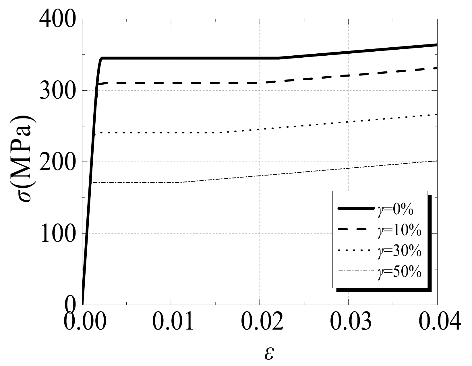
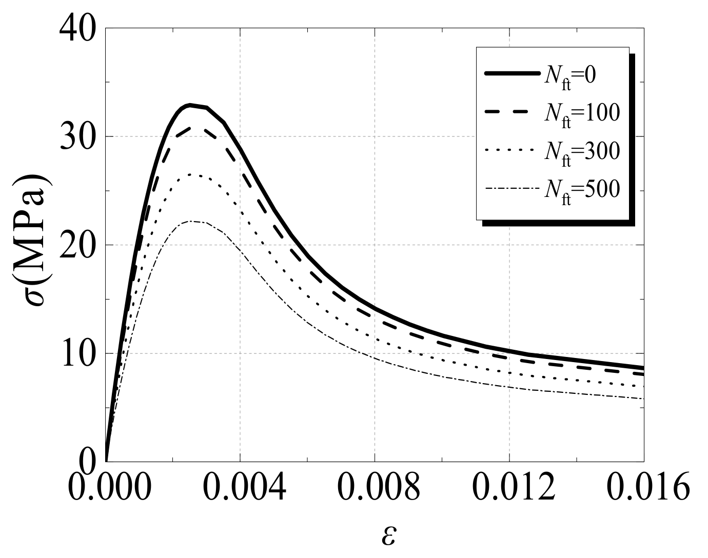
2.1. Stress–Strain Relationships of Materials
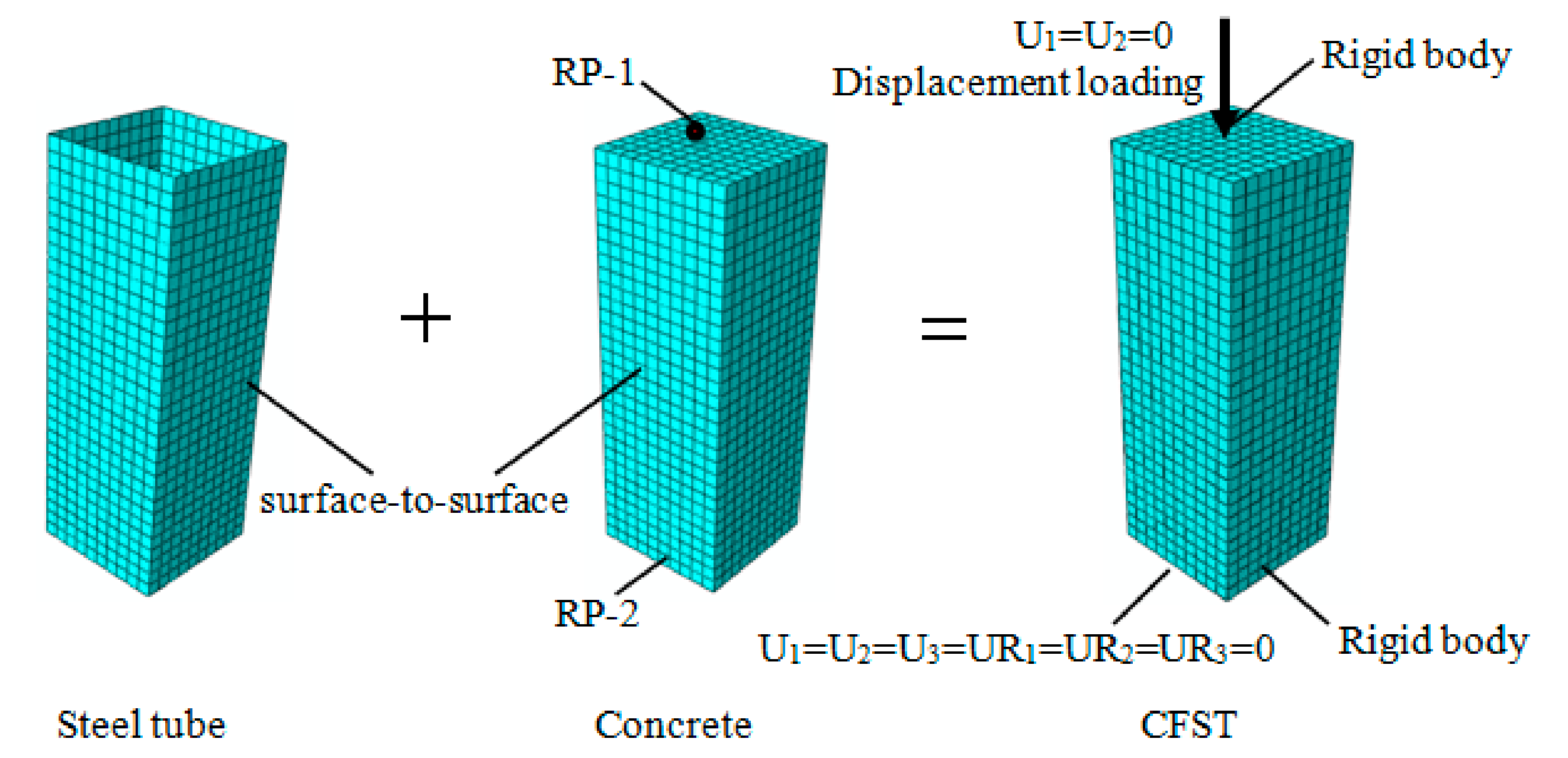
2.2. Numerical Modeling
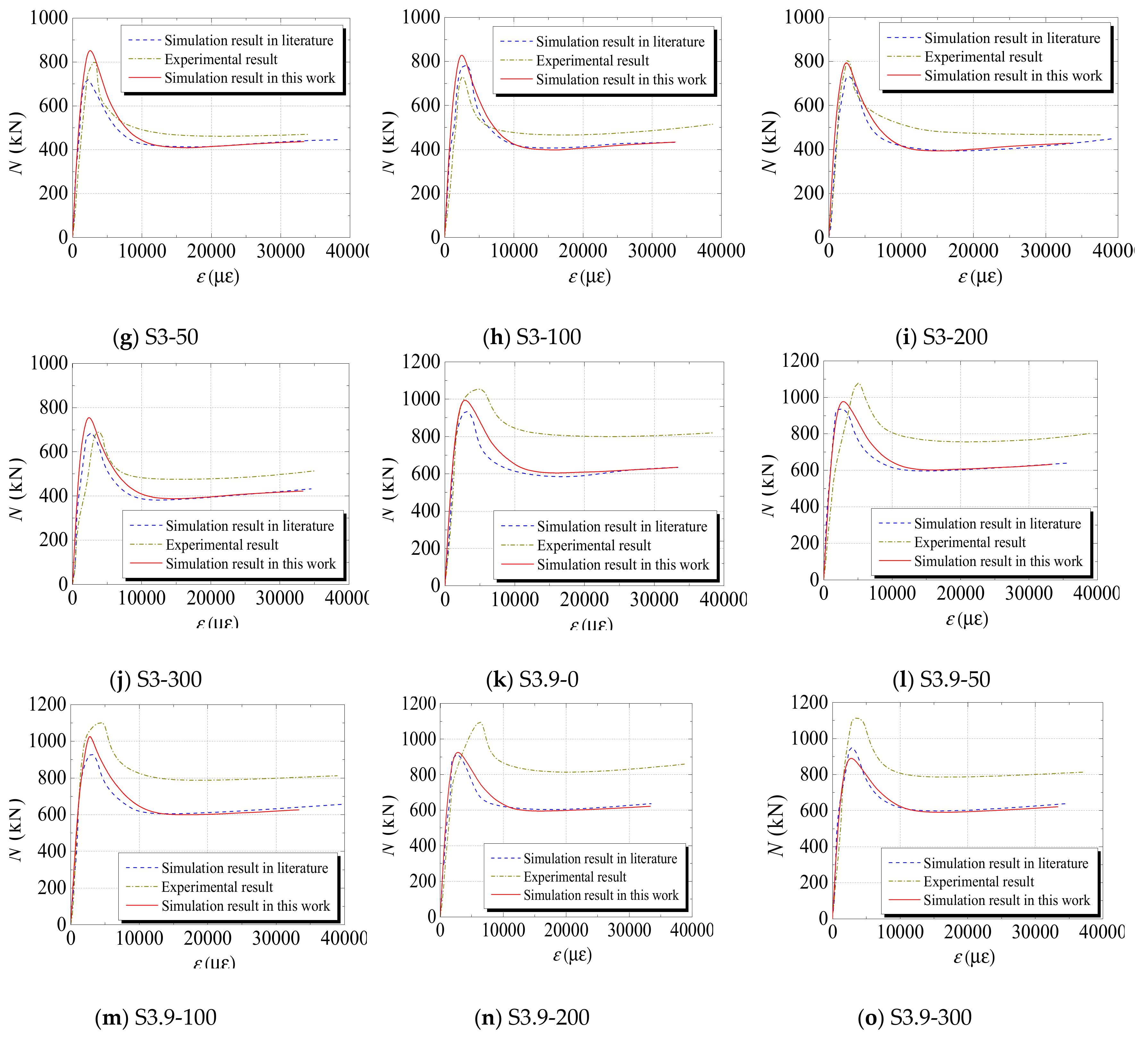
2.3. Verification of the FE Model
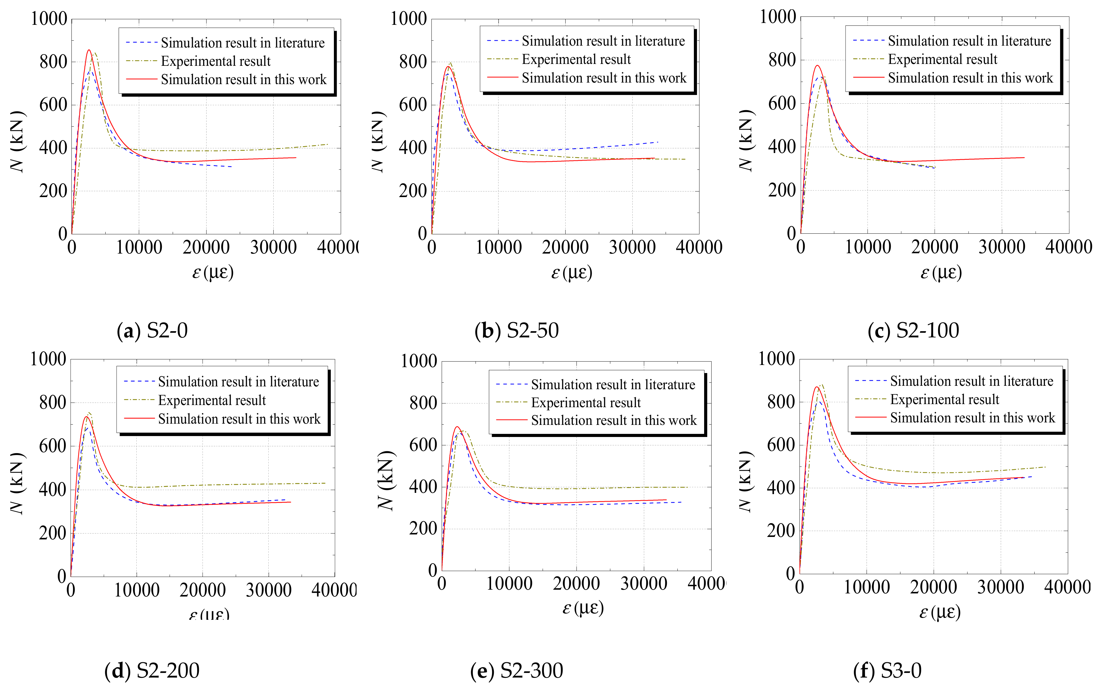
2.3.1. Experimental Validation of the Freeze–Thaw Cycle Case
- (1)
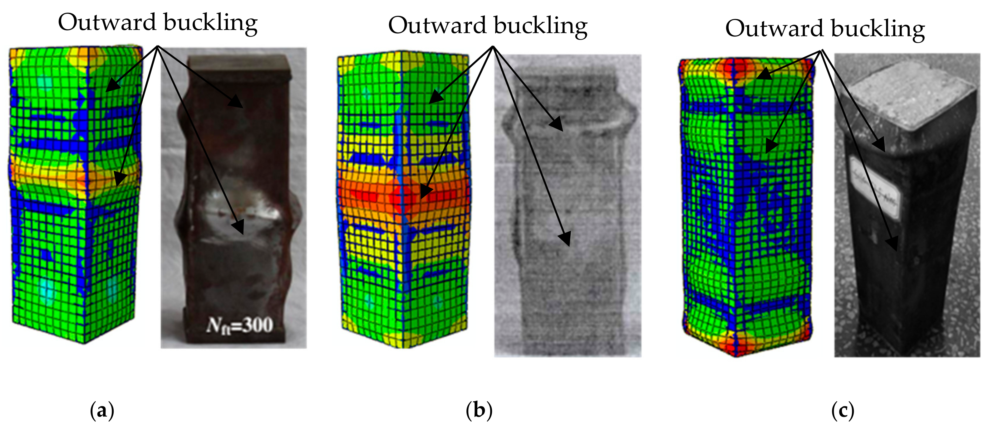
- Failure Mode
- (2)
- Bearing Capacity
- (3)
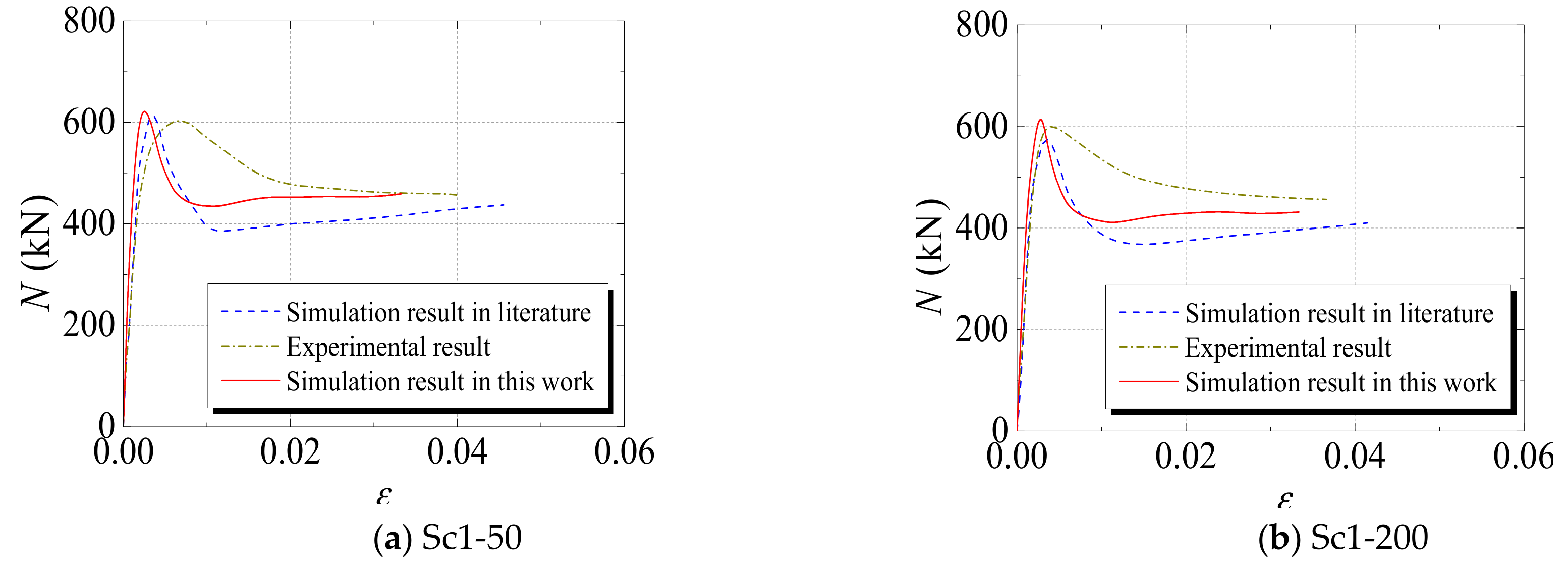
- Axial Load–Displacement (or Strain) Curve
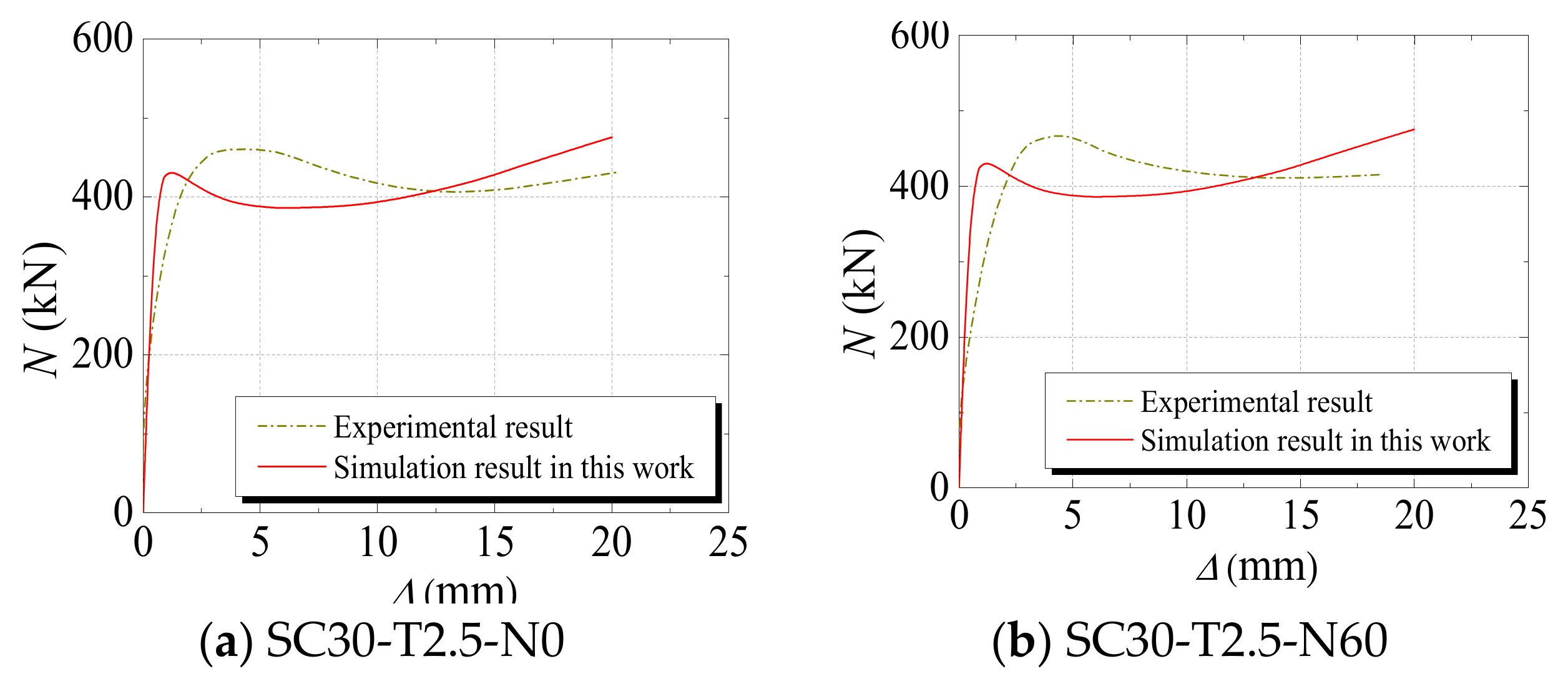
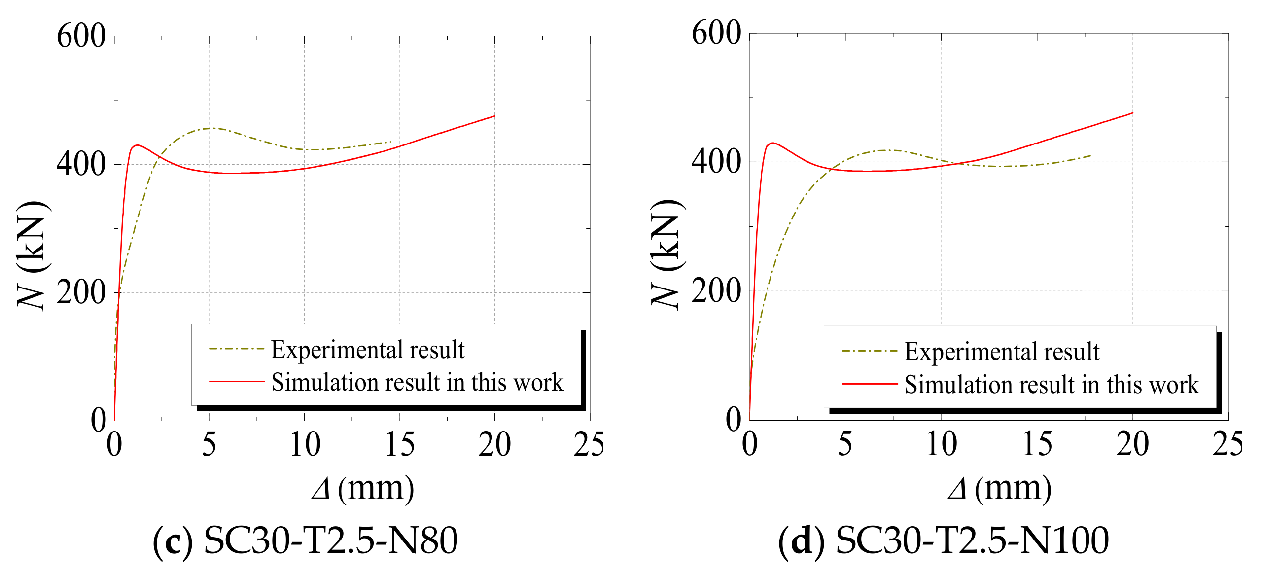
2.3.2. Experimental Validation of the Acid Rain Corrosion Case
2.3.3. Analysis of Validation Results
3. Whole-Process Analysis of the Load–Displacement Relationship
3.1. Numerical Modeling for Axial Compression
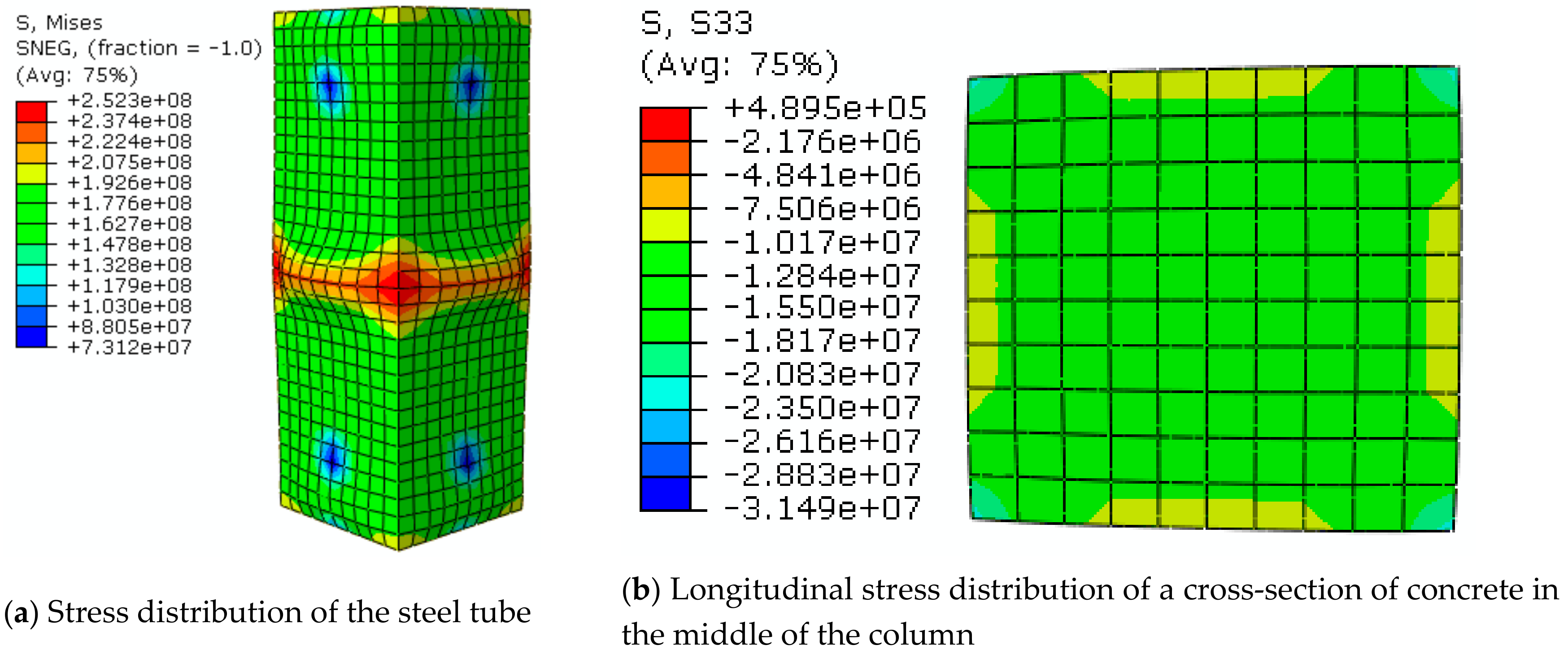
3.2. Failure Mode
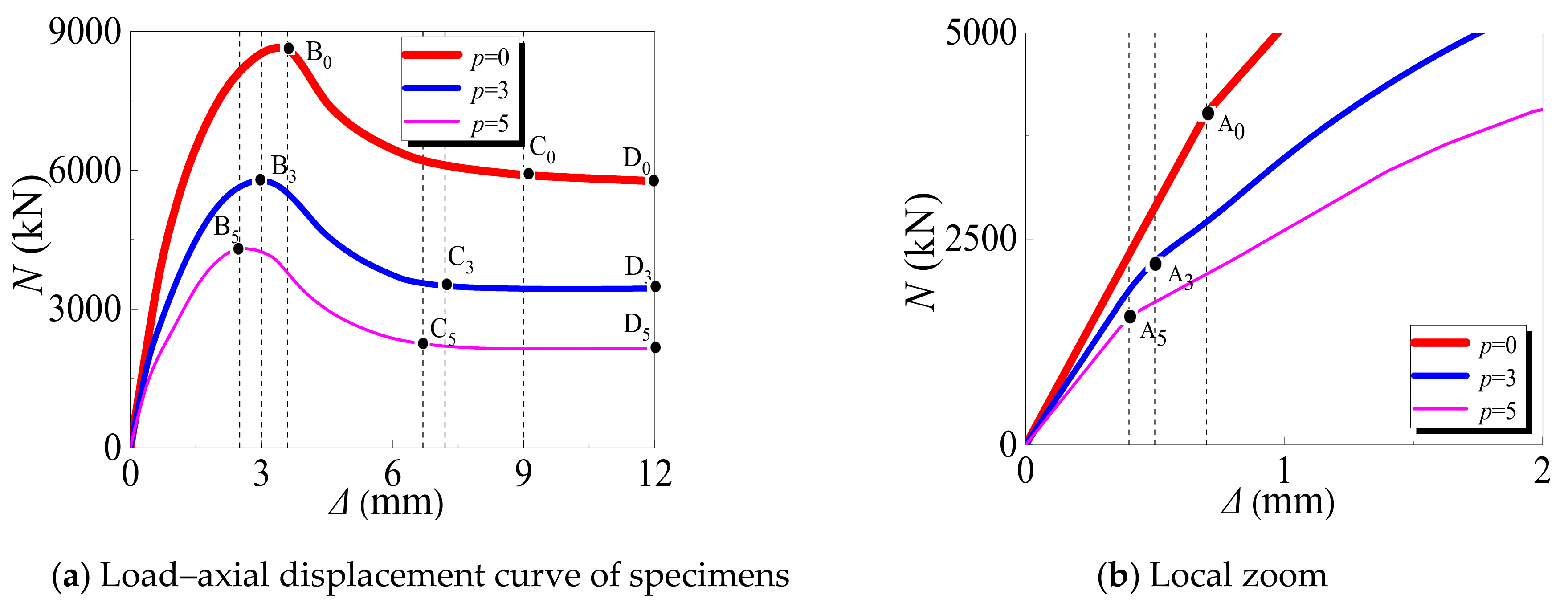
3.3. Load–Axial Displacement Relationship Curve
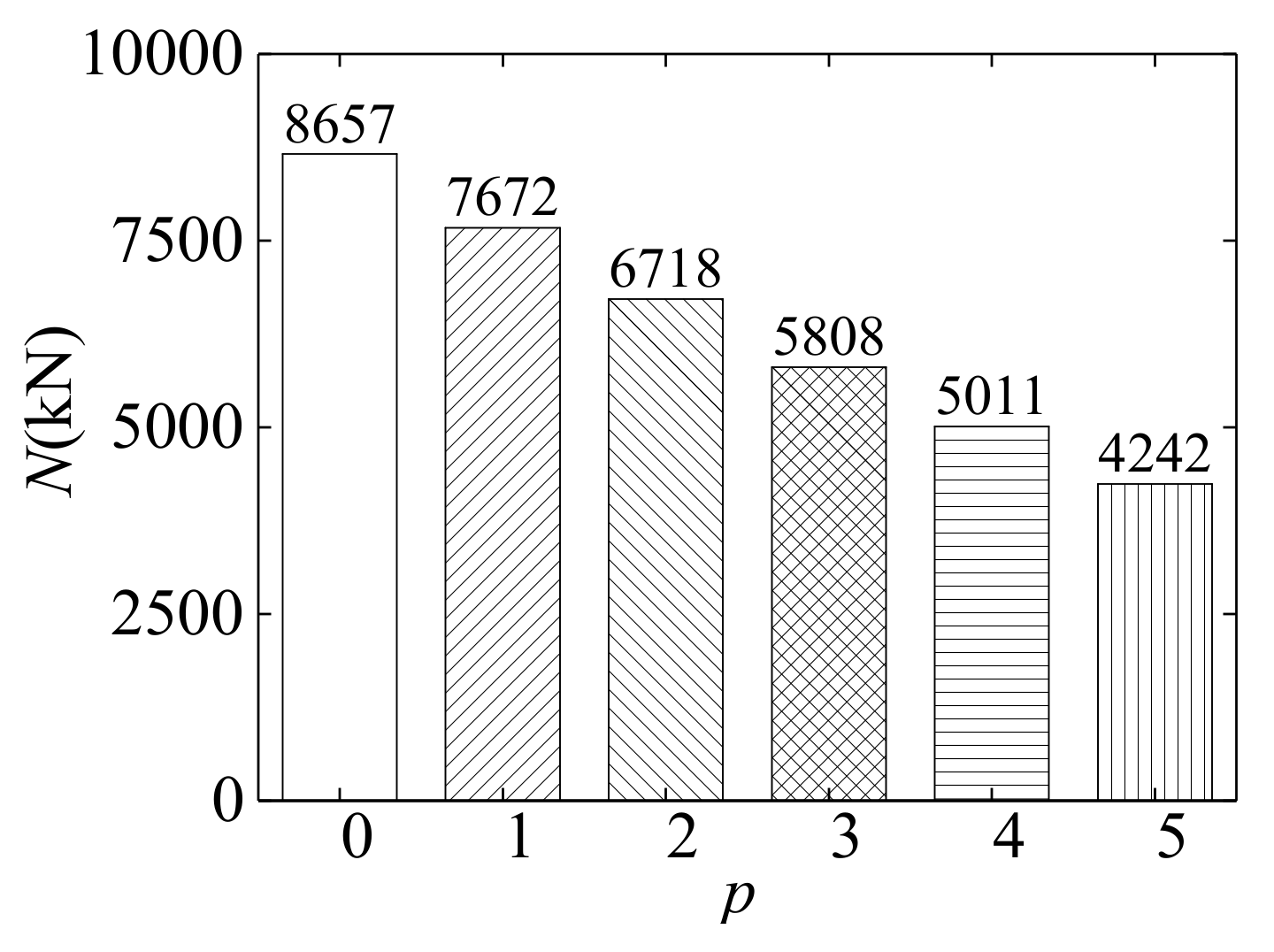
3.4. Bearing Capacity
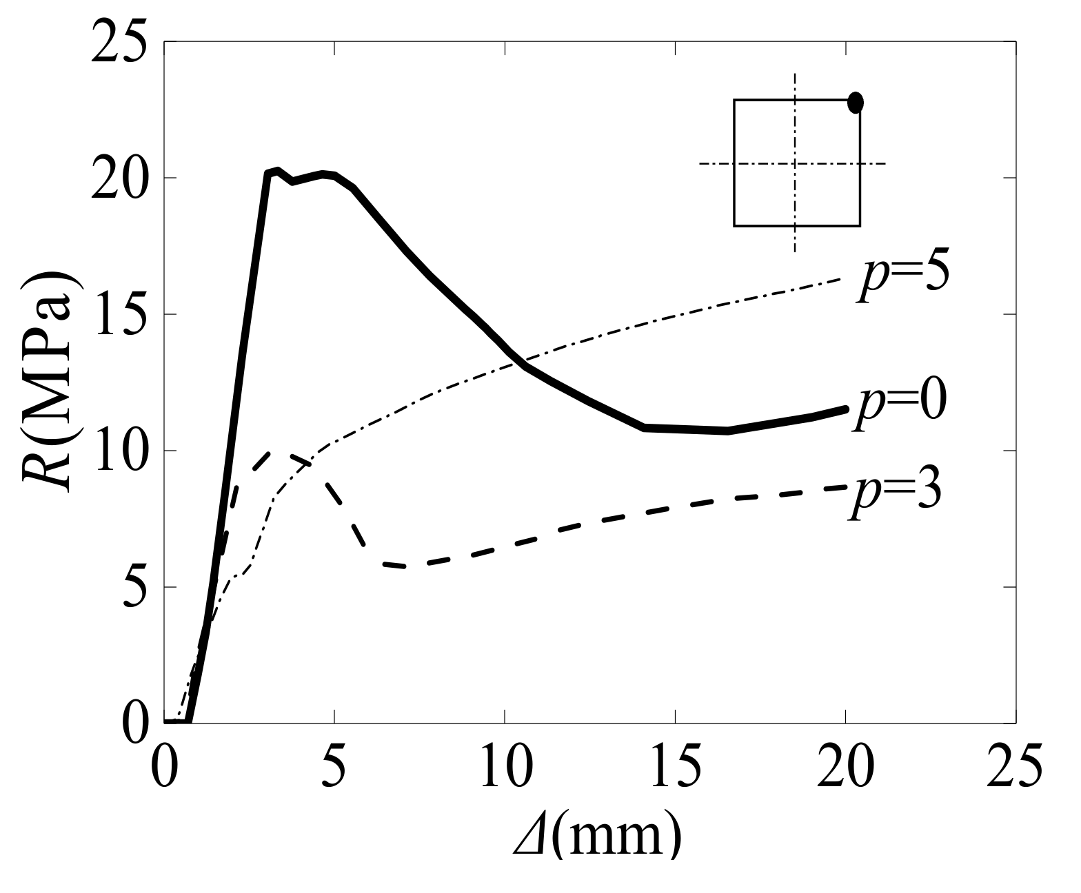
3.5. Interaction between the Steel Tube and Core Concrete
4. Parameter Analysis and Design Method of Bearing Capacity
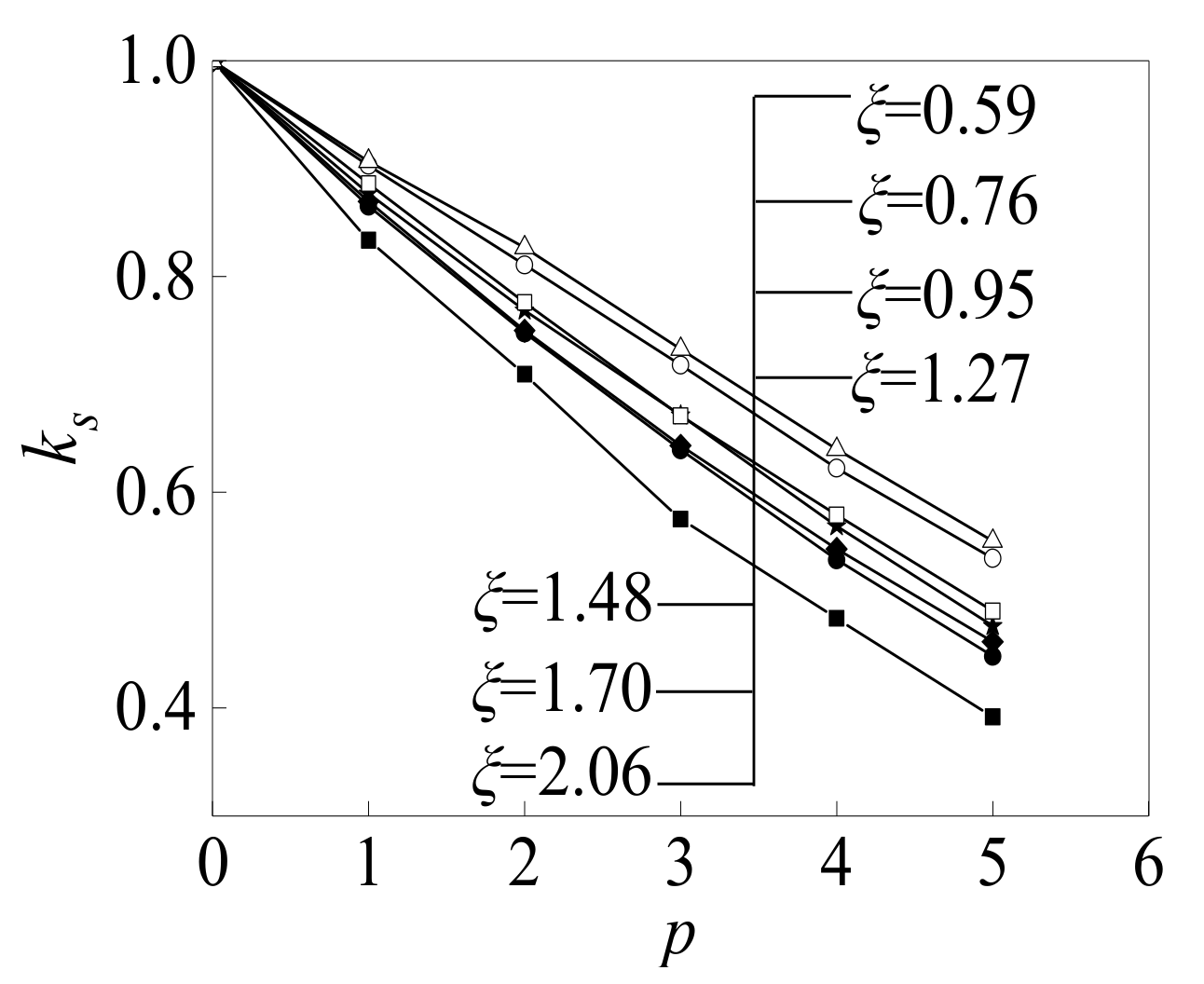
4.1. Parameter Analysis
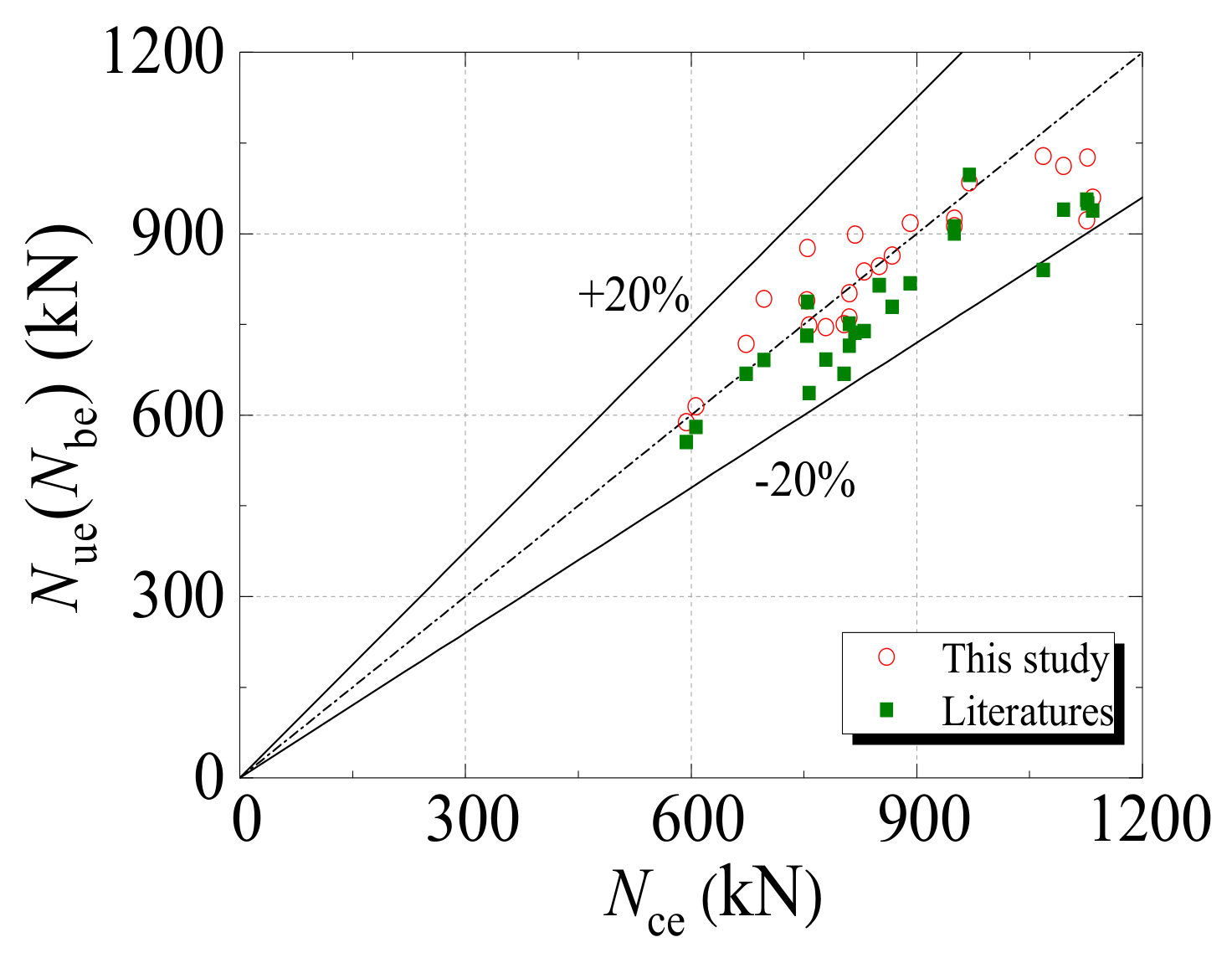
4.2. Design Formulae
5. Conclusions
- (1)
- The failure mode of SCFST stub columns subjected to freeze–thaw cycles and acid rain corrosion is similar to that of columns without any action after they are axially loaded. Buckling occurs at both ends and in the central height of the columns. With the increase in the combined times, the local buckling amplitude of the steel tube increases.
- (2)
- The load–displacement curves of SCFST stub columns under axial compression are basically the same after the columns are subjected to the combined action of freeze–thaw cycles and acid rain corrosion. All the curves include the elastic stage, elastic-plastic stage, descending stage, and stable stage. Under the same conditions, as the combination times increase, the times at which the specimens arrive at each stage are earlier. Regardless of whether the specimens undergo a combination of freeze–thaw cycles and acid rain corrosion, they all have stable bearing capacities in the later stage, and the failure type is a plastic failure.
- (3)
- The parameters that influence the ultimate bearing capacity of the specimens after freeze–thaw cycles and acid rain corrosion include the restraint effect coefficient (ζe) and combination times (p), which cannot be neglected. Generally, the larger the restraint effect coefficient or the combination times, the smaller the influence factor (Ks) of the residual bearing capacity.
- (4)
- From the result of parameter analysis, design formulae are proposed for predicting the bearing capacity of the SCFST column that is under axial compression and subjected to the combined action of freeze–thaw cycles and acid rain corrosion.
Author Contributions
Funding
Conflicts of Interest
References
- Hua, Y.X.; Han, L.H.; Wang, Q.L.; Hou, C. Behaviour of square CFST beam-Columns under combined sustained load and corrosion: Experiments. Thin-Walled Struct. 2019, 136, 353–366. [Google Scholar] [CrossRef]
- Lyu, X.; Xu, Y.; Xu, Q.; Yu, Y. Axial compression performance of square thin walled concrete-Filled steel tube stub columns with reinforcement stiffener under constant high-Temperature. Materials 2019, 12, 1098. [Google Scholar] [CrossRef] [PubMed]
- Yang, Z.; Xu, C. Research on compression behavior of square thin-Walled CFST columns with steel-Bar stiffeners. Appl. Sci. 2018, 8, 1602. [Google Scholar] [CrossRef]
- Wu, H.; Cao, W.; Qiao, Q.; Dong, H. Uniaxial compressive constitutive relationship of concrete confined by special-shaped steel tube coupled with multiple cavities. Materials 2016, 9, 86. [Google Scholar] [CrossRef] [PubMed]
- Qiao, Q.; Zhang, W.; Qian, Z.; Cao, W.; Liu, W. Experimental study on mechanical behavior of shear connectors of square concrete filled steel tube. Appl. Sci. 2017, 7, 818. [Google Scholar] [CrossRef]
- Liu, W.; Cao, W.; Zhang, J.; Wang, R.; Ren, L. Mechanical behavior of recycled aggregate concrete-Filled steel tubular columns before and after fire. Materials 2017, 10, 274. [Google Scholar] [CrossRef]
- Li, R.; Yu, Y.; Samali, B.; Li, C. Parametric analysis on the circular CFST column and RBS steel beam joints. Materials 2019, 12, 1535. [Google Scholar] [CrossRef]
- Technical Code for Concrete Filled Steel Tubular Structures; GB50936-2014; Ministry of Housing and Urban-Rural Development of the People’s Republic of China (MOHURD): Beijing, China, 2014.
- Technical Specification for Structures with Concrete-Filled Rectangular Steel Tube Members; CECS159-2004; China Association for Engineering Construction Standardization: Beijing, China, 2004.
- Steel, Concrete and Composite Bridges Part 5: Code of Practice for the Design of Composite Bridges; BS 5400-5:2005; British Standards Institution: London, UK, 2005.
- Eurocode 4: Design of Composite Steel and Concrete Structures, Part 1.1. General Rules and Rules for Buildings. EN 1994-1-1; British Standards Institution: London, UK, 2004.
- ACI 318-05. Building Code Requirements for Structural Concrete and Commentary; American Concrete Institute: Farmington Hills, MI, USA, 2005. [Google Scholar]
- AIJ. Recommendations for Design and Construction of Concrete Filled Steel Tubular Structures; Architectural Institute of Japan: Tokyo, Japan, 2008. [Google Scholar]
- Du, Y.; Chen, Z.; Zhang, C.; Cao, X. Research on axial bearing capacity of rectangular concrete-Filled steel tubular columns based on artificial neural networks. Front. Comput. Sci. 2017, 11, 863–873. [Google Scholar] [CrossRef]
- Patel, V.I.; Hassanein, M.F.; Thai, H.T.; Al Abadi, H.; Elchalakani, M.; Bai, Y. Ultra-High strength circular short CFST columns: Axisymmetric analysis, behaviour and design. Eng. Struct. 2019, 179, 268–283. [Google Scholar] [CrossRef]
- Shams, M.; Saadeghvaziri, M.A. Nonlinear response of concrete-Filled steel tubular columns under axial loading. ACI Struct. J. 1999, 96, 1009–1017. [Google Scholar]
- Montuori, R.; Piluso, V. Analysis and modelling of CFT members: Moment curvature analysis. Thin-Walled Struct. 2015, 86, 157–166. [Google Scholar] [CrossRef]
- Susantha, K.A.S.; Ge, H.; Usami, T. Cyclic analysis and capacity prediction of concrete-Filled steel box columns. Earthq. Eng. Struct. Dyn. 2002, 31, 195–216. [Google Scholar] [CrossRef]
- Wang, X.T.; Xie, C.D.; Lin, L.H.; Li, J. Seismic behavior of self-Centering concrete-Filled square steel tubular (CFST) column base. J. Constr. Steel Res. 2019, 156, 75–85. [Google Scholar] [CrossRef]
- Wang, J.; Sun, Q.; Li, J. Experimental study on seismic behavior of high-Strength circular concrete-Filled thin-Walled steel tubular columns. Eng. Struct. 2019, 182, 403–415. [Google Scholar] [CrossRef]
- Zhou, K.; Han, L.H. Modelling the behaviour of concrete-Encased concrete-Filled steel tube (CFST) columns subjected to full-Range fire. Eng. Struct. 2019, 183, 265–280. [Google Scholar] [CrossRef]
- Yang, H.; Liu, F.; Gardner, L. Post-Fire behaviour of slender reinforced concrete columns confined by circular steel tubes. Thin-Walled Struct. 2015, 87, 12–29. [Google Scholar] [CrossRef]
- Yuan, F.; Chen, M.; Huang, H.; Xie, L.; Wang, C. Circular concrete filled steel tubular (CFST) columns under cyclic load and acid rain attack: Test simulation. Thin-Walled Struct. 2018, 122, 90–101. [Google Scholar] [CrossRef]
- Yang, Y.F.; Cao, K.; Wang, T.Z. Experimental behavior of CFST stub columns after being exposed to freezing and thawing. Cold Reg. Sci. Technol. 2013, 89, 7–21. [Google Scholar] [CrossRef]
- Wei, H.; Wu, Z.; Guo, X.; Yi, F. Experimental study on partially deteriorated strength concrete columns confined with CFRP. Eng. Struct. 2009, 31, 2495–2505. [Google Scholar] [CrossRef]
- Qin, Z.; Lai, Y.; Tian, Y.; Yu, F. Frost-Heaving mechanical model for concrete face slabs of earthen dams in cold regions. Cold Reg. Sci. Technol. 2019, 161, 91–98. [Google Scholar] [CrossRef]
- Zhang, G.; Yu, H.; Li, H.; Yang, Y. Experimental study of deformation of early age concrete suffering from frost damage. Constr. Build. Mater. 2019, 215, 410–421. [Google Scholar] [CrossRef]
- Zhang, X.; Jiang, H.; Zhang, Q.; Zhang, X. Chemical characteristics of rainwater in northeast China, a case study of Dalian. Atmos. Res. 2012, 116, 151–160. [Google Scholar] [CrossRef]
- Liu, M.; Song, Y.; Zhou, T.; Xu, Z.; Yan, C.; Zheng, M.; Wu, Z.; Hu, M.; Wu, Y.; Zhu, T. Fine particle pH during severe haze episodes in northern China. Geophys. Res. Lett. 2017, 44, 5213–5221. [Google Scholar] [CrossRef]
- Cheng, M.; Lin, B.; Huang, H. Research on the bearing capacity of corroded square concrete filled steel tubular short column. Steel Constr. 2017, 32, 110–116. [Google Scholar]
- Tao, Z.; Wang, Z.B.; Yu, Q. Finite element modelling of concrete-filled steel stub columns under axial compression. J. Constr. Steel Res. 2013, 89, 121–131. [Google Scholar] [CrossRef]
- Tian, J. Behavior of Eccentricity Loaded Circular Stainless Steel-Carbon Steel Composite Tube Confined Concrete Columns. Ph.D. Thesis, Harbin Institute of Technology, Harbin, China, 2017. [Google Scholar]
- Han, L.H.; Yao, G.H.; Tao, Z. Performance of concrete-Filled thin-Walled steel tubes under pure torsion. Thin-Walled Struct. 2007, 45, 24–36. [Google Scholar] [CrossRef]
- Zhou, X.; Cheng, G.; Liu, J.; Gan, D.; Frank Chen, Y. Behavior of circular tubed-RC column to RC beam connections under axial compression. J. Constr. Steel Res. 2017, 130, 96–108. [Google Scholar] [CrossRef]
- Cao, K. Study on Performance of Concrete-Filled Steel Tubular Stub Columns after being Exposed to Freezing and Thawing. Ph.D. Thesis, Dalian University of Technology, Dalian, China, 2013. [Google Scholar]
- Wang, K.; Liu, W.; Chen, Y.; Wang, J.; Xie, Y.; Fang, Y.; Liu, C. Investigation on mechanical behavior of square CFST stub columns after being exposed to freezing and thawing. J. Guangxi Univ. 2017, 42, 1250–1255. [Google Scholar]
- Han, L.H.; Hou, C.C.; Wang, Q.L. Behavior of circular CFST stub columns under sustained load and chloride corrosion. J. Constr. Steel Res. 2014, 103, 23–36. [Google Scholar] [CrossRef]


| Specimen ID | B × t (mm) | Nue (kN) | Nce (kN) | Nbe (kN) | Nue/Nce | Nue/Nbe | Literature Sources |
|---|---|---|---|---|---|---|---|
| Sc1-50 | 100 × 2.06 | 604.5 | 618.3 | 646.4 | 0.977 | 0.934 | [24] |
| Sc1-200 | 100 × 2.06 | 606.4 | 580.1 | 614.4 | 1.044 | 0.985 | |
| Sc1-300 | 100 × 2.06 | 593.7 | 555.7 | 588.1 | 1.068 | 1.010 | |
| Sc2-50 | 100 × 2.06 | 810.2 | 715.0 | 756.7 | 1.133 | 1.064 | |
| Sc2-200 | 100 × 2.06 | 803.5 | 668.2 | 750.4 | 1.202 | 1.071 | |
| Sc2-300 | 100 × 2.06 | 757.0 | 636.7 | 748.2 | 1.189 | 1.012 | |
| Mean value | 1.102 | 1.013 | |||||
| Standard deviation | 0.008 | 0.003 | |||||
| S2-0 | 100 × 2 | 867.3 | 779.7 | 863.7 | 1.112 | 1.004 | [35] |
| S2-50 | 100 × 2 | 810.3 | 751.7 | 801.6 | 1.078 | 1.001 | |
| S2-100 | 100 × 2 | 753.9 | 731.1 | 789.7 | 1.031 | 0.955 | |
| S2-200 | 100 × 2 | 779.1 | 692.9 | 745.4 | 1.124 | 1.045 | |
| S2-300 | 100 × 2 | 673.0 | 668.6 | 717.8 | 1.007 | 0.938 | |
| S3-0 | 100 × 3 | 891.3 | 818.3 | 917.6 | 1.089 | 0.971 | |
| S3-50 | 100 × 3 | 818.0 | 736.0 | 898.4 | 1.111 | 0.911 | |
| S3-100 | 100 × 3 | 754.7 | 787.2 | 876.4 | 0.959 | 0.861 | |
| S3-200 | 100 × 3 | 830.0 | 739.2 | 837.4 | 1.123 | 0.991 | |
| S3-300 | 100 × 3 | 696.9 | 691.1 | 792.2 | 1.008 | 0.880 | |
| S3.9-0 | 100 × 3.9 | 1068.0 | 840.0 | 1028.5 | 1.271 | 1.038 | |
| S3.9-50 | 100 × 3.9 | 1095.0 | 940.5 | 1011.9 | 1.164 | 1.082 | |
| S3.9-100 | 100 × 3.9 | 1127.0 | 950.0 | 1026.2 | 1.186 | 1.098 | |
| S3.9-200 | 100 × 3.9 | 1134.0 | 938.3 | 959.6 | 1.209 | 1.182 | |
| S3.9-300 | 100×3.9 | 1126.0 | 956.3 | 922.3 | 1.177 | 1.221 | |
| Mean value | 1.110 | 1.013 | |||||
| Standard deviation | 0.007 | 0.011 | |||||
| SC30-T2.5-N0 | 80 × 2.5 | 460.5 | 431.8 | 1.067 | [36] | ||
| SC30-T2.5-N60 | 80 × 2.5 | 468.7 | 431.2 | 1.087 | |||
| SC30-T2.5-N80 | 80 × 2.5 | 458.2 | 430.9 | 1.063 | |||
| SC30-T2.5-N100 | 80 × 2.5 | 420.4 | 430.7 | 0.976 | |||
| Mean value | 1.048 | ||||||
| Standard deviation | 0.002 | ||||||
| Specimen ID | B × t (mm) | ∆t (mm) | γ (%) | α | Nue (kN) | Nce (kN) | Nbe (kN) | Nue/Nce | Nue/Nbe |
|---|---|---|---|---|---|---|---|---|---|
| S-114-0 | 114.00 × 2.97 | 0.00 | 0.0 | 0.113 | 950.0 | 912.0 | 921.2 | 1.042 | 1.031 |
| S-114-1 | 113.42 × 2.97 | 0.24 | 9.6 | 0.102 | 970.0 | 997.0 | 985.0 | 0.973 | 0.985 |
| S-114-2 | 112.78 × 2.97 | 0.51 | 20.5 | 0.089 | 950.0 | 900.1 | 902.5 | 1.055 | 1.041 |
| S-114-3 | 112.20 × 2.97 | 0.76 | 30.2 | 0.078 | 850.0 | 814.7 | 846.3 | 1.043 | 1.004 |
| Mean value | 1.028 | 1.018 | |||||||
| Standard deviation | 0.002 | 0.001 | |||||||
| Model ID | B × L × t (mm) | ∆t (mm) | fcu (Mpa) | fy (Mpa) | γ (%) | α | Nfn | p | N (kN) |
|---|---|---|---|---|---|---|---|---|---|
| S-40-235-0.11-0 | 400 × 1200 × 10 | 0 | 40 | 235 | 10 | 0.11 | 100 | 0 | 8657 |
| S-40-235-0.11-1 | 400 × 1200 × 10 | 1 | 40 | 235 | 10 | 0.11 | 100 | 1 | 7672 |
| S-40-235-0.11-2 | 400 × 1200 × 10 | 2 | 40 | 235 | 10 | 0.11 | 100 | 2 | 6718 |
| S-40-235-0.11-3 | 400 × 1200 × 10 | 3 | 40 | 235 | 10 | 0.11 | 100 | 3 | 5808 |
| S-40-235-0.11-4 | 400 × 1200 × 10 | 4 | 40 | 235 | 10 | 0.11 | 100 | 4 | 5011 |
| S-40-235-0.11-5 | 400 × 1200 × 10 | 5 | 40 | 235 | 10 | 0.11 | 100 | 5 | 4242 |
© 2019 by the authors. Licensee MDPI, Basel, Switzerland. This article is an open access article distributed under the terms and conditions of the Creative Commons Attribution (CC BY) license (http://creativecommons.org/licenses/by/4.0/).
Share and Cite
Zhang, T.; Lyu, X.; Yu, Y. Prediction and Analysis of the Residual Capacity of Concrete-Filled Steel Tube Stub Columns under Axial Compression Subjected to Combined Freeze–Thaw Cycles and Acid Rain Corrosion. Materials 2019, 12, 3070. https://doi.org/10.3390/ma12193070
Zhang T, Lyu X, Yu Y. Prediction and Analysis of the Residual Capacity of Concrete-Filled Steel Tube Stub Columns under Axial Compression Subjected to Combined Freeze–Thaw Cycles and Acid Rain Corrosion. Materials. 2019; 12(19):3070. https://doi.org/10.3390/ma12193070
Chicago/Turabian StyleZhang, Tong, Xuetao Lyu, and Yang Yu. 2019. "Prediction and Analysis of the Residual Capacity of Concrete-Filled Steel Tube Stub Columns under Axial Compression Subjected to Combined Freeze–Thaw Cycles and Acid Rain Corrosion" Materials 12, no. 19: 3070. https://doi.org/10.3390/ma12193070