Using Solubility Parameters to Model More Environmentally Friendly Solvent Blends for Organic Solar Cell Active Layers


Department of Engineering and Chemical Sciences, Karlstad University, SE-651 88 Karlstad, Sweden
*
Author to whom correspondence should be addressed.
Materials 2019, 12(23), 3889; https://doi.org/10.3390/ma12233889
Submission received: 3 October 2019
/
Revised: 12 November 2019
/
Accepted: 21 November 2019
/
Published: 25 November 2019
(This article belongs to the Special Issue Materials for Photovoltaic Applications)
Abstract
:To facilitate industrial applications, as well as for environmental and health purposes, there is a need to find less hazardous solvents for processing the photoactive layer of organic solar cells. As there are vast amounts of possibilities to combine organic solvents and solutes, it is of high importance to find paths to discriminate among the solution chemistry possibilities on a theoretical basis. Using Hansen solubility parameters (HSP) offers such a path. We report on some examples of solvent blends that have been found by modelling HSP for an electron donor polymer (TQ1) and an electron acceptor polymer (N2200) to match solvent blends of less hazardous solvents than those commonly used. After the theoretical screening procedure, solubility tests were performed to determine the HSP parameters relevant for the TQ1:N2200 pair in the calculated solvent blends. Finally, thin solid films were prepared by spin-coating from the solvent blends that turned out to be good solvents to the donor-acceptor pair. Our results show that the blend film morphology prepared in this way is similar to those obtained from chloroform solutions.
1. Introduction
An advance in the field of organic solar cells (OSCs) is of increasing interest, both from a fundamental and an applied point of view, as OSCs offer broad opportunities to produce electricity in a sustainable way as well as showing multiple technical benefits, e.g., solution processability, flexibility, and light-weight [1,2,3,4,5,6]. The commercialization of OSC technology will depend on three key factors: Device efficiency, lifetime, and cost [7].
An OSC device is schematically build up by a core photoactive layer, or active layer, between two electrodes. There is often an electron transport layer and a hole transport layer between the active layer and the electrodes, respectively. The active layer is commonly prepared from a solution of at least two solutes; the electron donor and the electron acceptor. The donor is regularly a polymer, while the acceptor can be, for instance, a fullerene derivative, a small molecule, or another polymer. Recently, the interest is shifted from fullerene-based acceptors towards non-fullerene donors, in order to prevent photochemical degradation; a well-known problem of many fullerene derivatives [8].
When preparing the active layer, the donor-acceptor solution is deposited as a thin liquid film upon a substrate—there are different methods for this process—and, subsequently, the solvent evaporates to leave a solid thin blend film with a typical thickness of about 100 nm on the substrate. During the drying process, the concentration of the solutes increases, and eventually a phase-separation of the dissolved species occurs. Due to the fast evaporation of the solvent, this phase-separation will be only partial, creating a structure in the thin blend film. This structure, the film morphology, is decisive for the OSC performance [9,10,11,12] There is, hence, attention paid to increase the understanding of the drying process and how to control the process to yield an optimal morphology for a given donor-acceptor pair. Of vital importance are the pairwise interactions between the solutes and the solvent, i.e., the solution chemistry of the system.
The solvents commonly used, e.g., halogenated hydrocarbons, often aromatic, work well in a laboratory. For scaling-up, however, it is necessary to find alternatives that are less harmful to environment and health. The solubility of the molecular components depends on how well the solutes and solvents used match each other. As there is an excess of possibilities to combine organic solvents and solutes, we need ways to discriminate between possible solvents for a chosen pair of donor and acceptor. The use of Hansen´s solubility parameters (HSP) [13,14,15,16,17] is such a feasible way, appealing in its straightforwardness, especially when finding suitable solvent blends. HSP is theoretically based on thermodynamics and regular solution theories and relies on how the dispersion forces, polar forces, and hydrogen bonding forces (denoted as δD, δP, and δH, respectively) influence the interactions between solvent and solutes and hence the solubility. This model has successfully been applied to several OSC systems [4,16,17,18,19,20,21].
In this report, we show how HSP can be used to find solvent blends for an all-polymer donor-acceptor pair, applicable in topical work on OSCs. We have chosen a polymer-polymer system to examine the solution chemistry challenge of dissolving two polymers in the same solvent blend. The calculations were performed with the program Hansen Solubility Parameters in Practice (HSPiP) [22]. The morphology of the films prepared from alternative solvents are compared with that of films from a more commonly used solvent, i.e., chloroform. To characterize the blend film morphology, atomic force microscopy (AFM) was used.
2. Materials and Methods
2.1. Materials
The donor polymer, poly[2,3-bis-(3-octyloxyphenyl) quinoxaline-5,8-diyl-alt-thiophene-2,5-diyl], Figure 1 (TQ1), was purchased from Lumtec, with a number averaged molecular weight, Mn, of 31,800 and a polydispersity index (PDI) of 3.11. The acceptor polymer, poly{[N,N′-bis(2-octyldodecyl)-naphthalene-1,4,5,8-bis(dicarboximide)-2,6-diyl]-alt-5,5′-(2,2′-bithiophene)}, Figure 2 (N2200 or P[NDI2OD-T2]), was purchased from Ossila, with an Mn of 150,500 and a PDI of 1.9. The solvents used are summarized in Table 1. The solvents were chosen to be less hazardous to environment and health, as compared to the solvents often used to prepare OSC. The GSK Solvent Selection Guide 2009 can be used as a good starting point in finding alternatives for the halogenated solvents [23]. This guide was used to discriminate solvents in this contribution.
2.2. Solubility Tests of N2200 and TQ1—Determining the HSP by Using the HSPiP Program
In order to determine the HSP values for N2200 and TQ1, solubility tests were performed. In principle, it is possible to perform the solubility test with as few as ten solvents. As the precision of the determined HSP values becomes better if a larger number of solvents is used, 32 different solvents were used in the solubility test. A compilation of the solvents, with their HSP values, is given in Table 2. For N2200, the initial solubility test was performed with a concentration of 1.0 mg per 1.0 ml of solvent in a transparent glass vial. The vial was heated to 50 °C and checked after 1, 24, 48, 72, and 96 hours.
For those solvents that dissolved the polymer under these conditions, a second test was performed similarly, but with a concentration of 5.0 mg/ml. Finally, a third test was performed with the solvents that dissolved the higher N2200 concentration, now with a concentration of 10.0 mg/ml.
The results of the solubility tests were scored as (see Figure 3 for an illustrative example):
1 = Dissolved. Deep dark blue color.
2 = Some undissolved polymer. Quite dark color.
3 = Polymer is only partially dissolved. Light blue color.
4 = Very little polymer is dissolved. Pale-light blue color.
0 = Clear solvent with no dissolved polymer.
These scores were put into the HSPiP program, and the HSP values of N2200 were calculated. The same procedure was used for TQ1, but only with the highest concentration, i.e., 10 mg/ml. It should be mentioned that the HSP values depend on the solubility threshold determined by the researcher and the experimental conditions. The HSP values of the solute and the values of the solvents are used to calculate possible good solvent blends by the HSPiP module Optimizer [13,22]. The program calculates two distances in Hansen space (with the three axes δD, δP, δH). The first distance, R0, is the radius of the solubility sphere determined by the solubility tests, with the good solvents inside the sphere and the bad solvents outside. The second distance, Ra, is the distance in Hansen space between solute(s) and the solvent/solvent blend. Ra is calculated for the two molecules by:
The fit of Ra can be judged by the core values reported by the HSPiP program. They are given in the form ±[ δD, δP, δH] and should preferably be less than 0.5 for each component.
The fitted distances are used to calculate the relative energy distance (RED) value (RED = Ra/R0). In this model, a RED ≤1 is indicative for a situation where the solute will be dissolved by the solvent, while RED >1 leads to an undissolved solute. The blends with RED ≤1 were subsequently used for a new series of solubility measurements. A more elaborated discussion on the theoretical part of the HSP model is given in [13,15], and tutorials can be found in [22].
Finally, the blends that showed to be good solvents for the TQ1-N2200 donor-acceptor pair in the solubility tests were used to prepare thin blend films by spin-coating the solution on a glass substrate. These films were characterized by AFM and compared to films prepared from solutions with chloroform as a solvent.
2.3. Active Layer Morphology Determined by AFM
Atomic force microscopy images of TQ1, N2200, and the blend thin films were obtained with Nanoscope Multimode 8 (Bruker, USA) in PeakForce Tapping mode (ScanAsyst), controlled by Nanoscope 9.2 software, using a Si tip in air.
The blend films for AFM characterization were spin-coated on glass substrates at 1000 rpm from solutions with at total solute concentration of 10 mg/ml. After coating, the films were heated to 250 °C for 1 minute to ensure complete solvent evaporation, followed by thermal annealing at 120 °C for 10 minutes. When reference blend films were spun from chloroform, no pre-annealing was necessary, due to the high vapor pressure of chloroform. The weight ratio of TQ1:N2200 was 1:1 and 2:1.
3. Results and Discussion
The HSP values for N2200 were determined from the solubility measurements. Together with earlier reported HSP values for TQ1 [4], possible solvent blends of non-halogenated solvents were calculated by modelling in the HSPiP program. These solvent blends were used for solubility experiments of TQ1:N2200 blends and from successful solvent blends; thin blend films were prepared by spin-coating. The films were characterized by AFM and their morphology compared with films similarly prepared from chloroform.
3.1. HSP for N2200 and TQ1-N2200 Double Sphere
The solvents used for determining the HSP values for N2200 are given in Table 2. An example of the outcome of the solubility tests are given as scores in Table 3. These scores, together with the scores of other solvents, were used to calculate the HSP values using the HSPiP program.
N2200 was easily dissolved in o-xylene in less than an hour and was dissolved in tetrahydronaphthalene in less than 24 hours. For mesitylene, however, 96 hours was required to dissolve N2200, even at a concentration as low as 1.0 mg/ml. The longer time required for this solvent can be understood in terms of the low values for δP and δH. In other words, more time is needed to establish the necessary polar interactions when an apolar solvent such as mesitylene is used. For toluene and ethyl benzene, there is undissolved N2200 even after 96 hours. For these solvents, it is probably the low value of δP that causes the mismatch between solute and solvent. One could argue that, according to the HSP values, toluene and ethyl benzene should work as well as mesitylene as a solvent for N2200. That is true, but emphasizes the fact that the HSP model relies on several assumptions and that solution chemistry is a very complex field. Finally, tetrahydrofuran was not able to solubilize N2200 partially, not even after 96 hours. In this case, it seems like the polar interactions are too strong to match N2200.
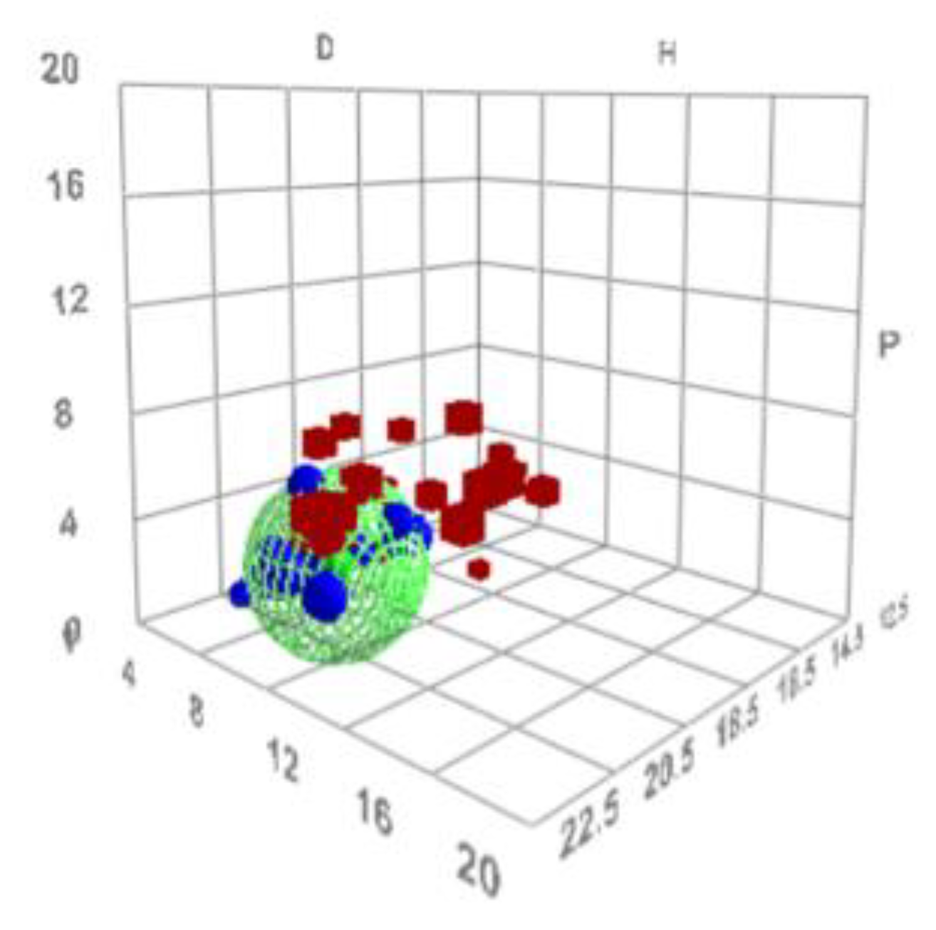
The calculations of the HSP values for N2200 resulted in δD = 18.4, δP = 0.7, δH = 2.3, and R0 = 3.9, and core values of ±[0.15, 0.50, 0.35]. From these values, it is possible to present the solubility of N2200 as a sphere in Hansen space, as seen in Figure 4.
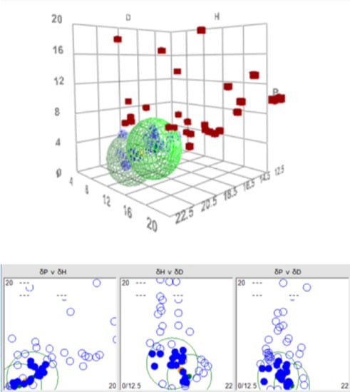
Using the HSP values for TQ1 determined by Holmes et al. [4], i.e., δD = 17.5, δP = 4.0, δH = 3.8, and R0 = 4.8, makes it possible to make a similar solubility sphere for this polymer. Putting these two spheres into the same three-dimensional graphical representation in Hansen space, as seen in Figure 5, shows an overlap region of the two spheres, the so-called junction. Sometimes, the junction is clearer in the two-dimensional projections, as shown in the lower part of Figure 5. Within this junction volume, it is likely that solvents that will be good for both solutes and thus serves as a good starting point when searching for solvent blends will be found. In this particular case, the center of the junction has the HSP values δD = 17.7, δP = 1.3, and δH = 3.4. This set of parameters was used as a target for modelling solvent blends for the pair TQ1:N2200.
It should be mentioned that the HSP values determined may differ from other HSP values given in the literature. In fact, every set of values are dependent on the actual experimental conditions and, hence, may differ. The general picture, however, will persist, in the sense that the relative weights of δD, δP, and δH will remain.
3.2. Alternative Solvent Blends for TQ1 and N2200
With the target HSP of the junction between TQ1 and N2200, the HSPiP program can be used to model possible solvent blends. A set of ten solvent blends were found with promising HSP and RED values; see Table 4. An illustrative example of a solubility test is shown in Figure 6. The resulting scores of the solubility test are given in Table 4. The four blends being good solvents for N2200, i.e., A, C, E, and F, were tested as solvent blends for TQ1. All blends acted as good solvents, and it was possible to dissolve 10 mg/ml of TQ1 in each of the tested blends. This is also as expected, given the larger R0 for TQ1 as compared to the R0 of N2200. A larger R0 is indicative for a broader range of solvents to act as good solvents.
The shortest distance between N2200 and the solvent blend was found for blends F and G, followed by blend E, while the largest distance was found for blends I and J. Evidently, the Ra does not on its own give a precise picture of the solubility of N2200 in the blends—E and F are good solvents, while G is not as good. This is a demonstration of the fact that the HSP model relies on ideal mixing, which is not the case for all blends. This is also clear when comparing the RED values: All RED values are below 1, but not all blends are good solvents. One should remember that the HSP model assumes spherical solubility in Hansen space, which is not necessarily true. Consequently, one needs to perform the solubility tests to discriminate between the calculated solvent blends.
The remaining test was to dissolve the pair TQ1:N2200 in a weight ratio of 1:1 in the promising solvent blends. All four solvent blends turned out to dissolve the two solutes up to a total concentration of 10 mg/ml. It should be pointed out that some of the blends had a very high viscosity, even at 50 °C, making them less promising for applications.
3.3. TQ1 and N2200 Film Morphology
Blend films, with the TQ1:N2200 weight ratio of either 1:1 or 2:1, were spun on glass substrates from the solvent blends A, C, E, and F, as well as from chloroform, a solvent known to be good for both TQ1 and N2200. The dried and thermally annealed films’ morphologies were characterized by AFM measurements; see Figure 7. The TQ1:N2200 blend films do not show strong phase separation in any case, even if there is slightly more structure found in the film spun from chloroform. The reason for this can be sought in several parameters. First, the viscosities of the solvent blends are remarkably higher than that of chloroform, strongly influencing the liquid film deposition on the glass substrate. Second, the films spun from blend solvents are all pre-heated at 250 °C for 1 minute before thermal annealing, while the film spun from chloroform was not pre-heated. This extra annealing, when some solvent is still present, most probably will have an influence on the morphology of the films from solvent blends.
Taking these differences into account, we conclude that the solvent blends, modelled by the HSPiP program, yields thin blend films with similar morphologies to what is found when the film is prepared from a solution with a frequently used solvent. This shows that the HSP model and the HSPiP is a suitable tool for a preliminary screening of solvent and solvent blend possibilities, saving much time for experimental work.
4. Conclusions
We have shown that the Hansen Solubility Parameters and the program Hansen Solvent Parameters in Practice can be used to successfully model possible solvent blends of two polymers, relevant for organic solar cells, i.e., the electron donor TQ1 and the electron acceptor N2200.
From solubility experiments, the HSP parameters δD, δP, δH, R0, Ra, and RED could be determined for N2200. Together with reported parameters for TQ1, the solubility spheres’ junction could be determined and used for solvent blend modelling.
Less harmful solvents can be used to yield similar film morphologies as those obtained with more common, halogenated and/or aromatic, solvents.
In order to undertake a possible forthcoming investigation on solar cell devices produced from new solvent blends, more experimental work is needed to increase the understanding of the role of the solution chemistry in these systems. For instance, blends of three solvents remain to be modelled and investigated, and optical microscopy could be used to monitor the prepared films on a larger scale, i.e., 0.1–1 mm.
Author Contributions
Conceptualization, J.v.S. and I.J.; methodology, J.v.S. I.J, and L.L; validation, J.v.S, I.J., and L.L.; formal analysis, J.v.S. and I.J.; investigation, I.J. and L.L.; writing, J.v.S., I.J., and L.L.; project administration, J.V.S.; fundning acquisition, J.v.S.
Funding
This research was funded by the Swedish National Space Agency, grant number 185/17, and the Knut och Alice Wallenbergs Stiftelse, grant number 2016.0059.
Acknowledgments
This article/communication is a contribution from the SOLA consortium, a KAW funded research consortium with participants from Karlstad University, Chalmers University of Technology, Lund University, and Linköping University. The authors acknowledge the helpful experimental work performed by Brant Tournoy, a visiting exchange student from University College Leuven-Limburg, Leuven, Belgium, under the Erasmus+ scheme of the European Union. The authors thank Ellen Moons, Karlstad University, Karlstad, Sweden, and Natalie Holmes, University of Newcastle, Callaghan, Australia, for valuable discussions. Mikael Andersén and Leif Ericsson (Karlstad University) are acknowledged for valuable discussions and technical support. Lisa Lundin performed her contribution as her degree thesis project.
Conflicts of Interest
The authors declare no conflict of interest.
References
- Sharma, A.; Pan, X.; Bjuggren, J.M.; Gedefaw, D.; Xu, X.; Kroon, R.; Wang, E.; Campbell, J.A.; Lewis, D.A.; Andersson, M.R. Probing the Relationship between Molecular structures, Thermal Transitions, and Morphology in Polymer Semiconductors Using a Woven Glass-Mesh-Based DMTA Technique. Chem. Mater. 2019, 31, 6740–6749. [Google Scholar] [CrossRef]
- Zhu, J.; Liu, Q.; Li, D.; Xiao, Z.; Chen, Y.; Hua, Y.; Yang, S.; Ding, L. A Wide-Band Gap Copolymer Donor for Efficient Fullerene-Free Solar Cells. ACS Omega 2019, 4, 14800–14804. [Google Scholar] [CrossRef] [PubMed]
- Uranbileg, N.; Gao, C.; Yang, C.; Bao, X.; Han, L.; Yang, R. Amorphous electron donros with controllable morphology for non-fullerene polymer solar cells. J. Mater. Chem. C 2019, 7, 10881–10890. [Google Scholar] [CrossRef]
- Holmes, N.P.; Munday, H.; Barr, M.G.; Thomsen, L.; Marcus, M.A.; Kilcoyne, A.L.D.; Fahy, A.; van Stam, J.; Dastoor, P.C.; Moons, E. Unravelling donor-acceptor film morphology formation for environmentally-friendly OPV ink formulations. Green Chem. 2019, 21, 5090–5103. [Google Scholar] [CrossRef]
- Lindqvist, C.; Moons, E.; van Stam, J. Fullerene Aggregation in Thin Films of Polymer Blends for Solar Cell Applications. Materials 2018, 11, 2068. [Google Scholar] [CrossRef] [PubMed]
- Cheng, P.; Li, G.; Zhan, X.; Yang, Y. Next-generation organic photovoltaics based on non-fullerene acceptors. Nat. Photonics 2018, 12, 131–142. [Google Scholar] [CrossRef]
- Cooling, N.A.; Barnes, E.F.; Almyahi, F.; Feron, K.; Al-Mudhafer, M.F.; Al-Ahmad, A.; Vaughan, B.; Andersen, T.R.; Griffith, M.J.; Hart, A.S.; et al. A low-cost mixed fullerene acceptor blend for printed electronics. J. Mater. Chem. A 2016, 4, 10274–10281. [Google Scholar] [CrossRef]
- Blazinic, V.; Ericsson, L.K.E.; Muntean, S.A.; Moons, E. Photo-degradation in air of spin-coated PC60BM and PC70BM films. Synth. Met. 2018, 241, 26–30. [Google Scholar] [CrossRef]
- Morvillo, P.; Bobeico, E.; Esposito, S.; Diana, R. Effect of the active layer thickness on the device performance of polymer solar cells having [60]PCBM and [70]PCBM as electron acceptor. Energy Procedia 2012, 31, 69–73. [Google Scholar] [CrossRef]
- Bruno, A.; Villani, F.; Grimaldi, I.A.; Loffredo, F.; Morvillo, P.; Diana, R.; Haque, S.; Minarini, C. Morphological and spectroscopic characterizations of inkjet-printed poly(3-hexylthiophene-2,5-diyl): Phenyl-C61-butyric acid methyl ester blends for organic solar cell applications. Thin Solid Film. 2014, 560, 14–19. [Google Scholar] [CrossRef]
- Morvillo, P.; Ricciardi, R.; Nenna, G.; Bobeico, E.; Diana, R.; Minarini, C. Elucidating the origin of the improved current output in inverted polymer solar cells. Sol. Energy Mater. Sol. Cells 2016, 152, 51–58. [Google Scholar] [CrossRef]
- Lee, H.; Park, C.; Sin, D.H.; Park, J.H.; Cho, K. Recent Advances in Morphology Optimization for Organic Photovoltaics. Adv. Mater. 2018, 30, 1800453. [Google Scholar] [CrossRef] [PubMed]
- Hansen, C.M. Hansen Solubility Parameters. A User’s Handbook, 2nd ed.; CRC Press: Boca Raton, FL, USA, 2000. [Google Scholar]
- Machui, F.; Brabec, C.J. Solubility, Miscibility, and the Impact on Solid-State Morphology. In Semiconducting Polymer Composites: Principles, Morphologies, Properties and Applications, 1st ed.; Yang, X., Ed.; Wiley-VCH KGaA: Weinheim, Germany, 2012; pp. 1–38. [Google Scholar]
- Miller-Chou, B.A.; Koenig, J.L. A review of polymer dissolution. Prog. Polym. Sci. 2003, 28, 1223–1270. [Google Scholar] [CrossRef]
- Agata, Y.; Yamamoto, H. Determination of Hansen solubility parameters of ionic liquids using double-sphere type of Hansen solubility sphere method. Chem. Phys. 2018, 513, 165–173. [Google Scholar] [CrossRef]
- Zhu, Q.-N.; Wang, Q.; Hu, Y.-B.; Abliz, X. Practical Determination of the Solubility Parameters of 1-Alkyl-3-methylimidazolium Bromide ([CnC1im]Br, n = 5, 6, 7, 8) Ionic Liquids by Inverse Gas Chromatography and the Hansen Solubility Parameter. Molecules 2019, 24, 1346. [Google Scholar] [CrossRef] [PubMed]
- Park, C.-D.; Fleetham, T.A.; Li, J.; Vogt, B.D. High performance bulk-heterojunction organic solar cells fabricated with non-halogenated solvent processing. Org. Electron. 2011, 12, 1465–1470. [Google Scholar] [CrossRef]
- Duong, D.T.; Walker, B.; Lin, J.; Kim, C.; Love, J.; Purushothaman, B.; Anthony, J.E.; Nguyen, T.-C. Molecular Solubility and Hansen Solubility Parameters for the Analysis of Phase Separation in Bulk Heterojunctions. J. Polym. Sci. B Polym. Phys. 2012, 50, 1405–1413. [Google Scholar] [CrossRef]
- Burgués-Ceballos, I.; Machui, F.; Min, J.; Ameri, T.; Voigt, M.M.; Luponosov, Y.N.; Ponomarenko, S.A.; Lacharmoise, P.D.; Campoy-Quiles, M.; Brabec, C.J. Solubility Based Identification of Green Solvents for Small Molecule Organic Solar Cells. Adv. Funct. Mater. 2014, 24, 1449–1457. [Google Scholar] [CrossRef]
- Machui, F.; Langner, S.; Zhu, X.; Abbott, S.; Brabec, C.J. Determination of the P3HT:PCBM solubility parameters via a binary solvent gradient method: Impact of the solubility on the photovoltaic performance. Sol. Energy Mater. Sol. Cells 2012, 100, 138–146. [Google Scholar] [CrossRef]
- Hansen Solubility Parameters in Practice. Available online: https://www.hansen-solubility.com/contact.php (accessed on 1 October 2019).
- Royal Society of Chemistry. GSK Solvent Selection Guie 2009. Available online: http://www.rsc.org/suppdata/gc/c0/c0gc00918k/c0gc00918k.pdf (accessed on 1 October 2019).
Figure 1.
The structure of the donor polymer TQ1.
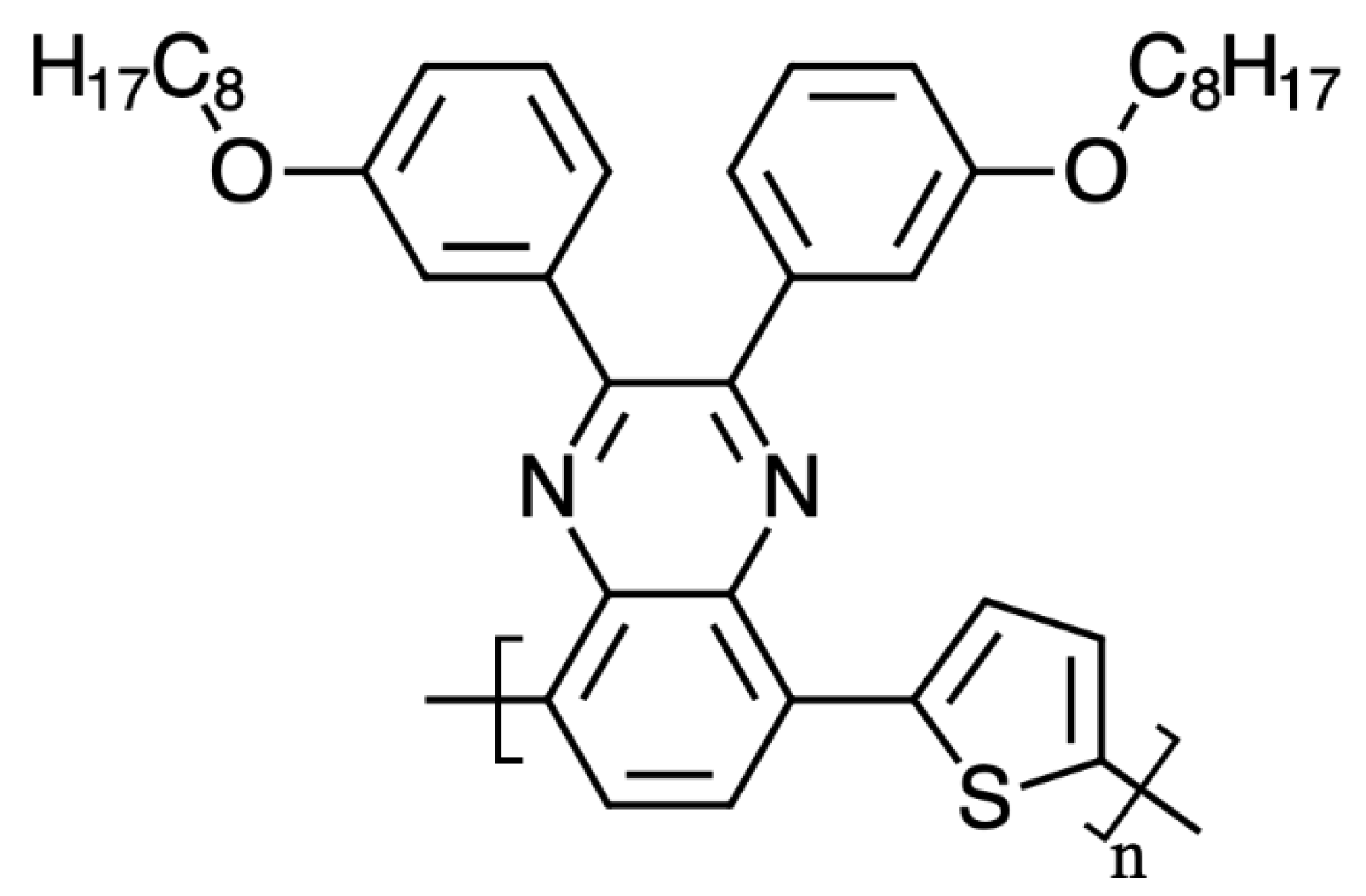
Figure 2.
The structure of the acceptor polymer N2200.
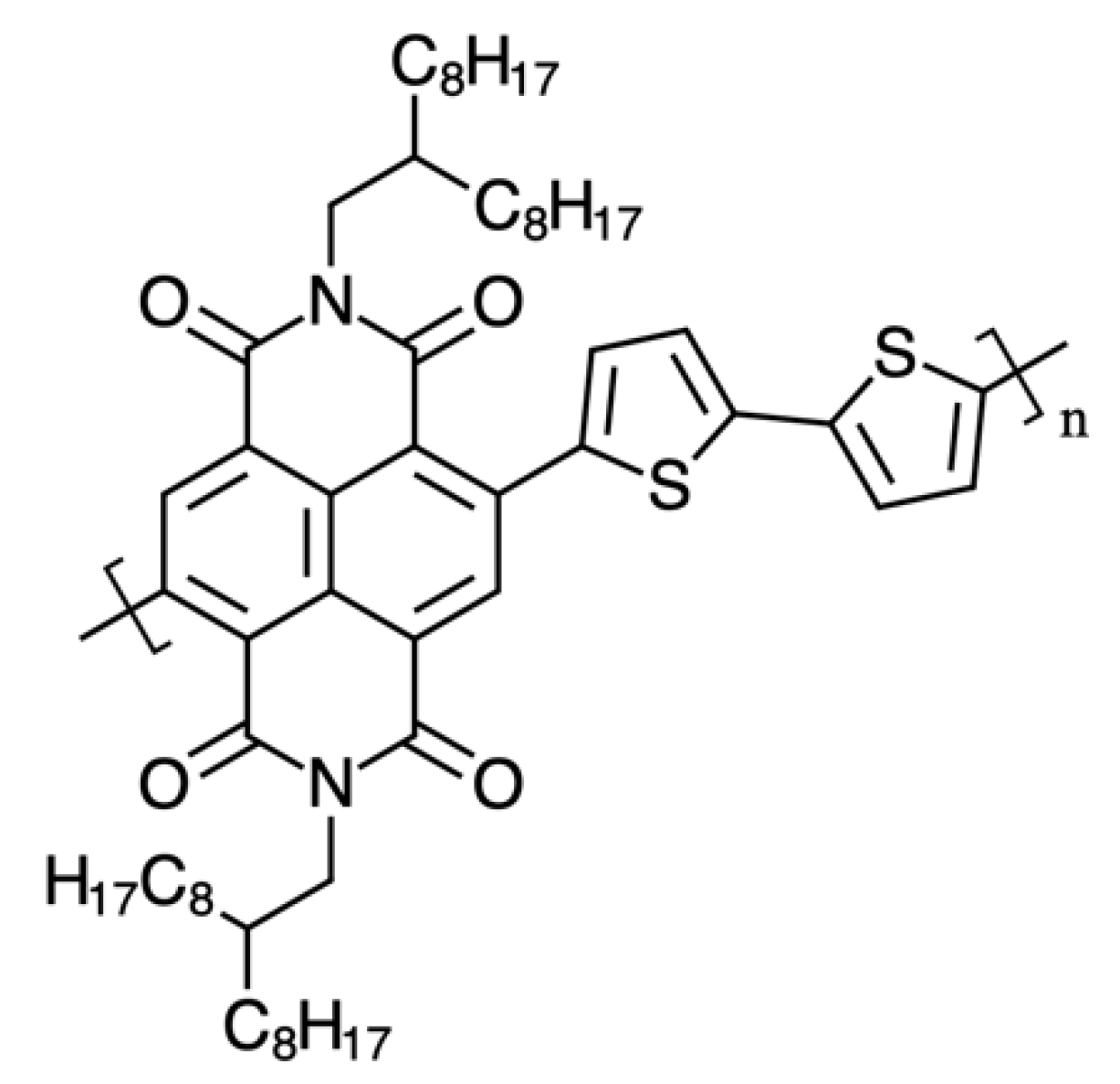
Figure 3.
An illustrative example of how different solubilisation behaviors were scored. The scores are, from left to the right, 1, 2, 3, 4, and 0.
Figure 3.
An illustrative example of how different solubilisation behaviors were scored. The scores are, from left to the right, 1, 2, 3, 4, and 0.

Figure 4.
The solubility sphere for N2200 in Hansen space, as calculated by the HSPiP program. The centre of the sphere has the coordinates of the HSP-values of N2200. Red cubes denote bad solvents and blue spheres good solvents. The axes denoted D, P, and H denote δD, δP, and δH, respectively, in (MPa)1/2.

Figure 5.
A double-sphere graphical representation of the solubilities of N2200 and TQ1. The region where the two spheres overlap, the junction, shows the part of Hansen space where it is likely to find solvents that work for both solutes. The junction is more easily seen in the two-dimensional projection below the three-dimensional Hansen space. The axes denoted D, P, and H denote δD, δP, and δH, respectively, in (MPa)1/2.

Figure 6.
An example of the solubility tests of N2200 in the solvent blends calculated by the HSPiP program, at the initial stage of the test. The blends in the vials are (volume ratio in brackets); A: Toluene/1-methyl naphthalene (62/38), B: Cumene/benzaldehyde (72/28), C: Tetrahydronaphthalene/methyl acetate (88/12), D: Mesitylene/benzaldehyde (65/35), E: Tetrahydronaphthalene/o-xylene (65/35), F: Tetrahydronaphthalene/2-methyl tetrahydrofuran (77/23), G: Tetrahydronaphthalene/isobutyl acetate (85/15), H: Cumene/2-methyl anisole (60/40), I: Ethyl benzene/2-methyl anisole (53/47), J: Cumene/anisole (72/28).
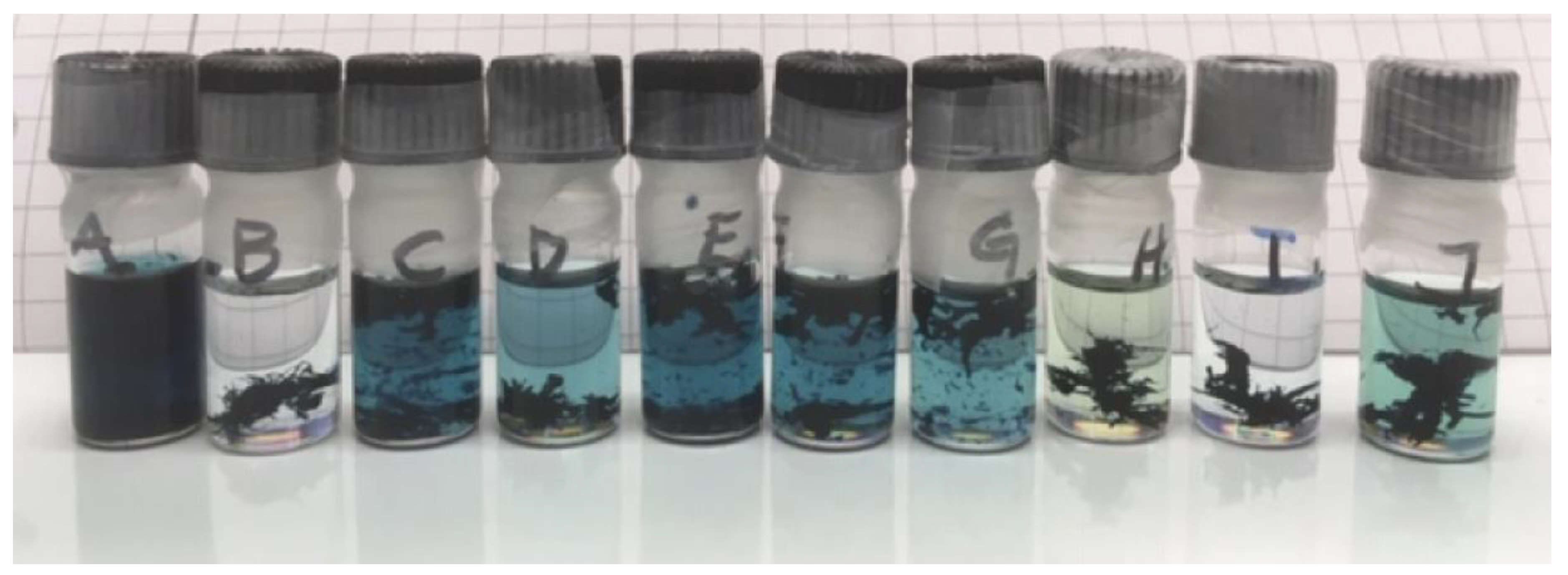
Figure 7.
Atomic force microscopy (AFM) micrographs of blend films spun from various solvents. All films were spun at 1000 rpm and the total solute concentration was 10 mg/ml. All films, except a and b, were pre-heated at 250 °C for 1 minute to complete solvent evaporation. All films were thermally annealed at 120 °C for 10 minutes. The TQ1:N2200 weight ratio was 1:1 in films a, c, e, g, and i, while the ratio was 2:1 in the other films. The solvents are chloroform (a and b), solvent blend A (c and d), solvent blend C (e and f), solvent blend E (g and h), and solvent blend F (i and j).


Table 1.
List of solvents.
| Solvent | Manufacturer | Grade | CAS |
|---|---|---|---|
| 1-Butanol | ACROS | 99% | 71-36-3 |
| 1-Methylnaphthalene | ACROS | 97% | 90-12-0 |
| 1-Octanol | Sigma–Aldrich | ≥99.5% | 111.87-5 |
| 2-Butanol | EMSURE | for analysis | 78-92-2 |
| 2-Methyl Tetrahydrofuran | Sigma–Aldrich | >99.5% | 96-47-9 |
| 2-Propanol (IPA) | VWR Chemicals | AnalaR | 67-63-0 |
| Acetone | VWR Chemicals | 100% | 67-64-1 |
| Amyl Acetate | Sigma–Aldrich | 99% | 628-63-7 |
| Benzaldehyde | Sigma–Aldrich | ≥99.5 | 100-52-7 |
| Chloroform | EMSURE | for analysis | 67-66-3 |
| Cyclohexane | Merck KGaA | ≥99.5% | 110-82-7 |
| Cyclohexanone | Sigma–Aldrich | ≥99% | 108-94-1 |
| Cyclopentyl Methyl Ether | Sigma–Aldrich | ≥99% | 5614-37-9 |
| Dimethyl Formamide (DMF) | Sigma–Aldrich | ≥99% | 68-12-02 |
| Dimethyl Sulfoxide (DMSO) | VWR Chemicals | 99% | 67-68-5 |
| Dipropyl Amine | Sigma–Aldrich | 99% | 142-84-7 |
| Dipropylene Glycol | Sigma–Aldrich | 99% | 25265-71-8 |
| Ethanol | VWR Chemicals | 96% | 64-17-5 |
| Ethyl Acetate | Sigma–Aldrich | ≥99.5% | 141-78-6 |
| Ethyl Benzene | Janssen Chimica | AnalaR Normapur | 100-41-4 |
| Formamide | Sigma–Aldrich | ≥99.5% | 75-12-07 |
| Glycerol | Sigma–Aldrich | ≥99.5% | 56-81-5 |
| Isobutyl Acetate | Sigma–Aldrich | 99% | 110-19-0 |
| Isopropyl Benzene (Cumene) | Sigma–Aldrich | 98% | 98-32-8 |
| Mesitylene | ACROS | 99% extra pure | 108-67-8 |
| Methyl Acetate | Merck KGaA | ≥99% | 79-20-9 |
| Methyl Cyclohexane | ACROS | 99% extra pure | 108-87-2 |
| n-Butyl Acetate | Sigma–Aldrich | ≥99.5% | 123-86-4 |
| N-Methyl Formamide | Sigma–Aldrich | 99% | 123-39-7 |
| o-Xylene | Alfa Aesar | 99% | 95-47-6 |
| Propylene Carbonate | Sigma–Aldrich | 99.7% | 108-32-7 |
| Propylene Glycol | ACROS | 99% | 57-55-6 |
| Tetrahydrofuran (THF) | Sigma–Aldrich | ≥99% | 109-99-9 |
| Tetrahydronaphthalene | Fischer Scientific | Lab. Reagent grade | 119-64-2 |
| Toluene | VWR Chemicals | AnalaR | 108-88-3 |
Table 2.
Solvents used for the solubility tests and their corresponding HSP values.
| Solvent | δD [(MPa)1/2] | δP [(MPa)1/2] | δH [(MPa)1/2] |
|---|---|---|---|
| 1-Butanol | 16.0 | 5.7 | 15.8 |
| 1-Octanol | 16.0 | 5.0 | 11.2 |
| 2-Butanol | 15.8 | 5.7 | 14.5 |
| 2-Methyl Tetrahydrofuran | 16.9 | 5.0 | 4.3 |
| 2-Propanol (IPA) | 15.8 | 6.1 | 16.4 |
| Acetone | 15.5 | 10.4 | 7.0 |
| Amyl Acetate | 15.8 | 3.3 | 6.1 |
| Cyclohexane | 16.8 | 0.0 | 0.2 |
| Cyclohexanone | 17.8 | 8.4 | 5.1 |
| Cyclopentyl Methyl Ether | 16.7 | 4.3 | 4.3 |
| Dimethyl Formamide (DMF) | 17.4 | 13.7 | 11.3 |
| Dimethyl Sulfoxide (DMSO) | 18.4 | 16.4 | 10.2 |
| Dipropyl Amine | 15.3 | 1.4 | 4.1 |
| Dipropylene Glycol | 16.5 | 10.6 | 17.7 |
| Ethanol | 15.8 | 8.8 | 19.4 |
| Ethyl Acetate | 15.8 | 5.3 | 7.2 |
| Ethyl Benzene | 17.8 | 0.6 | 1.4 |
| Formamide | 17.2 | 26.2 | 19.0 |
| Glycerol | 17.4 | 11.3 | 27.2 |
| Isobutyl Acetate | 15.1 | 3.7 | 6.3 |
| Isopropyl Benzene (Cumene) | 18.1 | 1.2 | 1.2 |
| Mesitylene | 18.0 | 0.6 | 0.6 |
| Methyl Acetate | 15.5 | 7.2 | 7.6 |
| Methyl Cyclohexane | 16.0 | 0.0 | 1.0 |
| n-Butyl Acetate | 15.8 | 3.7 | 6.3 |
| N-Methyl Formamide | 17.4 | 18.8 | 15.9 |
| o-Xylene | 18.0 | 2.6 | 2.8 |
| Propylene Carbonate | 20.0 | 18.0 | 4.1 |
| Propylene Glycol | 16.8 | 10.4 | 21.3 |
| Tetrahydrofuran (THF) | 16.8 | 5.7 | 8.0 |
| Tetrahydronaphthalene | 19.6 | 2.0 | 2.9 |
| Toluene | 18.0 | 1.4 | 2.0 |
Table 3.
Solubility scores for N2200, at a concentration of 1.0 mg/ml, in some solvents. Solvents that had a score of 0 in every test are not included in the table. δD, δP, and δH are given in (MPa)1/2.
Table 3.
Solubility scores for N2200, at a concentration of 1.0 mg/ml, in some solvents. Solvents that had a score of 0 in every test are not included in the table. δD, δP, and δH are given in (MPa)1/2.
| Solvent | δD | δP | δH | Score 1 h | Score 24 h | Score 48 h | Score 72 h | Score 96 h |
|---|---|---|---|---|---|---|---|---|
| Ethyl Benzene | 17.8 | 0.6 | 1.4 | 3 | 2 | 2 | 2 | 2 |
| Mesitylene | 18.0 | 0.6 | 0.6 | 3 | 2 | 2 | 2 | 1 |
| o-Xylene | 18.0 | 2.6 | 2.8 | 1 | 1 | 1 | 1 | 1 |
| Tetrahydrofuran (THF) | 16.8 | 5.7 | 8.0 | 4 | 3 | 3 | 3 | 3 |
| Tetrahydronaphthalene | 19.6 | 2.0 | 2.9 | 2 | 1 | 1 | 1 | 1 |
| Toluene | 18.0 | 1.4 | 2.0 | 2 | 2 | 2 | 2 | 2 |
Table 4.
Solvent blends for N2200. The blend ratio is given as volume percentage. The solubility tests were performed for 24 hours at 50 °C. First, the lowest concentration was tested, and subsequently the concentration was increased for good solvent blends. δD, δP, and δH are given in (MPa)1/2.
Table 4.
Solvent blends for N2200. The blend ratio is given as volume percentage. The solubility tests were performed for 24 hours at 50 °C. First, the lowest concentration was tested, and subsequently the concentration was increased for good solvent blends. δD, δP, and δH are given in (MPa)1/2.
| Test # | Solvent Blend | V% | Ra | RED | δD | δP | δH | Score | Score | Score |
|---|---|---|---|---|---|---|---|---|---|---|
| mg/ml | mg/ml | mg/ml | ||||||||
| 1.0 | 5.0 | 10.0 | ||||||||
| A | Toluene | 62.0 | 1.2 | 0.69 | 18.6 | 1.3 | 2.0 | 1 | 1 | 1 |
| 1-Methyl Naphthalene | 38.0 | |||||||||
| B | Isopropyl Benzene (Cumene) | 72.0 | 1.1 | 0.64 | 18.5 | 2.9 | 2.3 | 3 | ||
| Benzaldehyde | 28.0 | |||||||||
| C | Tetrahydronaphthalene | 88.0 | 0.9 | 0.52 | 19.1 | 2.6 | 3.5 | 1 | 1 | 1 |
| Methyl Acetate | 12.0 | |||||||||
| D | Mesitylene | 65.0 | 1.1 | 0.68 | 18.5 | 3.0 | 2.2 | 3 | ||
| Benzaldehyde | 35.0 | |||||||||
| E | Tetrahydronaphthalene | 65.0 | 0.7 | 0.42 | 19.0 | 2.7 | 3.2 | 1 | 1 | 1 |
| o-Xylene | 35.0 | |||||||||
| F | Tetrahydronaphthalene | 77.0 | 0.6 | 0.36 | 18.4 | 2.6 | 2.0 | 1 | 1 | 1 |
| 2-Methyl Tetrahydrofuran | 23.0 | |||||||||
| G | Tetrahydronaphthalene | 85.0 | 0.6 | 0.34 | 18.9 | 2.3 | 3.4 | 2 | ||
| Isobutyl Acetate | 15.0 | |||||||||
| H | Isopropyl Benzene (Cumene) | 60.0 | 1.3 | 0.77 | 18.2 | 2.6 | 2.6 | 3 | ||
| 2-Methyl Anisole | 40.0 | |||||||||
| I | Ethyl Benzene | 53.0 | 1.6 | 0.92 | 18.0 | 2.5 | 3.0 | 3 | ||
| 2-Methyl Anisole | 47.0 | |||||||||
| J | Isopropyl Benzene (Cumene) | 72.0 | 1.6 | 0.93 | 18.0 | 2.1 | 2.8 | 2 | ||
| Anisole | 28.0 |
© 2019 by the authors. Licensee MDPI, Basel, Switzerland. This article is an open access article distributed under the terms and conditions of the Creative Commons Attribution (CC BY) license (http://creativecommons.org/licenses/by/4.0/).
Share and Cite
MDPI and ACS Style
Jalan, I.; Lundin, L.; van Stam, J. Using Solubility Parameters to Model More Environmentally Friendly Solvent Blends for Organic Solar Cell Active Layers. Materials 2019, 12, 3889. https://doi.org/10.3390/ma12233889
AMA Style
Jalan I, Lundin L, van Stam J. Using Solubility Parameters to Model More Environmentally Friendly Solvent Blends for Organic Solar Cell Active Layers. Materials. 2019; 12(23):3889. https://doi.org/10.3390/ma12233889
Chicago/Turabian StyleJalan, Ishita, Lisa Lundin, and Jan van Stam. 2019. "Using Solubility Parameters to Model More Environmentally Friendly Solvent Blends for Organic Solar Cell Active Layers" Materials 12, no. 23: 3889. https://doi.org/10.3390/ma12233889
Note that from the first issue of 2016, this journal uses article numbers instead of page numbers. See further details here.