
Determining Surface Topography of a Dressed Grinding Wheel Using Bio-Inspired DNA-Based Computing


1
Division of Mechanical and Electrical Engineering, Kitami Institute of Technology, 165 Koen-cho, Kitami 090-8507, Japan
2
Department of Chemical, Materials and Industrial Production Engineering, University of Naples Federico II, Piazzale Tecchio 80, 80125 Naples, Italy
*
Author to whom correspondence should be addressed.
Materials 2021, 14(8), 1899; https://doi.org/10.3390/ma14081899
Submission received: 13 March 2021
/
Revised: 3 April 2021
/
Accepted: 5 April 2021
/
Published: 11 April 2021
(This article belongs to the Special Issue Special Issue of Manufacturing Engineering Society-2020 (SIMES-2020))
Abstract
:Grinding is commonly used for machining parts made of hard or brittle materials with the intent of ensuring a better surface finish. The material removal ability of a grinding wheel depends on whether the wheel surface is populated with a sufficiently high number of randomly distributed active abrasive grains. This condition is ensured by performing dressing operations at regular time intervals. The effectiveness of a dressing operation is determined by measuring the surface topography of the wheel (regions and their distributions on the grinding wheel work surface where the active abrasive grains reside). In many cases, image processing methods are employed to determine the surface topography. However, such procedures must be able to remove the regions where the abrasive grains do not reside while keeping, at the same time, the regions where the abrasive grains reside. Thus, special kinds of image processing techniques are needed to distinguish the non-grain regions from the grain regions, which requires a heavy computing load and long duration. As an alternative, in the framework of the “Biologicalisation in Manufacturing” paradigm, this study employs a bio-inspiration-based computing method known as DNA-based computing (DBC). It is shown that DBC can eliminate non-grain regions while keeping grain regions with significantly lower computational effort and time. On a surface of size 706.5 μm in the circumferential direction and 530 μm in the width direction, there are about 7000 potential regions where grains might reside, as the image processing results exhibit. After performing DBC, this number is reduced to about 300 (representing a realistic estimate). Thus, the outcomes of this study can help develop an intelligent image processing system to optimize dressing operations and thereby, grinding operations.
1. Introduction
Grinding is commonly used to machine workpieces made of hard or brittle materials with the intent of ensuring a better surface finish. In grinding, the shape of the grinding wheel and the randomly distributed abrasive grain trajectories are projected onto the workpiece surface [1]. Thus, the cutting-edge density of the abrasive grains, the number of protrusions of the grains, and the continuous cutting-edge intervals affect the abrasive grain trajectories and thereby, the surface finish [2,3,4]. The critical aspect is that the material removal ability of the abrasive grains deteriorates with time. Dressing and truing operations are performed at regular time intervals to restore the abrasive grains’ material removal ability. Various methods have been introduced so far to perform truing and dressing [5,6,7]. The effectiveness of truing and dressing operations is determined by quantifying wheel surface topography by identifying the regions and their distributions where the active abrasive grains reside.
Both analytical and experimental studies have been carried out to determine the surface topography of the grinding wheel. Numerous studies have been carried out to theoretically analyze the surface topography of the dressed grinding wheel and the properties of the finished surface [8,9,10]. Besides theoretical analysis, experimental and hybrid analyses have been a popular approach. In this regard, stylus-based measurements have largely been used. Matsui et al. [11] conducted a theoretical analysis and an experimental study of abrasive grain cutting-edge density for both the conical stylus and knife-edge stylus. One of the drawbacks of this approach is that the measurement results depend on the shape of the stylus. In addition to stylus-based measurements, non-contact measurements have also been used. Shoji et al. [12] measured the amount of protrusion of abrasive grains by stereo-photography and investigated the effect of this amount on grinding performance. Laser-based, non-contact measurements can be used to obtain the distribution of the grinding wheel outer surface heights with high accuracy [13,14,15]. Furthermore, the surface topography of the grinding wheel can be analyzed by various image processing methods [16,17,18,19,20,21,22,23,24]. In this case, the images of the grinding wheel work surface are prepared by pre-processing before the actual processing phase. These methods can measure a wide surface area quickly and quantify the grinding wheel surface conditions more realistically. For example, consider the work described in Hosokawa et al. [16]. In this article, the grinding wheel surface image was prepared in three steps: preprocessing of a color image, binary conversion, and main processing of a micro-chromatic image. The binary conversion was performed in the regions of abrasive grain and worn-flat areas with the aid of hue histograms, saturation histograms, and brilliance histograms. For example, consider some selected recent studies. Feng and Chen [17] showed that manual adjustment was required during the image processing of a grinding wheel surface, ensuring the right detection of the regions where the abrasive grains reside. Kawashita et al. [18] used an image processing system to determine a targeted abrasive grain’s wear due to the continuation of a grinding process. They extracted abrasive grain height information by processing the grinding wheel work surface using hue, saturation, and brilliance histograms. Abidi et al. [19] showed a digital image processing technique using the K-cluster iteration method to determine the abrasive and non-abrasive regions on a grinding wheel surface. Scanning electron microscope (SEM) images are also used for the sake of comparison. Kawashita et al. [20] developed an imaging technique wherein two light sources (ultraviolet and visible light sources) were used to take images of a grinding wheel surface with diamond abrasives. Kapłonek et al. [21,22,23] performed a series of studies showing the newly developed grinding wheel’s effectiveness by analyzing images of wheel surfaces and images of isolated abrasive grains. The original images were taken by scanning electron microscope (SEM) technology. Afterward, commercially available image processing systems were used to determine the topography of the grinding wheel surface. In topography analysis, the main challenge was to isolate the regions of grains, binders, and cavities in the binders [24]. The authors observed that cavities were also formed in the regions of grains.
However, one of the drawbacks of image processing-based topography analysis is that the underlying image processing method must remove the regions where the abrasive grains do not reside while maintaining at the same time the regions where the abrasive grains reside. Thus, innovative image processing techniques are needed to allow for effective distinction between non-grain regions and grain regions while simultaneously reducing the heavy computing load and time-consuming duration.
In the framework of the emerging paradigm of “Biologicalisation: Biological Transformation in Manufacturing” [24,25,26,27,28], the basic hypothesis is that future biologicalized manufacturing systems will develop along the three directions of (a) bio-inspiration, (b) bio-integration, and (c) bio-intelligence [28]. With reference to this assumption, the present paper aims to embrace the bio-inspiration manufacturing scheme defined as “Bio-inspired manufacturing is realized by transferring concepts concerning principles, functions, structures and/or solutions from the biosphere to the manufacturing technosphere” [28]. Within this concept, for overcoming the limits of current image processing-based topography analysis methods, this study presents a bio-inspiration based computing methodology, known as DNA-based computing (DBC) [29], with a focus on DBC’s effectiveness in helping remove non-grain regions while maintaining grain regions with a significantly reduced amount of computational effort and time.
After the introduction, this article is organized in the following sections: Section 2 presents the dressing conditions and pre-processing of the grinding wheel surface images. Section 3 describes the way DBC is performed on the pre-processed images to eliminate image regions that are not significant for surface topography determination. Section 4 presents the results of the DBC-driven image processing for grinding wheel surface topography determination. It also shows the relationship between dressing conditions and the distributions of active abrasive grains and discusses the implications of this study. Section 5 presents the concluding remarks of this research work.
2. Image Data Preparation
Vitrified CBN grinding wheels (BN140M100V) were used for surface topography analysis. The grinding wheel, dresser specifications, dressing conditions (rotational speeds, velocity ratios, depth of cuts, and feed rates of dressing operations), and coolant type are listed in Table 1. The illustrative descriptions of dressing operations and relevant conditions can be found in [8,9,10]. As can be seen in Figure 1, the photographic images and surface height information of the grinding wheel surfaces under different dressing conditions are obtained using a short wavelength laser microscope (specification VK-9700, Keyence Corp., Osaka, Japan). The magnification factor was 20. For photographic imaging, the resolution of the data was 2048 pixels by 1536 pixels for surface size 706.5 μm in the circumferential direction and 530 μm in the width direction of the grinding wheel, respectively. Thus, unit pixel means here a 345 nm by 345 nm area. Figure 2 shows a typical image of the vicinity of an active abrasive grain. The white region marked as an active abrasive grain is the target area that must be distinguished from the other areas during the image processing-based topography determination process.
The color information of a pixel in a given image, denoted as R ∈ [0, 255], G ∈ [0, 255], B ∈ [0, 255], can be used to produce a grayscale image using the following formulae.
In Equations (1) and (2), Y ∈ [0, 255] is the numerical value of a pixel in the image, and the weights are wR = 0.2989, wG = 0.5870, and wB = 0.1140. A gray scale image can be converted into a binary image. In this case, a threshold a ∈ [0, 254] can be set to perform the following calculation for each pixel.
Thus, a pixel is represented by either 0 or 1 as Z ∈ {0, 1}. Since a binary image produced from a height image is less informative compared to the latter, as shown in Figure 3, the binary images created from photographic images are considered for further analysis. In addition, the threshold a is a critical parameter, as shown in Figure 3. The white regions (corresponding to 1 s) represent the regions where the abrasive grains might reside. From visual inspection, it is evident that the binary images extracted from the photographic images corresponding to a = 150 exhibit a realistic proportion of white and black areas. To be more specific, consider the case shown in Figure 4. This figure shows both photography- and height-based binary images for VR = +0.9 and a = 50, 100, 150, and 200, respectively. Other than a = 150, the white areas in the binary images do not correctly reflect the existence of the active abrasive grains. Accordingly, the binary images extracted from photographic images corresponding to a = 150 are utilized for grinding wheel surface topography analysis.
3. DNA-Based Computing (DBC)
Within the bio-inspiration scheme of “Biologicalisation in Manufacturing” [28], the bio-inspired DNA-based computing (DBC) method [29,30] is utilized according to the central dogma of molecular biology: Once the information of the DNA (sequence of four elements, A, C, G, and T) is passed to a protein (sequence of twenty elements (amino acid), it does not return [31]. This phenomenon is schematically illustrated in Figure 5. As a result, an information content increase takes place (see [32] for the details). Thus, DBC can help solve complex computational problems associated with intelligent manufacturing. It can help detect abnormalities in a manufacturing process even though there is a shortage of relevant data to make the decision [30]. It can identify similarities among tool wear images extracted from the same manufacturing process at different machining times [32,33]. It can help identify the similarity between chaotic time series of surface roughness, ensuring simulation process validity for intelligent machining. Furthermore, it can be used to construct digital twins [34]. Most importantly, it can identify complex boundaries in binary images for geometric modeling [29].
The DBC method is schematically illustrated in Figure 6. As can be seen in the figure, DBC provides several decision rules for solving a given problem. To this purpose, first, the problem-relevant information is prepared. For this case, the problem-relevant information is a piece of a binary image extracted from a photographic image for a = 150. The problem-relevant information is transformed into DNA (a sequence or array of A, C, G, and T), as found in biological organisms. For this, user-defined DNA synthesizing rules are needed. The rules can be reset as many times as desired. Different DNA sequences or arrays can be produced by changing the problem-relevant information. The DNA sequences or arrays can be integrated to produce mRNA. Every three pairs of codes (denoted as codons) can be translated to form a protein (a sequence or array of amino acids). In this case, the universal genetic codes (see Table 2) that translate codons to corresponding amino acids are used.
The formulations used to perform DBC on the binary images are described as follows: Let B(0) be the binary image produced as described in Section 2. The binary image can be processed to produce arrays C(0), adding padding as preferred. The padded array C(0) can be transformed into A(1), B(1), and C(1). The process continues, as schematically illustrated in Figure 7.
Thus, the following formulations hold:
In Equation (5), b, n, m, l, and k are user-defined parameters. In this study, three arrays denoted as B(1), B(3), and B(5) are produced for all m = n = 5. The modified binary arrays are compared with the original ones B(0) to produce three different DNA arrays denoted as D(1), D(3), and D(5). In doing so, different formulations can be employed. In this study, two formulations were used. One of the formulations was defined as the ACTG rule. The other was defined as the ACGT rule. The ACTG and ACGT rules, respectively, are shown below.
In Equations (6) and (7), x ∈ {1, 3, 5}. Figure 6 shows an example of forming D(1) using the ACTG rule. The elements of D(x) are synthesized to create mRNA. Thus, the following formulation holds.
The elements Rk,l are translated into Protk,l ∈ {I, L, V, F, M, C, A, G, P, T, S, Y, W, Q, N, H, E, D, K, R, X}. The translation rules are listed in Table 3 and are based on the genetic codes shown in Table 2.
The existence of a specific amino acid can be shown as a white region. In this way, the protein array is transformed into a binary image. These images can be studied to solve grinding wheel surface topology problems. For example, Figure 8 shows the distributions of amino acids denoted as F, P, Q, K, V, and G in a protein where the DNA is produced using the ACTG rule. The other amino acids (not shown in Figure 8) are absent or rarely present in the protein array. As can be seen in Figure 8, the amino acid denoted as G shows relatively large and noise-free white regions distributed randomly. The corresponding binary image is thus significant for surface topography assessment. On the other hand, Figure 9 shows the distributions of amino acids denoted as F, L, W, P, K, and G in a protein array where the DNA is produced using the ACGT rule. Other amino acids (not shown in Figure 9) are absent or rarely present in the protein array. As can be seen in Figure 9, the amino acid denoted as F shows relatively large and noise-free white regions. The corresponding binary image is thus significant for surface topography assessment.
4. Results and Discussion
The DBC method helped eliminate irrelevant areas for topography assessment. One example of this procedure is shown below. Figure 10 shows three sets of binary images, wherein each set consists of two images. The images under the script “Original” are the original images B(0). The images under the script “ACTG rule” show the areas (white areas) where the amino acid denoted as G resided. These images were produced using the ACTG rule. On the other hand, the images under the script “ACGT rule” show the areas (white areas) where the amino acid denoted as F resided. These images were produced using the ACGT rule. The images with red dots show the centers of the white areas. As can be seen in Figure 10, the small white regions disappeared in DBC-generated binary images, whereas the large white regions remained as they were. This means that DBC helped perform Boolean transformation between useful and non-useful regions in binary images. Therefore, binary images were obtained by performing DBC according to the ACGT rule, wherein the white area represents Fs after performing DBC according to the ACGT rule. Figure 11 shows the number of centers of images, like those shown in Figure 10, for different values of velocity ratio (VR, see Table 1) which is a critical dressing parameter [8,9,10]. The probability of having more active abrasive grains was high when VR = [0.3, 0.9]. This helped optimize the dressing process more effectively. Out of the two rules, the ACGT rule helped reduce small white areas. Thus, this rule could determine the number of active abrasive grains and their distributions.
Appendix A reports the images based on which the plot in Figure 11 is constructed. As can be seen in Figure 11, on a surface of size 706.5 μm in the circumferential direction and 530 μm in the width direction (see Table 1), there were about 7000 potential regions of possible grain residence; however, most regions were very small and did not qualify for topography determination. After performing DBC, this number was notably reduced to about 300 (which was a realistic estimate), showing that the noise which was not possible to eliminate via binary image pre-processing could be easily removed with the aid of DBC. The process is fast and can be very easily automated using commercially available image processing tools (e.g., MATLAB™ image processing toolbox). Thus, the outcomes of this study can help develop a bio-inspired, intelligent image processing system to optimize dressing operations and thereby, grinding operations, as schematically illustrated in Figure 12.
5. Concluding Remarks
Image processing is often employed to determine the surface topography of a dressed grinding wheel. The underlying surface topography determination process requires successful removal of regions where active abrasive grains do not reside while keeping, at the same time, the regions where active abrasive grains do reside. This results in heavy and time-consuming computation, as other authors reported. In this regard, bio-inspired DBC provides a pragmatic solution, as demonstrated in this article. It was found that on a grinding wheel surface of size 706.5 mm in the circumferential direction and 530 mm in the width direction, there were about 7000 potential regions of possible grain residence, wherein most of the regions were very small and did not qualify for topography determination. After performing DBC, this number was reduced to about 300 (which was a realistic estimate). Thus, the noise reduction ability of DBC worked well for the case of grinding wheel surface topography determination.
As enhanced “Biologicalisation in Manufacturing,” based on the convergence between biology and advanced manufacturing technology, is one of the emerging paradigms of next-generation manufacturing systems, effective, bio-inspired computing methods are greatly solicited. The presented DBC method is a contribution toward bio-inspiration endeavors in future biologicalized manufacturing systems. In this study, DBC could effortlessly eliminate unwanted image regions, represented by random distribution in binary images, while keeping, at the same time, the desired regions. Thus, DBC is particularly suitable for Boolean operations performed on binary images exhibiting complex characteristics. As a result, the DBC methodology can be used in grinding wheel surface topography determination as well as in other image processing problems relevant for intelligent manufacturing technology and systems.
Author Contributions
Conceptualization, A.K., R.T., A.S.U., K.I. and T.S.; methodology, A.K., R.T., A.S.U. and K.I.; software, A.K., A.S.U. and K.I.; validation, A.K., R.T. and A.S.U.; formal analysis, R.T. and K.I.; resources, A.K., R.T., and A.S.U.; data curation, A.K., R.T. and A.S.U.; writing—original draft preparation, R.T. and A.S.U.; writing—review and editing, A.K., R.T., A.S.U., and T.S.; visualization, A.K., R.T., A.S.U. and K.I.; supervision, R.T. and A.S.U. All authors have read and agreed to the published version of the manuscript.
Funding
This research received no external funding.
Institutional Review Board Statement
Not Applicable.
Informed Consent Statement
Not Applicable.
Data Availability Statement
Data are contained within this article.
Conflicts of Interest
The authors declare no conflict of interest.
Appendix A. DBC-Driven Image Processing Results
This Appendix reports the datasets corresponding to Figure 11. The datasets are shown in Table A1, Table A2, Table A3, Table A4, Table A5, Table A6, Table A7, Table A8, Table A9 and Table A10 for VR = +0.3, +0.5, +0.9, +1.1, +1.4, −0.3, −0.5, −0.9, −1.1, and −1.4, respectively. In each table, three sets of images are shown where each set consists of two images. In each table, the left-hand-side image in the first set of images is an “Original” image, i.e., the image before performing DBC; the right-hand-side image depicts the centers of the white regions by red dots on the left-hand side image. The left-hand-side image in the second set of images shows the ACTG rule generated image; the right-hand-side image depicts the centers of the white regions by red dots on the left-hand side image. The left-hand-side image in the last set of images shows the ACGT rule generated image; the right-hand-side image depicts the centers of the white regions by red dots on the left-hand-side image. The numbers of pixels and centers of the corresponding images are also listed in Table A1, Table A2, Table A3, Table A4, Table A5, Table A6, Table A7, Table A8, Table A9 and Table A10.

Table A1.
Images and associated pixels and number of centers corresponding to VR = +0.3.
| VR +0.3 | |
| Original | |
 |  |
| Pixels: 221,678 | Number of Centers: 6291 |
| ACTG Rule | |
 |  |
| Pixels: 89,441 | Number of Centers: 308 |
| ACGT RULE | |
 |  |
| Pixels: 71,525 | Number of Centers: 208 |
Table A2.
Images and associated pixels and number of centers corresponding to VR = +0.5.
| VR +0.5 | |
| Original | |
 |  |
| Pixels: 234,204 | Number of Centers: 6186 |
| ACTG RULE | |
 |  |
| Pixels: 95,704 | Number of Centers: 314 |
| ACGT RULE | |
 |  |
| Pixels: 78,923 | Number of Centers: 191 |
Table A3.
Images and associated pixels and number of centers corresponding to VR = +0.9.
| VR +0.9 | |
| Original | |
 |  |
| Pixels: 271,502 | Number of Centers: 5603 |
| ACTG RULE | |
 |  |
| Pixels: 143,299 | Number of Centers: 310 |
| ACGT RULE | |
 |  |
| Pixels: 125,277 | Number of Centers: 213 |
Table A4.
Images and associated pixels and number of centers corresponding to VR = +1.1.
| VR +1.1 | |
| Original | |
 |  |
| Pixels: 233,675 | Number of Centers: 5561 |
| ACTG RULE | |
 |  |
| Pixels: 111,833 | Number of Centers: 277 |
| ACGT RULE | |
 |  |
| Pixels: 95,118 | Number of Centers: 189 |
Table A5.
Images and associated pixels and number of centers corresponding to VR = +1.4.
| VR +1.4 | |
| Original | |
 |  |
| Pixels: 230,005 | Number of Centers: 6192 |
| ACTG RULE | |
 |  |
| Pixels: 98,949 | Number of Centers: 320 |
| ACGT RULE | |
 |  |
| Pixels: 80,943 | Number of Centers: 197 |
Table A6.
Images and associated pixels and number of centers corresponding to VR = −0.3.
| VR −0.3 | |
| Original | |
 |  |
| Pixels: 203,794 | Number of Centers: 5717 |
| ACTG Rule Generated | |
 |  |
| Pixels: 91,432 | Number of Centers: 213 |
| ACGT Rule Generated | |
 |  |
| Pixels: 78,763 | Number of Centers: 143 |
Table A7.
Images and associated pixels and number of centers corresponding to VR = −0.5.
| VR −0.5 | |
| Original | |
 |  |
| Pixels: 193,887 | Number of Centers: 5487 |
| ACTG Rule Generated | |
 |  |
| Pixels: 76,038 | Number of Centers: 253 |
| ACGT Rule Generated | |
 |  |
| Pixels: 61,240 | Number of Centers: 148 |
Table A8.
Images and associated pixels and number of centers corresponding to VR = −0.9.
| VR −0.9 | |
| Original | |
 |  |
| Pixels: 178,438 | Number of Centers: 4955 |
| ACTG Rule Generated | |
 |  |
| Pixels: 69,037 | Number of Centers: 234 |
| ACGT Rule Generated | |
 |  |
| Pixels: 54,337 | Number of Centers: 157 |
Table A9.
Images and associated pixels and number of centers corresponding to VR = −1.1.
| VR −1.1 | |
| Original | |
 |  |
| Pixels: 211,118 | Number of Centers: 5876 |
| ACTG Rule Generated | |
 |  |
| Pixels: 83,910 | Number of Centers: 306 |
| ACGT Rule Generated | |
 |  |
| Pixels: 66,292 | Number of Centers: 192 |
Table A10.
Images and associated pixels and number of centers corresponding to VR = −1.4.
| VR −1.4 | |
| Original | |
 |  |
| Pixels: 215,721 | Number of Centers: 6256 |
| ACTG Rule Generated | |
 |  |
| Pixels: 92,682 | Number of Centers: 268 |
| ACGT Rule Generated | |
 |  |
| Pixels: 77,676 | Number of Centers: 167 |
References
- Malkin, S. Grinding Technology: Theory and Applications of Machining with Abrasives; Ellis Horwood Limited: Chichester, UK, 1989; pp. 79–106. [Google Scholar]
- Tsuwa, H. On the Behaviors of Abrasive Grains in Grinding Process (Part 2)—Successive Cutting-edge Spacing. J. Jpn. Soc. Precis. Eng. 1961, 27, 409–413. [Google Scholar] [CrossRef] [Green Version]
- Tsuwa, H. On the Behaviors of Abrasive Grains in Grinding Process (Part 3)—Cutting-edge Ratio. J. Jpn. Soc. Precis. Eng. 1971, 27, 414–420. [Google Scholar] [CrossRef]
- Ullah, A.M.M.S.; Caggiano, A.; Kubo, A.; Chowdhury, M.A.K. Elucidating Grinding Mechanism by Theoretical and Experimental Investigations. Materials 2018, 11, 274. [Google Scholar] [CrossRef] [PubMed] [Green Version]
- Huang, H. Effects of truing/dressing intensity on truing/dressing efficiency and grinding performance of vitrified diamond wheels. J. Mater. Process. Technol. 2001, 117, 9–14. [Google Scholar] [CrossRef]
- Wegener, K.; Hoffmeister, H.-W.; Karpuschewski, B.; Kuster, F.; Hahmann, W.-C.; Rabiey, M. Conditioning and monitoring of grinding wheels. CIRP Ann. Manuf. Technol. 2011, 60, 757–777. [Google Scholar] [CrossRef]
- Deng, H.; Xu, Z. Dressing methods of super abrasive grinding wheels: A review. J. Manuf. Process. 2019, 45, 46–69. [Google Scholar] [CrossRef]
- Kubo, A.; Chowdhury, M.A.K.; Noda, S.; Tamaki, J.; Ullah, A.M.M.S. Visualization of 3D Topography of Grinding Wheel Surface Dressing by Rotary Diamond Dresser. Adv. Mater. Res. 2013, 797, 751–756. [Google Scholar] [CrossRef]
- Kubo, A.; Ullah, A.M.M.S.; Tamaki, J. Computer-Aided Simulation of Dressing Using Diamond Rotary Dresser and Visualization of Dressing Process. Adv. Mater. Res. 2014, 1017, 592–597. [Google Scholar] [CrossRef]
- Chowdhury, M.A.K.; Kubo, A.; Tamaki, J.; Ullah, A.M.M.S. Computer-aided Simulation of Rotary Diamond Dressing Based on Kinematic Analysis. J. Adv. Mech. Des. Syst. Manuf. 2013, 7, 506–520. [Google Scholar] [CrossRef] [Green Version]
- Matsui, S.; Tamaki, J. Studies on Measuring Method of Wheel Surface Topography—4th Report: Stylus Method. J. Jpn. Soc. Precis. Eng. 1984, 50, 672–678. [Google Scholar] [CrossRef]
- Syoji, K.; Zhou, L.; Matsui, S. Studies on Truing and Dressing of Diamond Wheels—1st Report: The Measurement of Protrusion Height of Abrasive Grains by Using a Stereo Pair and the Influence of Protrusion Height on Grinding Performance. J. Jpn. Soc. Precis. Eng. 1989, 55, 865–870. [Google Scholar] [CrossRef]
- Kakino, Y.; Matubara, A.; Yamaji, I.; Matuda, K.; Nakagawa, H.; Hirogaki, T.; Kita, Y. A Study on Measuring Surface Topography of Grinding Wheel on the Machine—1st Report: Development of Measuring System using a Laser Stylus. J. Jpn. Soc. Precis. Eng. 1997, 63, 228–232. [Google Scholar] [CrossRef] [Green Version]
- Lee, H.S.; Yamada, T.; Uchida, G.; Kobayashi, M. Development of a 3-D Measuring Equipment for Surface Geometries of Grinding Wheel Surfaces. In Proceedings of the ASPE 2006 Annual Meeting, Monterey, CA, USA, 15–20 October 2006. [Google Scholar]
- Uchida, G.; Yamada, T.; Miura, K.; Lee, H.S. Measurement of grinding wheel surface shape by measured focus position recalculation method. J. Jpn. Soc. Abras. Technol. 2020, 64, 140–145. [Google Scholar]
- Hosokawa, A.; Yasui, H.; Kanao, Y.; Sato, K. Characterization of Grinding Wheel Surface by Means of Image Processing—1st Report: Post-process Measurement of Abrasive Grain and Cutting-Edge Distribution on the Wheel Surface. J. Jpn. Soc. Precis. Eng. 1996, 62, 1297–1301. [Google Scholar] [CrossRef] [Green Version]
- Feng, Z.; Chen, X. Image processing of grinding wheel surface. Int. J. Adv. Manuf. Technol. 2007, 32, 452–458. [Google Scholar] [CrossRef]
- Kawashita, T.; Sakaguchi, A.; Matsuo, S.; Shirahama, F. Three-dimensional measurement of wheel surface topography with image processing—2nd Report: Behavior of CBN wheel cutting edges in the grinding process. J. Jpn. Soc. Abras. Technol. 2009, 53, 690–694. [Google Scholar]
- Adibi, H.; Rezaei, S.M.; Sarhan, A.A.D. Grinding wheel loading evaluation using digital image processing. J. Manuf. Sci. Eng. 2014, 136, 1–9. [Google Scholar] [CrossRef]
- Kawashita, T.; Sakaguchi, A.; Ohta, K.; Maeda, J.; Matuo, S.; Nakajima, S.; Toge, N.; Furuno, D.; Shimomura, Y.; Miki, S. Three-dimensional measurement of wheel surface topography with image processing—5th Report: Extraction of diamond abrasive grains using two wavelength band images. J. Jpn. Soc. Abras. Technol. 2017, 61, 551–556. [Google Scholar]
- Kapłonek, W.; Nadolny, K.; Ungureanu, A.; Pimenov, D.Y.; Zieliński, B. SEM-based observations and analysis of the green silicon carbide grinding wheel active surfaces after the graphite and silicone impregnation process. Int. J. Surf. Sci. Eng. 2019, 13, 181. [Google Scholar] [CrossRef]
- Kapłonek, W.; Nadolny, K.; Sutowska, M.; Mia, M.; Pimenov, D.Y.; Gupta, M.K. Experimental Studies on MoS2-Treated Grinding Wheel Active Surface Condition after High-Efficiency Internal Cylindrical Grinding Process of INCONEL® Alloy 718. Micromachines 2019, 10, 255. [Google Scholar] [CrossRef] [Green Version]
- Kapłonek, W.; Nadolny, K.; Rokosz, K.; Marciano, J.; Mia, M.; Pimenov, D.Y.; Kulik, O.; Gupta, M.K. Internal Cylindrical Grinding Process of INCONEL® Alloy 600 Using Grinding Wheels with Sol–Gel Alumina and a Synthetic Organosilicon Polymer-Based Impregnate. Micromachines 2020, 11, 115. [Google Scholar] [CrossRef] [Green Version]
- Bazan, A.; Kawalec, A.; Rydzak, T.; Kubik, P.; Olko, A. Determination of Selected Texture Features on a Single-Layer Grinding Wheel Active Surface for Tracking Their Changes as a Result of Wear. Materials 2020, 14, 6. [Google Scholar] [CrossRef] [PubMed]
- Byrne, G.; Dimitrov, D.; Monostori, L.; Teti, R.; Van Houten, F.; Wertheim, R. Biologicalisation: Biological Transformation in Manufacturing. CIRP J. Manuf. Sci. Technol. 2018, 21, 1–32. [Google Scholar] [CrossRef]
- Neugebauer, R.; Ihlenfeldt, S.; Schließmann, U.; Hellmich, A.; Noack, M. A New Generation of Production with Cyber-Physical Systems—Enabling the Biological Transformation in Manufacturing. J. Mach. Eng. 2019, 19, 5–15. [Google Scholar] [CrossRef] [Green Version]
- Miehe, R.; Bauernhansl, T.; Beckett, M.; Brecher, C.; Demmer, A.; Drossel, W.-G.; Elfert, P.; Full, J.; Hellmich, A.; Hinxlage, J.; et al. The Biological Transformation of Industrial Manufacturing—Technologies, Status and Scenarios for a Sustainable Future of the German Manufacturing Industry. J. Manuf. Syst. 2020, 54, 50–61. [Google Scholar] [CrossRef]
- Byrne, G.; Damm, O.; Monostori, L.; Teti, R.; van Houten, F.; Wegener, K.; Wertheim, R.; Sammler, F. Towards high performance, living manufacturing systems—A new convergence between biology and engineering. CIRP J. Manuf. Sci. Technol. 2021, 1–16. [Google Scholar] [CrossRef]
- Iwadate, K.; Ullah, A.M.M.S. Determining Outer Boundary of a Complex Point-Cloud Using DNA Based Computing. J. Jpn. Soc. Evol. Comput. 2020, 11, 1–8. [Google Scholar] [CrossRef]
- Ullah, A.S. A DNA-based computing method for solving control chart pattern recognition problems. CIRP J. Manuf. Sci. Technol. 2010, 3, 293–303. [Google Scholar] [CrossRef]
- Crick, F. Central Dogma of Molecular Biology. Nat. Cell Biol. 1970, 227, 561–563. [Google Scholar] [CrossRef]
- Ullah, A.M.M.S.; D’Addona, D.M.; Arai, N. DNA Based Computing for Understanding Complex Shapes. Biosystems 2014, 117, 40–53. [Google Scholar] [CrossRef]
- D’Addona, D.M.; Ullah, A.M.M.S.; Matarazzo, D. Tool-wear prediction and pattern-recognition using artificial neural network and DNA-based computing. J. Intell. Manuf. 2017, 28, 1285–1301. [Google Scholar] [CrossRef]
- Ghosh, A.K.; Ullah, A.M.M.S.; Kubo, A.; Akamatsu, T.; D’Addona, D.M. Machining Phenomenon Twin Construction for Industry 4.0: A Case of Surface Roughness. J. Manuf. Mater. Process. 2020, 4, 11. [Google Scholar] [CrossRef] [Green Version]
Figure 1.
Image dataset preparation.

Figure 2.
Image of an active abrasive grain and its vicinity.

Figure 3.
Comparison of binary images.

Figure 4.
Significance of the threshold. (a) Photography-based binary image, (b) height-based binary image.
Figure 4.
Significance of the threshold. (a) Photography-based binary image, (b) height-based binary image.

Figure 5.
The central dogma of molecular biology [31].
Figure 5.
The central dogma of molecular biology [31].

Figure 6.
Schematic illustration of DNA-based computing (DBC).

Figure 7.
Pre-processing of binary images for DBC.

Figure 8.
Existence of amino acids denoted as F, P, Q, K, V, and G in Protk,l based on the ACTG rule.
Figure 8.
Existence of amino acids denoted as F, P, Q, K, V, and G in Protk,l based on the ACTG rule.

Figure 9.
Existence of amino acids denoted as F, L, W, P, K, and G in Protk,l based on the ACGT rule.
Figure 9.
Existence of amino acids denoted as F, L, W, P, K, and G in Protk,l based on the ACGT rule.

Figure 10.
Binary images showing the efficacy of DBC.

Figure 11.
Noise reduction capacity of DBC.

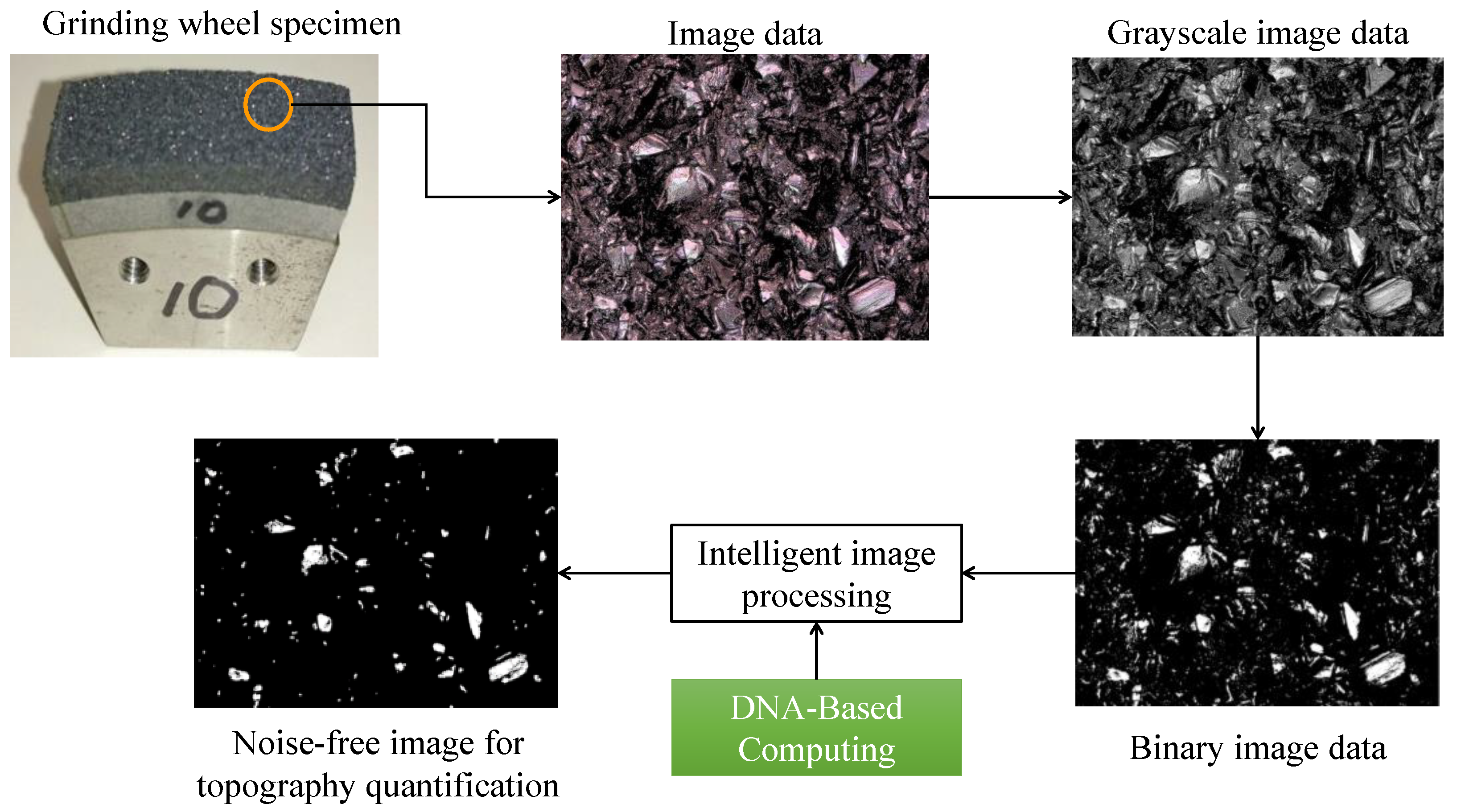
Figure 12.
DBC-driven intelligent image processing for grinding wheel surface topography quantification.
Figure 12.
DBC-driven intelligent image processing for grinding wheel surface topography quantification.

Table 1.
Grinding wheel and other specifications.
| Grinding Wheel | Vitrified CBN Grinding Wheel (BN140M100V) Diameter 140 mm, Width 10 mm |
|---|---|
| Grinding wheel rotational speed (N) | 5000 rpm (min−1) |
| Dresser | Prismatic diamond rotary dresser Diameter 50 mm, angle 0.2 mm 120 prismatic diamond grids in the circumferential direction |
| Dresser rotational speed (n) | 4200, 5600, 7000, 12,600, 15,400, and 19,600 rpm (min−1) |
| Velocity Ratio (VR) | ±0.3, ±0.5, ±0.9, ±1.1, and ±1.4 |
| Dressing depth of cut (ap) | 2.0 µm per pass for 15 times (total depth of cut: 30 µm) |
| Dressing feed rate (f) | 16.7 mm/s (0.2 mm/rev) |
| Coolant | WS90 |
Table 2.
Genetic codes [32].
Table 2.
Genetic codes [32].
| No | Amino Acids | Single-Letter Symbol of Amino Acids | Codons (In Terms of Three-Letter DNA Bases) |
|---|---|---|---|
| 1 | Isoleucine | I | ATT, ATC, ATA |
| 2 | Leucine | L | CTT, CTC, CTA, CTG, TTA, TTG |
| 3 | Valine | V | GTT, GTC, GTA, GTG |
| 4 | Phenylalanine | F | TTT, TTC |
| 5 | Methionine | M | ATG |
| 6 | Cysteine | C | TGT, TGC |
| 7 | Alanine | A | GCT, GCC, GCA, GCG |
| 8 | Glycine | G | GGT, GGC, GGA, GGG |
| 9 | Proline | P | CCT, CCC, CCA, CCG |
| 10 | Threonine | T | ACT, ACC, ACA, ACG |
| 11 | Serine | S | TCT, TCC, TCA, TCG, AGT, AGC |
| 12 | Tyrosine | Y | TAT, TAC |
| 13 | Tryptophan | W | TGG |
| 14 | Glutamine | Q | CAA, CAG |
| 15 | Asparagine | N | AAT, AAC |
| 16 | Histidine | H | CAT, CAC |
| 17 | Glutamic acid | E | GAA, GAG |
| 18 | Aspartic acid | D | GAT, GAC |
| 19 | Lysine | K | AAA, AAG |
| 20 | Arginine | R | CGT, CGC, CGA, CGG, AGA, AGG |
| 21 | None (stop) | X # | TAA, TAG, TGA |
# Generally, the symbol “*” is used to represent stop codons. Since “*” might be confused with other symbols, the letter X is chosen here to represent the stop codons.
Table 3.
Translation rules.
| Protk,l | Rk,l |
|---|---|
| I | ATT, ATC, or ATA |
| L | CTT, CTC, CTA, CTG, TTA, or TTG |
| V | GTT, GTC, GTA, or GTG |
| F | TTT or TTC |
| M | ATG |
| C | TGT or TGC |
| A | GCT, GCC, GCA, or GCG |
| G | GGT, GGC, GGA, or GGG |
| P | CCT, CCC, CCA, or CCG |
| T | ACT, ACC, ACA, or ACG |
| S | TCT, TCC, TCA, TCG, AGT, or AGC |
| Y | TAT or TAC |
| W | TGG |
| Q | CAA or CAG |
| N | AAT or AAC |
| H | CAT or CAC |
| E | GAA or GAG |
| D | GAT or GAC |
| K | AAA or AAG |
| R | CGT, CGC, CGA, CGG, AGA, or AGG |
| X | TAA, TAG, or TGA |
Publisher’s Note: MDPI stays neutral with regard to jurisdictional claims in published maps and institutional affiliations. |
© 2021 by the authors. Licensee MDPI, Basel, Switzerland. This article is an open access article distributed under the terms and conditions of the Creative Commons Attribution (CC BY) license (https://creativecommons.org/licenses/by/4.0/).
Share and Cite
MDPI and ACS Style
Kubo, A.; Teti, R.; Ullah, A.S.; Iwadate, K.; Segreto, T. Determining Surface Topography of a Dressed Grinding Wheel Using Bio-Inspired DNA-Based Computing. Materials 2021, 14, 1899. https://doi.org/10.3390/ma14081899
AMA Style
Kubo A, Teti R, Ullah AS, Iwadate K, Segreto T. Determining Surface Topography of a Dressed Grinding Wheel Using Bio-Inspired DNA-Based Computing. Materials. 2021; 14(8):1899. https://doi.org/10.3390/ma14081899
Chicago/Turabian StyleKubo, Akihiko, Roberto Teti, AMM Sharif Ullah, Kenji Iwadate, and Tiziana Segreto. 2021. "Determining Surface Topography of a Dressed Grinding Wheel Using Bio-Inspired DNA-Based Computing" Materials 14, no. 8: 1899. https://doi.org/10.3390/ma14081899
Note that from the first issue of 2016, this journal uses article numbers instead of page numbers. See further details here.