Article

Morphological Characterization and Effective Thermal Conductivity of Dual-Scale Reticulated Porous Structures

1
Department of Mechanical and Process Engineering, ETH Zürich, Sonneggstrasse 3, 8092 Zürich, Switzerland
2
Solar Technology Laboratory, Paul Scherrer Institute, 5232 Villigen PSI, Switzerland
*
Author to whom correspondence should be addressed.
Materials 2014, 7(11), 7173-7195; https://doi.org/10.3390/ma7117173
Submission received: 3 September 2014 / Revised: 13 October 2014 / Accepted: 15 October 2014 / Published: 28 October 2014
(This article belongs to the Section Porous Materials)

Abstract

:
Reticulated porous ceramic (RPC) made of ceria are promising structures used in solar thermochemical redox cycles for splitting CO2 and H2O. They feature dual-scale porosity with mm-size pores for effective radiative heat transfer during reduction and µm-size pores within its struts for enhanced kinetics during oxidation. In this work, the detailed 3D digital representation of the complex dual-scale RPC is obtained using synchrotron submicrometer tomography and X-ray microtomography. Total and open porosity, pore size distribution, mean pore diameter, and specific surface area are extracted from the computer tomography (CT) scans. The 3D digital geometry is then applied in direct pore level simulations (DPLS) of Fourier’s law within the solid and the fluid phases for the accurate determination of the effective thermal conductivity at each porosity scale and combined, and for fluid-to-solid thermal conductivity from 10−5 to 1. Results are compared to predictions by analytical models for structures with a wide range of porosities 0.09–0.9 in both the strut’s µm-scale and bulk’s mm-scale. The morphological properties and effective thermal conductivity determined in this work serve as an input to volume-averaged models for the design and optimization of solar chemical reactors.

1. Introduction

Foam-type reticulated porous ceramics (RPC) structures are applied in a broad range of physical processes requiring enhanced heat and mass transfer [1,2]. Applications include microelectronics cooling [3], soil dynamics [4,5], catalytic reactors [6], radiant burners [7], tissue engineering [3,8] and volumetric heat exchangers for the conversion of concentrated solar energy [9,10,11]. Of special interest of the latter application is the solar-driven thermochemical redox cycle for splitting CO2 and H2O [12,13,14,15,16], consisting of: (1) a high-temperature endothermic reduction, in which a metal oxide is thermally reduced and oxygen is evolved; and (2) a lower-temperature exothermic oxidation, in which the reduced oxide is re-oxidized with H2O and CO2 to form H2 and CO (syngas), and further processed to liquid hydrocarbon fuels. Ceria-based oxides have emerged as highly attractive redox materials because of the rapid oxygen transport in the bulk [14,15,16,17,18]. Various porous structures made of ceria have been investigated for enhanced reaction rates [18,19,20], including structures with submicron-sized interconnected pores, but these are problematic to retain because of partial sintering at elevated temperatures [19]. Furthermore, their high optical thickness inhibits penetration of concentrated solar radiation, resulting in non-uniform heating and temperature distributions [14]. Most recently, Furler et al. [15] presented a unique and morphologically stable RPC structure featuring dual-scale porosity: mm-size pores with struts containing micron-size pores. The mm-size pores enable volumetric absorption of concentrated solar radiation and effective heat transfer during the reduction step, while the micron-size pores within the struts offer increased specific surface area leading to enhanced reaction kinetics during the oxidation step.
Optimization of solar reactors for thermochemical redox cycles requires computational models of heat transfer and fluid dynamics coupled to the reaction kinetics [14,21]. Since resolving the solar reactor at the pore scale would require tremendous computational demand, volume-averaging theory is often applied for solving the mass, energy, and momentum conservation equations using effective heat and mass transport properties [22,23,24,25]. These can be determined accurately by direct pore-level simulations (DPLS) using the detailed 3D digital geometry of the structure obtained by computer tomography (CT) [26,27,28]. For example, the Monte Carlo ray-tracing method has been applied at the pore level for solving the radiative heat transfer equations and determining the effective extinction coefficient and scattering phase function [29], and the finite volume (FV) technique has been applied at the pore level for solving the Navier-Stokes equations and determining the effective thermal conductivity, permeability, and heat transfer coefficient [30,31].
In this work we apply the tomography-based methodology to investigate RPC structures made of ceria with dual-scale porosity in the mm and µm scales. This structure is schematically depicted in Figure 1 [15]. The total and open porosity, pore size distribution, mean pore diameter and specific surface area are extracted from the CT-scans. The effective thermal conductivity is determined by DPLS for the RPC with non-porous struts and for the RPC with dual-scale porosity. We investigate the effect that the dual-scale porosity has on the morphological properties and on the conduction heat transfer across the RPC, and further compare the results to predictions by analytical models for structures with a wide range of porosities in both the strut’s µm-scale and bulk’s mm-scale.
Figure 1. Ceria RPC with dual-scale porosity: mm-size pores for volumetric radiative absorption and effective heat transfer (a) during the reduction step, and struts containing micron-sized pores leading to increased specific surface area (b) for enhanced reaction kinetics during the oxidation step.
Materials 07 07173 g001

2. Experimental

2.1. RPC Synthesis

The dual-scale RPC structure is manufactured using the Schwartzwalder foam replication method [32]. An organic foam template is coated with multiple slurry layers containing ceria particles and micron-sized carbon grains [15]. The carbon pore former content ranges from 10 to 50 vol%. After firing at high temperatures (>1800 K), the bearing carbon foam and grains are burned und the desired foam-type structure undergoes sintering.

2.2. Synchrotron Submicrometer Tomography

Strut samples are scanned using synchrotron submicrometer tomography with a voxel (3D pixel) size of vs = 325 nm and a 0.832 × 0.832 × 0.702 mm3 field of view. The high-resolution CT is performed at the Swiss Light Source (SLS) of the Paul Scherrer Institute (PSI, Villigen, Switzerland) with the TOMCAT beamline for 40 keV photon energy, 400 µA beam current, a 100 µm thick aluminium filter, 40 µm thick copper filter, a 10 µm thick iron filter, 20× geometrical magnification, 1 s exposure time, 1001 projections. Figure 2 shows exemplary tomograms of strut samples manufactured with various concentrations of pore former ranging from 10 to 50 vol% and their corresponding 3D reconstructions of the pore space within isotropic strut regions. One tomogram contains 2560 × 2560 pixels. Numerous strut samples are scanned to verify reproducibility.
Figure 2. Synchrotron submicrometer computer tomograms of single RPC struts manufactured with various pore former concentrations (10, 20, 30, and 50 vol%) and their corresponding 3D digital reconstruction of the void space within isotropic porous strut region.
Materials 07 07173 g002

2.3. Micrometer Tomography

A ceria RPC sample with 10 pores per inch (ppi) is scanned by micrometer tomography with a voxel size of vs = 35.7 µm and a 36.56 × 36.56 × 36.56 mm3 field of view. The low-resolution CT is performed with an unfiltered polychromatic X-ray beam at the Swiss Federal Laboratories for Materials Science and Technology (EMPA, Dübedorf, Switzerland) for 150 keV photon energy, 45 µA beam current, 6.272 s exposure time and 721 projections. Figure 3 shows a tomogram and its corresponding 3D digital reconstruction of the scanned RPC sample. One tomogram contains 1024 × 1024 pixels.
Figure 3. Computer tomogram of the RPC with mm-sized pores and 3D rendering of a cropped cubic sample.
Materials 07 07173 g003

3. Morphological Characterization

3.1. Porosity

For the analysis of the strut structures, isotropic regions within submicrometer tomograms are cropped with the size of 501 × 501 × 501 voxels (0.163 × 0.163 × 0.163 mm3). For the analysis of the RPC structures, micrometer tomograms are cropped to 500 × 500 × 500 voxels (17.85 × 17.85 × 17.85 mm3). The cropped 8 bit tomograms obtained from measurements are pre-processed with a 3D Gaussian blurring filter to remove unwanted image noise derived from the photon sensor. Histograms computed from 3D tomogram stacks show bimodal character representing two grey scale pixel classes, with the threshold found by Otsu’s method of intra-class variance minimization [33,34]. Finally, based on the threshold, each pixel is assigned to be either void or solid. Porosity, ε = Vf/V, is defined as the ratio between the void space volume and the total cube volume. It is calculated by counting void and solid voxels of the 3D stack. The representative elementary volume (REV) defines the minimum volume containing a porous zone for which the continuum assumption is valid. It is determined from incrementally growing cubic subvolumes until their calculated porosities convergences within a certain band, ±γ. The conditions for the minimum edge length of the REV are [27]:
lREV = min{LL* |ε − γ < ε(VL*) < ε + γ},  γ << 1
where VL* is the sample subvolume and L* is the edge length of the sample subvolume. For the RPC with a porosity band of γ = 0.05, lREV ≥ 6.6 mm, which leads to cube structures larger than 186 voxels edge length. For the µm-sized struts with a porosity band of γ = 0.05, lREV ≥ 76.1 µm, which leads to cube structures larger than 235 voxels edge length.
Dual-scale porosity, εdual, is calculated from strut-scale porosity, εstrut, and RPC-scale porosity, εRPC, as:
εdual = εRPC + (1 − εRPC) ∙ εstrut
εstrut is linearly fitted to the pore former concentration, ϕ, as εstrut = 0.008707 ϕ. RPC structures with varying strut thicknesses are generated by altering the original segmented tomography scans through a dilation process with 3D spherical elements of a certain diameter, d, with Materials 07 07173 i001. Table 1 lists the dilation radius, digital porosity, and mean pore diameter of the original RPC reconstruction and of the digitally altered RPC for 3 increasing strut thicknesses, and the corresponding digital section cut and 3D rendering. As expected, porosity and mean pore diameter of the RPC decrease with increasing strut dilation because the thicker struts consume void space.
Of special interest is the connectivity of the µm-sized pores within the struts. The pore connectivity scales directly with the specific surface area reachable by reacting gases, and thus scales with the fuel production rates [15]. Open porosity, εopen, is defined as the pore space accessible from one of the 6 cube sample surfaces. An iterative routine starts searching from one cube side for connected neighbour void voxels in order to find all pores connected to this side. This reconstruction is performed to detect closed pores within the structure that account for the porosity but are not exposed to the gaseous reactants. Table 2 shows exemplary results of total and open porosity for strut samples with various pore former concentrations.
Table 1. Dilation radius, digital porosity, and mean pore diameter of the original RPC reconstruction and of the digitally altered RPC for increasing strut thickness, and the corresponding digital section cut and 3D rendering.
rdil (voxel)02510
rdil (mm)00.0710.1790.357
εRPC (–)0.8230.7560.6440.459
dmean (mm)2.322.211.981.64
Digital section cut through 3D structure at h = 50% Materials 07 07173 i002 Materials 07 07173 i003 Materials 07 07173 i004 Materials 07 07173 i005
3D rendering of RPC with mm-sized pores Materials 07 07173 i006 Materials 07 07173 i007 Materials 07 07173 i008 Materials 07 07173 i009
Table 2. Strut and open porosity, mean pore diameter, and the corresponding 3D rendering for strut samples manufactured with various pore former concentrations.
ϕ (vol%)10203050
εstrut (–)0.11950.17970.26050.4436
εopen (–)0.00950.01020.21670.4423
dmean (µm)9.2211.509.629.12
3D rendering of connected pore space Materials 07 07173 i010 Materials 07 07173 i011 Materials 07 07173 i012 Materials 07 07173 i013
Figure 4 shows all results of the porosities collected from selected 3D tomography reconstructions. εopen is presented with error bars because 6 evaluations are obtained per sample (one from each side). For ϕ ≤ 20 vol%, there is no pore connectivity observed as seen graphically in Table 2. For ϕ ≥ 30 vol%, the majority of the pores are connected and the pore network passes through the entire cube sample. For 50 vol%, practically every pore is connected to the pore network since the open porosity and total porosity are almost the same εopen ≈ εstrut. For high RPC porosity, e.g., εRPC = 0.825, the dual-scale porosity changes by less than 0.1 for ϕ = 50 vol% because only 17.5% of the volume is filled with µm-sized pores within the thin struts (see Figure 4). For lower RPC porosities, e.g., εRPC = 0.459, there is a stronger trend for increasing ϕ since there is more solid to be filled with µm-sized pores. The porosities of the model fit for ϕ = 0 vol% represent εRPC as listed in Table 1.
To investigate the transition from closed pores to interconnected pores in a systematic way, spheres with a small Gaussian size distribution of 2–3 voxels are randomly placed within the 3D volume. Pores of such artificially generated structures get connected between εstrut = 0.2 and 0.3. Such connectivity behavior is consistent with empirical correlations of the effective gas diffusivity within porous carbon [35]. Figure 4 also shows the comparison between the numerically determined εopen and the experimentally measured values by mercury intrusion porosimetry (MIP) [36,37], as reported by Furler et al. [15]. The agreement is reasonable well. For ϕ = 30 vol%, the experimentally measured εopen is lower than the numerically determined one due to poor pore connectivity across coating layers, as seen in Figure 5. This anisotropic region results from the 2-step coating applied during the fabrication process, and it is not considered in the determination of morphological properties and effective thermal conductivity within isotropic regions.
Figure 4. Total and open porosity as a function of the pore former concentration used to manufacture the µm-sized strut pores, total dual-scale porosity of RPC (original and digitally altered strut thickness).
Materials 07 07173 g004
Figure 5. Poor pore connectivity across fabrication layer originating from 2-step coating. (a) tomogram of a strut sample manufacture with 50 vol% carbon grain pore former. (b) 3D rendering of the void phase with pronounced solid barrier across the two coating layers.
Materials 07 07173 g005

3.2. Pore Size Distribution

Pore size distribution is determined by applying a morphology-altering algorithm to the digitally segmented 3D structure consisting of an inversion of the solid and void space, followed by erosion and dilation with successively increasing spherical elements of diameter d with Materials 07 07173 i001. In a last step, the algorithm inverts back the solid and void space. The cumulative pore size distribution 1 − F(d) is defined as the ratio of the opening-closing porosity, εoc(d), and the original porosity [27]:
Materials 07 07173 i014
The pore size distribution is then calculated as: f(d) = dF(d)/dd. Figure 6 shows the cumulative pore size distribution (left y-axis) and pore size distribution (right y-axis) as a function of df(d) agrees qualitatively well with the values obtained by mercury intrusion porosimetry measurements. The mean pore diameter is then defined in such a way to split the area under the pore size distribution curve into two equal areas [27].
Materials 07 07173 i015
The mean pore diameter for porous strut samples with various concentrations of pore former in the range 10–50 vol% is listed in Table 2. As expected, dmean remains independent of ϕ at around 10 µm because the same pore forming material is used to manufacture all samples.
Figure 6. Cumulative pore size distribution (left y-axis) and pore size distribution (right y-axis) obtained by morphology operations with spherical structuring elements of diameter d.
Materials 07 07173 g006

3.3. Specific Surface Area

The specific surface area (SSA) is determined in three different ways: (1) using statistical two-point correlation function computed on the 3D segmented structures with an in-house Fortran code; (2) resampling of the phase interface area with a surface mesh-based algorithm using the open source software ImageJ (version 1.47v, Java 1.6.0_20 (64-bit)) [38] extended with the free BoneJ plugin (version 1.3.11) [39]; and (3) using the actual phase interface area of tetrahedral 3D meshes generated with an in-house Fortran code [40]. The in-house mesh generator covers the void and solid domain with tetrahedral elements for unstructured body-fitted grids and subsequently refines the elements at the phase boundary. These 3D meshes are later used to solve the steady-state energy conservation equation to determine the effective thermal conductivity. The two point correlation s2(r) is a statistical function that indicates the probability of two arbitrary points Ψ(r) and Ψ(r + rŝ) separated by the distance r to be in the void phase [41]:
Materials 07 07173 i016
where Ω is the solid angle and V the cube volume. Porosity and specific surface area are then calculated using the following expressions [27,30]:
s2 (r = 0) = ε
s2 (r → ∞) = ε2
Materials 07 07173 i017
A code loops once through the entire structure (x-, y-, z-direction), counts each void voxel, and computes s2(r = 0) in a digitally exact manner. Additionally, the code counts for each void voxel the number of direct neighbour void voxels in all 6 directions (-x, x, -y, y, -z, z) and computes 6·s2(r = 1). The volumetric specific surface area is then calculated as:
Materials 07 07173 i018
The specific surface area is presented in two different units: per total volume (fluid+solid phases), A0 [m2 · m−3], and per ceria mass, ssa [m2 · g−1]. The density of ceria is ρCeO2 = 7.22 g/cm3 [21,42]. Dual-scale A0 is calculated by multiplying A0 determined for the struts by the solid volume fraction of the RPC: A0,dual = (1 − εRPC) · A0,strut. A0 of RPC with non-porous struts is converted to ssa by: ssaRPC = A0,RPC/[(1 − εRPC) · ρCeO2]. Table 3 lists ssa of RPC with non-porous struts obtained from the original tomography scans and digitally dilated struts.
Table 3. ssa of RPC with non-porous struts obtained from tomography scans and digitally dilated struts.
rdil (voxel)02510
rdil (mm)00.0710.1790.357
ssaRPC,2pc (m2·g−1)9.06 × 10−45.89 × 10−44.07 × 10−42.62 × 10−4
ssaRPC.mesh (m2·g−1)6.39 × 10−44.98 × 10−43.75 × 10−42.64 × 10−4
Because ssa is defined per unit mass, the strut ssa is necessarily equal to the ssa of the entire structure, including mm and µm sized pores. Thus, A0,strut is used to calculate ssa of porous struts and dual-scale porous structures:
Materials 07 07173 i019
A0 and ssa are plotted as a function of ϕ in Figure 7a,b, respectively. Of special interest is the open ssa, which is directly related to the surface area reachable by the reacting gases for conversion of CO2 and H2O to CO and H2. The open ssa is calculated for the struts without closed pores. Open A0 and ssa are presented with error bars (standard deviation) for the data evaluated. Surface areas calculated from two-point correlation and phase interface area of the 3D meshes (black and white symbols) lie within close proximity to one another, whereas those calculated using ImageJ (grey symbols) are higher. This is because the two-point correlation is based on a statistical model leading to smoothing effects and the 3D meshes actually contain a smoothing algorithm for the phase interface, whereas the resampled phase interface of ImageJ incorporates fine mesh surface irregularities. For ϕ ≤ 20 vol%, the open ssa is smaller than the total ssa because the majority of the pores are not connected. For ϕ = 30 vol% most pores are connected and the open ssa approaches the total ssa. For ϕ = 50 vol%, open and total ssa are nearly identical because at this point there are practically no closed pores (see Table 2). Trend lines are plotted defining the mean value of all different calculation methods for total (solid) and open (dashed) A0 and ssa.
Figure 7. Total and open specific surface area, ssa, as a function of the pore former concentration used to manufacture the µm-sized strut pores: (a) volumetric specific surface area of µm-sized strut pores; and (b) specific surface area per ceria mass of porous struts.
Materials 07 07173 g007

4. Heat Conduction Modelling

The governing steady-state heat conduction equations within the solid phase and the stagnant fluid phase are given by:
Solid phase:  ∇(ksTs) = 0
Fluid phase:  ∇(kfTf) = 0
where ks and kf are the thermal conductivity of the solid and fluid, respectively. The cubic domain is schematically shown in Figure 8. The boundary conditions are given in Equations (13)–(17). An inlet and outlet temperature is set (Thot > Tcold) to provide a steady heat flux through the two phases with length L. Lateral walls of the sample cube are adiabatic. Local thermal equilibrium is assumed at the phase interface. Heat flux across the interface is driven by the temperature gradient and the thermal conductivities in each phase at the interface.
Inlet temperature:   Ts(z = 0) = Tf(z = 0) = Thot
Outlet temperature:   Ts(z = L) = Tf(z = L) = Tcold
Adiabatic lateral walls:   n · Materials 07 07173 i020 = 0
Local thermal equilibrium at phase interface: Ts = Tf
Heat flux across phase interface:  n·ksTs = n·kfTf
Figure 8. Schematic of the steady state heat conduction simulation setup with hot inlet temperature, Thot, at z = 0 and cold outlet temperature, Tcold, at z = L.
Materials 07 07173 g008
The governing volume-averaged steady-state equation for effective heat conduction within the isotropic porous structure reduces to one equation [22,23]:
∇(keff∇〈T〉) = 0
The effective thermal conductivity is calculated using the 1D Fourier’s law and the heat flux determined by DPLS:
Materials 07 07173 i022
where keff is the effective thermal conductivity of the cubic porous structure, Materials 07 07173 i023 
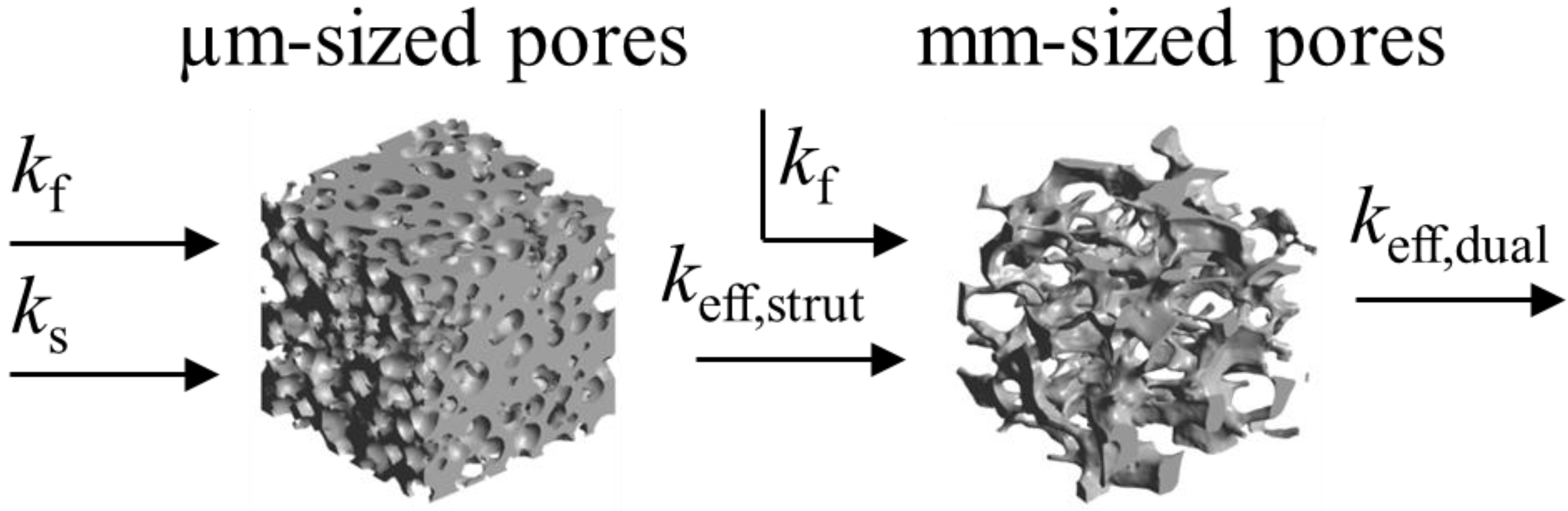
the effective heat flux at the inlet or outlet, and Aflux = L2 is the inlet or outlet area constraint with Thot or Tcold, respectively. The methodology for determination of keff for dual-scale porous structures is schematically shown in Figure 9. In a first step, keff of the strut with µm-sized pores (keff,strut) is determined according Equation (19). In a second step, this keff,strut serves as an input for the solid domain of a further simulation performed with the mm-sized pores of the RPC.
Figure 9. Methodology for the determination of the effective thermal conductivity of the RPC with dual-scale porosity.
Materials 07 07173 g009
Numerical DPLS are performed for RPC with non-porous/porous struts with/without digital strut dilation for different fluid-solid thermal conductivity ratios ranging from 10−5 up to 1. The cases covered include 4 RPC with non-porous struts (original scan and digitally dilated struts with 2, 5, and 10 voxels) and 16 RPC with porous struts (i.e., 4 RPC, each with 4 different strut porosities ϕ = 10, 20, 30, 50 vol%). Simulations are performed using a commercial computational fluid dynamics (CFD) software (ANSYS® Academic Research, release 14.0). Initially, grid resolution study is performed, indicating convergence for structures containing element sizes between 0.57 µm at fluid-solid interface to 2.28 µm within bulk for the µm-size pores within the struts, and between 62.0 µm at fluid-solid interface to 247.9 µm within bulk for the mm-size pores of the RPC. Typical number of elements is 20 million, yielding an error of less than 1% compared to the finest mesh tested of 40 million. The correctness of the DPLS was verified by solving simple geometrical cases with exact analytical solutions, while its accuracy was fine-tuned by grid refinement.
Figure 10 shows the ratio of the effective thermal conductivity to the solid thermal conductivity vs. the ratio of the fluid-to-solid thermal conductivity for a single porous strut (ϕ = 50 vol%), a RPC with non-porous struts, and a RPC with porous struts (ϕ = 50 vol% and 0 mm strut dilation). The analytical curves for serial and parallel slabs are indicating the maximum and minimum possible heat flux [43,44]. These exemplary simulation results correspond to εstrut = 0.410 and εRPC = 0.825, leading to εdual = 0.897. keff decreases with increasing porosity and decreasing kf/ks. For kf/ks < 10−3, keff does not significantly change anymore, indicating heat conduction dominated by the solid domain (e.g., for vacuum applications). In that range, the ratio of keff for RPC with non-porous struts to keff for RPC with porous struts is 2.4. As expected, this ratio approaches 1 for increasing kf/ks as the thermal conductivities of the fluid and solid phases approach each other. The serial and parallel heat conduction mode of the lumped fluid and solid material bracket the minimum and maximum possible heat flux (also called Wiener lower and upper bound), respectively [43,44]. As expected, the simulation results (black symbols) are between the minimum (white symbols with dashed line) and maximum (white symbols with solid line) possible heat flux for each porosity.
Table 4 lists various analytical models for keff [31,45]. For simplicity, analytical equations are given in terms of η = kf/ks, and ςeff = keff/ks. Several models allow fitting with geometrical shaping parameters. They were least-squares fitted to three different sets of simulation data: (1) keff,strut for a single porous strut (black squares shown in Figure 10); (2) keff,RPC for a RPC with non-porous struts (black circles shown in Figure 10); and (3) keff,dual for a RPC with porous struts (black triangles shown in Figure 10). To identify the model which agrees best with all data sets, an overall least-squares approximation, keff,all, was fitted for all simulation data.
Figure 10. Ratio of the effective thermal conductivity to the solid thermal conductivity vs. ratio of the fluid-to-solid thermal conductivity for a single porous strut (ϕ = 50 vol%), a RPC with non-porous struts, and a RPC with porous struts (ϕ = 50 vol%). The analytical curves for serial and parallel slabs are indicating the maximum and minimum possible heat flux.
Materials 07 07173 g010
Table 4. Analytical models for keff.
Model IDModelAnalytical Expression Materials 07 07173 i024Fitting Parameter
1Parallel slabs [43,44,46]ςeff = εη + (1 − ε)None
2Serial slabs [43,44,46] Materials 07 07173 i025None
3Hashin and Shtrikman upper bound [47] Materials 07 07173 i026None
4Hashin and Shtrikman lower bound [47] Materials 07 07173 i027None
5Woodside & Messmer [48] Materials 07 07173 i028None
6Russell [49] Materials 07 07173 i029None
7Loeb [50] Materials 07 07173 i030None
8Maxwell model [45,51,52,53] Materials 07 07173 i031None
9Schuetz-Glicksmann [54,55] Materials 07 07173 i032None
10Bhattacharya et al. [56] Materials 07 07173 i033r
χ = 2rν
Materials 07 07173 i034
Materials 07 07173 i035
Materials 07 07173 i036
Materials 07 07173 i037
Materials 07 07173 i038
11Boomsma and Poulikakos [57] Materials 07 07173 i039e
Materials 07 07173 i040
Materials 07 07173 i041
Materials 07 07173 i042
Materials 07 07173 i043
Materials 07 07173 i044
12Hamilton [58] Materials 07 07173 i045n
13Miller bound [59] Materials 07 07173 i046 Materials 07 07173 i047
Materials 07 07173 i048
14Calmidi and Mahajan [60]ςeff = εη + A(1 − ε)nA
n
15Dul’nev and Zarichnyak [22,30,61,62] Materials 07 07173 i050f
16Extended three-resistor model (this work)f = c0 + c1ε + c2ε2c0
Materials 07 07173 i050c1
c2
17Scalable three-resistor model (this work) Materials 07 07173 i052a
b
c
The root-mean-square error (RMS) is defined to compare keff calculated by the analytical models with that determined by our simulation:
Materials 07 07173 i053
where n is the number of data points per data set over the entire range of keff/ks and kf/ks indicated in Figure 10. Table 5 lists the RMS for the three different simulation data sets and for keff,all. Only those models giving an RMS < 5% are considered appropriate. Models 1 to 9, which are not using any geometrical shaping parameter, give RMS > 10%. However, some models perform comparatively well for the prediction of keff,strut with a RMS < 5%: Hashin and Shtrikman upper bound [47] (3.0%), Russell [49] (4.8%), Loeb [50] (2.6%) and Maxwell [51] (3.0%) which is consistent with the findings by Petrasch et al. [31] for SiC foams. Serial slab and Hashin and Shtrikman lower bound give very inaccurate predictions of keff (RMS > 200%). This is because the serial bound model assumes no direct connection of solid paths between heat inlet and outlet area, which is obviously not the case for connected, but tortuous strut paths. The Schuetz-Glicksmann model [54,55] yields inaccurate results (21.6%) and predicts values out of the range of the Wiener lower and upper bounds for kf/ks > 0.33. The fitted model of Bhattacharya et al. [56] can accurately predict keff,strut (1.5%). However, for the other simulation data sets, RMS > 10%. The model of Boomsma and Poulikakos [57] cannot be applied. Model is not suitable because equations lead to negative length scales in section B (one of four resistances) for any porosity and fitting parameter combination, geometrically describing a non-physical difference between the half node side length and the ligament radius. The fitted model of Hamilton et al. [58] gives only keff,strut with RMS < 5%. The fitted Miller’s bound [59] model, shown in Figure 11a, accurately represents the simulation results for keff,strut (0.4%), keff,RPC (1.8%), keff,dual (2.1%) and keff,all (1.9%). This model assumes statistical bound for two-phase media and uses two fitting parameters, G1 and G2, including spherical (number Materials 07 07173 i054) up to platelike (number Materials 07 07173 i055) void and solid shapes. Miller’s bound model is restricted within the upper and lower bound of Hashin and Shtrikman [59] for all fitting parameters. The empirical model of Calmidi and Mahajan [60], shown in Figure 11b, is capable of predicting all three data sets and an overall data sets with a RMS < 5%. The model of Dul’nev and Zarichnyak [62] gives only keff,strut with a RMS < 5%. Dul’nev and Zarichnyak [22,30,61,62] propose a model using a linear combination of the Wiener lower and upper bounds with empirical fitting parameter, f, for weighting linear combination which is also called three-resistor model. However, if keff is fitted individually for each structure (porosity), an inverse trend of f is observed with porosity. Therefore, the three-resistor model is then extended by describing f as a 2nd-order polynomial function with porosity. Such extended three-resistor model, shown in Figure 11c, predicts keff,strut with RMS = 0.3% instead of 3.9%, keff,RPC with RMS = 1.6% instead of 9.2%, keff,dual with RMS = 2.2% instead of 9.8%, and keff,all with RMS = 2.3% instead of 12.6%. The three fitting parameters describing f with a 2nd-order polynomial function (c0, c1, c2) are replaced to allow the serial and parallel resistance, as well as their combination, to linearly scale with porosity, as shown schematically in Figure 12. Least-squares fitting of this modified three-resistor model, shown in Figure 11d, delivers the most accurate predictions: keff,strut with RMS = 0.1%, keff,RPC with RMS = 1.1%, keff,dual with RMS = 1.4%, and keff,all with RMS = 1.3%. The modified three-resistor model shows the best performance in prediction of keff with overall RMS < 1.5%. Fitting parameter a and b allow the lumped fluid and solid parts to deviate from actual ε within the parallel and serial slabs, respectively. Fitting parameter c allows linear combination of the serial and parallel slab to deviate from ε. This gives some degree of freedom for capturing different tortuous regions for a high porosity range (0.09 < ε < 0.9) and predicts the effective thermal conductivity more accurately compared to linear (or non-linear) combination of parallel/serial bounds and to Miller’s bound model.
Table 5. Root-mean-square (RMS) error of analytical models compared to three simulation data sets and to all simulation data.
ModelRMSkeff,strut (n = 24)keff,RPC (n = 24)keff,dual (n = 96)keff,all (n = 144)
1RMS (%)7.51626.86132.15828.620
2RMS (%)233.780223.485213.144218.449
3RMS (%)3.01016.56120.99218.466
4RMS (%)204.379207.200200.080202.003
5RMS (%)63.012139.992148.175136.255
6RMS (%)4.77217.82822.02419.497
7RMS (%)2.61115.24119.91617.443
8RMS (%)3.01016.56120.99218.466
9RMS (%)7.51626.86132.15821.621
10r0.29120.19720.12540.2684
RMS (%)1.48410.7385.82913.102
11RMS (%)N/A 1N/A 1N/A 1N/A 1
12n2.19851.63431.53251.5701
RMS (%)1.2475.8226.9846.868
13G11/90.12620.12680.1267
G20.14301/91/91/9
RMS (%)0.4091.8282.0711.880
14A1.02851.04821.07091.0360
n1.60831.59901.60951.5893
RMS (%)2.2174.7214.9334.571
15f0.83770.49540.42170.4865
RMS (%)3.9459.1649.75412.595
16c00.99720.33360.25810.9284
c1−0.46341.65701.6780−0.1850
c2−0.5544−1.9954−1.8817−0.6186
RMS (%)0.2611.6112.2022.294
17a1.31941.08231.05411.0548
b0.31810.64750.70080.7015
c0.20000.54440.62290.6223
RMS (%)0.1351.0571.3731.347
1 Model is not suitable because equations lead to negative length scales in section B (one of four resistances) for any porosity and fitting parameter combination, geometrically describing a non-physical difference between the half node side length and the ligament radius.
Figure 11. Ratio of the effective thermal conductivity to the solid thermal conductivity vs. ratio of the fluid-to-solid thermal conductivity, obtained by our simulation and by least-squares fitted models for structures with a high range of porosities (0.09 < ε < 0.9). Shown are: (a) Miller bound model [59]; (b) Calmidi and Mahajan model [60]; (c) extended three-resistor model; and (d) modified three-resistor model. The modified three-resistor model predicts keff with the lowest RMS.
Materials 07 07173 g011
Figure 12. (a) Common three-resistor model [22]; (b) modified three-resistor model with scaling parameter for the serial and parallel slab and their combination.
Materials 07 07173 g012

5. Summary and Conclusions

High and low resolution computer tomographic scans were performed on complex reticulated porous ceramics (RPC) structures to capture the 3D digital representations of their dual-scale porosity in the mm and µm range. The CT scans were processed with a Gaussian blurring filter for a clustering-based image thresholding of the void and solid phases using Otsu’s method. The struts containing µm-size pores were digitally dilated with spherical structuring elements generating structures with different thickness and porosity. The morphological properties analyzed include porosity, pore size distribution, specific surface area, and pore connectivity within representative sample volumes of the isotropic strut regions and of the RPC. The total strut porosity was linearly dependent on the concentration of pore forming agent, and no pore connectivity was observed for concentration less than 20 vol%, consistent with mercury intrusion porosimetry measurements. A well-connected pore network results in high specific surface area and penetration of reactant gas for high fuel production. The effective thermal conductivities of a single porous strut, a RPC with non-porous struts, and a RPC with porous struts (dual scale) were determined by direct pore level simulations of the heat conduction equation with a CFD code. Values were compared to predictions by analytical models over a wide range of porosities. Models without shaping parameters were generally inaccurate (overall RMS > 10%). Miller’s model with two shaping parameters predicted keff with RMS error below 2.1% and the modified three-resistor model with three empirical fitting parameters predicted keff with a RMS error below 1.5%. These analytical correlations are applicable to RPC with porosities in both the strut’s µm-scale and bulk’s mm-scale ranging from 0.09 to 0.9.
The morphological properties and effective thermal conductivity determined in this work serve as an input to volume-averaged models for the design and optimization of solar chemical reactors.

Acknowledgments

We gratefully acknowledge the financial support by the Swiss Competence Center Energy & Mobility, the Helmholtz–Gemeinschaft Deutscher Forschungszentren (Virtuelles Institut SolarSyngas), and the European Research Council under the European Union’s ERC Advanced Grant (SUNFUELS—No. 320541).

Nomenclature

A0,(.)
Volumetric specific surface area (m−1)
Aflux
Cross sectional inlet/outlet area of cubic sample for heat flux (m2)
ssa(.)
Physical specific surface area (Index: strut, RPC, dual) (m2 g−1)
d
Diameter of spherical structuring elements (m)
dmean
Mean pore diameter (m)
f(d)
Pore size distribution (–)
F(d)
Cumulative pore size distribution (–)
ks
Solid thermal conductivity (W m−1 K−1)
kf
Fluid thermal conductivity (W m−1 K−1)
keff,(.)
Effective thermal conductivity of porous structure (W m−1 K−1)
lREV
Cube edge length of representative elementary volume (m)
L
Cube edge length (m)
n
Number of simulation data points (–)
Materials 07 07173 i056
Heat flux through sample (W m−2 )
s2(r)
Two point correlation function (–)
Tcold
Cold side temperature (K)
Tf
Fluid temperature (K)
Thot
Hot side temperature (K)
Ts
Solid temperature (K)
vs
Voxel size (m)
V
Total sample cube volume (m3)
Vf
Void volume (m3)
ε(.)
Porosity (–)
γ
Error band of porosity (–)
ςeff
Ratio of effective to solid thermal conductivity (–)
η
Ratio of fluid to solid thermal conductivity (–)
ϕ
Pore former concentration (vol%)

Subscripts

2pc
2-point correlation
mesh
3D-mesh generated from digitally segmented structures
ImageJ
Calculated using open source software ImageJ
strut
Morphological property of porous strut
RPC
Morphological property of RPC with non-porous struts
dual
Morphological property of RPC with porous struts (dual-scale)
open
Open morphological property excluding closed pores
oc
Morphological property after applying opening-closing algorithm

Conflicts of Interest

The authors declare no conflict of interest.

References

  1. Bear, J.; Buchlin, J.M. Modelling and Applications of Transport Phenomena in Porous Media; Kluwer Academic Publishers: Dordrecht, The Netherlands, 1991; p. 380. [Google Scholar]
  2. Ho, C.K.; Webb, S.W. Gas Transport in Porous Media; Springer: Dordrecht, The Netherlands, 2006; p. 44. [Google Scholar]
  3. Vadász, P.T. Emerging Topics in Heat and Mass Transfer in Porous Media: From Bioengineering and Microelectronics to Nanotechnology; Springer: Dordrecht, The Netherlands, 2008; p. 328. [Google Scholar]
  4. Verruijt, A. An Introduction to Soil Dynamics; Springer: Dordrecht, The Netherlands, 2010; p. 433. [Google Scholar]
  5. Bear, J.; Verruijt, A. Modeling Groundwater Flow and Pollution: With Computer Programs for Sample Cases; D. Reidel Pub. Co.: Dordrecht, The Netherlands, 1987; p. 414. [Google Scholar]
  6. Dhamrat, R.S.; Ellzey, J.L. Numerical and experimental study of the conversion of methane to hydrogen in a porous media reactor. Combust. Flame 2006, 144, 698–709. [Google Scholar] [CrossRef]
  7. Pantangi, V.K.; Mishra, S.C.; Muthukumar, P.; Reddy, R. Studies on porous radiant burners for lpg (liquefied petroleum gas) cooking applications. Energy 2011, 36, 6074–6080. [Google Scholar] [CrossRef]
  8. Zermatten, E.; Vetsch, J.R.; Ruffoni, D.; Hofmann, S.; Müller, R.; Steinfeld, A. Micro-computed tomography based computational fluid dynamics for the determination of shear stresses in scaffolds within a perfusion bioreactor. Ann. Biomed. Eng. 2014, 42, 1085–1094. [Google Scholar] [CrossRef]
  9. Fend, T.; Hoffschmidt, B.; Pitz-Paal, R.; Reutter, O.; Rietbrock, P. Porous materials as open volumetric solar receivers: Experimental determination of thermophysical and heat transfer properties. Energy 2004, 29, 823–833. [Google Scholar] [CrossRef]
  10. Hischier, I.; Leumann, P.; Steinfeld, A. Experimental and numerical analyses of a pressurized air receiver for solar-driven gas turbines. J. Sol. Energy Eng. 2012, 134, 1–8. [Google Scholar]
  11. Hischier, I.; Poživil, P.; Steinfeld, A. A modular ceramic cavity-receiver for high-temperature high-concentration solar applications. J. Sol. Energy Eng. 2011, 134. [Google Scholar] [CrossRef]
  12. Romero, M.; Steinfeld, A. Concentrating solar thermal power and thermochemical fuels. Energy Environ. Sci. 2012, 5, 9234–9245. [Google Scholar] [CrossRef]
  13. Miller, J.E.; McDaniel, A.H.; Allendorf, M.D. Considerations in the design of materials for solar-driven fuel production using metal-oxide thermochemical cycles. Adv. Energy Mater. 2014, 4. [Google Scholar] [CrossRef]
  14. Furler, P.; Scheffe, J.; Gorbar, M.; Moes, L.; Vogt, U.; Steinfeld, A. Solar thermochemical CO2 splitting utilizing a reticulated porous ceria redox system. Energy Fuels 2012, 26, 7051–7059. [Google Scholar]
  15. Furler, P.; Scheffe, J.; Marxer, D.; Gorbar, M.; Bonk, A.; Vogt, U.; Steinfeld, A. Thermochemical CO2 splitting via redox cycling of ceria reticulated foam structures with dual-scale porosities. PCCP 2014, 16, 10503–10511. [Google Scholar] [CrossRef]
  16. Furler, P.; Scheffe, J.R.; Steinfeld, A. Syngas production by simultaneous splitting of H2O and CO2 via ceria redox reactions in a high-temperature solar reactor. Energy Environ. Sci. 2012, 5, 6098–6103. [Google Scholar] [CrossRef]
  17. Ackermann, S.; Scheffe, J.R.; Steinfeld, A. Diffusion of oxygen in ceria at elevated temperatures and its application to H2O/CO2 splitting thermochemical redox cycles. J. Phys. Chem. C 2014, 118, 5216–5225. [Google Scholar] [CrossRef]
  18. Chueh, W.C.; Falter, C.; Abbott, M.; Scipio, D.; Furler, P.; Haile, S.M.; Steinfeld, A. High-flux solar-driven thermochemical dissociation of CO2 and H2O using nonstoichiometric ceria. Science 2010, 330, 1797–1801. [Google Scholar] [CrossRef]
  19. Venstrom, L.J.; Petkovich, N.; Rudisill, S.; Stein, A.; Davidson, J.H. The effects of morphology on the oxidation of ceria by water and carbon dioxide. J. Sol. Energy Eng. 2012, 134. [Google Scholar] [CrossRef]
  20. Gibbons, W.T.; Venstrom, L.J.; de Smith, R.M.; Davidson, J.H.; Jackson, G.S. Ceria-based electrospun fibers for renewable fuel production via two-step thermal redox cycles for carbon dioxide splitting. Phys. Chem. Chem. Phys. 2014, 16, 14271–14280. [Google Scholar] [CrossRef]
  21. Keene, D.J.; Davidson, J.H.; Lipiński, W. A model of transient heat and mass transfer in a heterogeneous medium of ceria undergoing nonstoichiometric reduction. J. Heat Transfer 2013, 135. [Google Scholar] [CrossRef]
  22. Kaviany, M. Principles of Heat Transfer in Porous Media, 2nd ed.; Springer-Verlag: New York, NY, USA, 1995; p. 708. [Google Scholar]
  23. Whitaker, S. The Method of Volume Averaging; Series: Theory and Applications of Transport in Porous Media); Kluwer Academic: Dordrecht, The Netherlands, 1999; p. 219. [Google Scholar]
  24. Bodla, K.K.; Weibel, J.A.; Garimella, S.V. Advances in fluid and thermal transport property analysis and design of sintered porous wick microstructures. J. Heat Transf. 2013, 135. [Google Scholar] [CrossRef]
  25. Krishnan, S.; Murthy, J.Y.; Garimella, S.V. Direct simulation of transport in open-cell metal foam. J. Heat Transf. 2006, 128, 793–799. [Google Scholar] [CrossRef]
  26. Petrasch, J.; Meier, F.; Friess, H.; Steinfeld, A. Tomography based determination of permeability, dupuit-forchheimer coefficient, and interfacial heat transfer coefficient in reticulate porous ceramics. 2008, 29, 315–326. [Google Scholar]
  27. Petrasch, J.; Wyss, P.; Stämpfli, R.; Steinfeld, A. Tomography-based multiscale analyses of the 3D geometrical morphology of reticulated porous ceramics. J. Am. Ceram. Soc. 2008, 91, 2659–2665. [Google Scholar] [CrossRef]
  28. Bodla, K.K.; Murthy, J.Y.; Garimella, S.V. Microtomography-based simulation of transport through open-cell metal foams. Numer. Heat Transf. A Appl. 2010, 58, 527–544. [Google Scholar] [CrossRef]
  29. Petrasch, J.; Wyss, P.; Steinfeld, A. Tomography-based monte carlo determination of radiative properties of reticulate porous ceramics. J. Quant. Spectrosc. Radiat. Transf. 2007, 105, 180–197. [Google Scholar] [CrossRef]
  30. Haussener, S.; Coray, P.; Lipinski, W.; Wyss, P.; Steinfeld, A. Tomography-based heat and mass transfer characterization of reticulate porous ceramics for high-temperature processing. J. Heat Transf. 2010, 132. [Google Scholar] [CrossRef]
  31. Petrasch, J.; Schrader, B.; Wyss, P.; Steinfeld, A. Tomography-based determination of the effective thermal conductivity of fluid-saturated reticulate porous ceramics. ASME J. Heat Transf. 2008, 130. [Google Scholar] [CrossRef]
  32. Karl, S.; Somers, A.V. Method of Making Porous Ceramic Articles. U.S. Patent 3090094 A, 21 May 1963. [Google Scholar]
  33. Otsu, N. A threshold selection method from gray-level histograms. IEEE Trans. Syst. Man Cybern. 1979, 9, 62–66. [Google Scholar] [CrossRef]
  34. Sezgin, M.; Sankur, B.L. Survey over image thresholding techniques and quantitative performance evaluation. ELECTIM 2004, 13, 146–168. [Google Scholar]
  35. Zamel, N.; Li, X.; Shen, J. Correlation for the effective gas diffusion coefficient in carbon paper diffusion media. Energy Fuels 2009, 23, 6070–6078. [Google Scholar] [CrossRef]
  36. Giesche, H. Mercury porosimetry: A general (practical) overview. Part. Part. Syst. Charact. 2006, 23, 9–19. [Google Scholar] [CrossRef]
  37. Webb, P.A. An Introduction to the Physical Characterization of Materials by Mercury Intrusion Porosimetry with Emphasis on Reduction and Presentation of Experimental Data; Micromeritics Instrument Corp.: Norcross, GA, USA, 2001. [Google Scholar]
  38. Abràmoff, M.D.; Magalhães, P.J.; Ram, S.J. Image processing with imageJ. Biophoton. Int. 2004, 11, 36–43. [Google Scholar]
  39. Doube, M.; Kłosowski, M.M.; Arganda-Carreras, I.; Cordelières, F.P.; Dougherty, R.P.; Jackson, J.S.; Schmid, B.; Hutchinson, J.R.; Shefelbine, S.J. Bonej: Free and extensible bone image analysis in imageJ. Bone 2010, 47, 1076–1079. [Google Scholar] [CrossRef]
  40. Friess, H.; Haussener, S.; Steinfeld, A.; Petrasch, J. Tetrahedral mesh generation based on space indicator functions. Int. J. Numer. Methods Eng. 2013, 93, 1040–1056. [Google Scholar] [CrossRef]
  41. Berryman, J.G.; Blair, S.C. Use of digital image analysis to estimate fluid permeability of porous materials: Application of two-point correlation functions. J. Appl. Phys. 1986, 60, 1930–1938. [Google Scholar] [CrossRef]
  42. Mogensen, M.; Sammes, N.M.; Tompsett, G.A. Physical, chemical and electrochemical properties of pure and doped ceria. Solid State Ion. 2000, 129, 63–94. [Google Scholar] [CrossRef]
  43. Bruggeman, D.A.G. Berechnung verschiedener physikalischer konstanten von heterogenen substanzen. I. Dielektrizitätskonstanten und leitfähigkeiten der mischkörper aus isotropen substanzen. Ann. Phys. 1935, 416, 636–664. (In German) [Google Scholar] [CrossRef]
  44. Deissler, R.G.; Boegli, J.S. An investigation of effective thermal conductivities of powders in various gases. Trans. ASME 1958, 80, 1417–1425. [Google Scholar]
  45. Wang, M.; Pan, N. Predictions of effective physical properties of complex multiphase materials. Mater. Sci. Eng. R Rep. 2008, 63, 1–30. [Google Scholar] [CrossRef]
  46. DeVera, A.L.; Strieder, W. Upper and lower bounds on the thermal conductivity of a random, two-phase material. J. Phys. Chem. 1977, 81, 1783–1790. [Google Scholar] [CrossRef]
  47. Hashin, Z.; Shtrikman, S. A variational approach to the theory of the effective magnetic permeability of multiphase materials. J. Appl. Phys. 1962, 33, 3125–3131. [Google Scholar] [CrossRef]
  48. Woodside, W.; Messmer, J.H. Thermal conductivity of porous media. II. Consolidated rocks. J. Appl. Phys. 1961, 32, 1699–1706. [Google Scholar] [CrossRef]
  49. Russell, H.W. Principles of heat flow in porous insulators. J. Am. Ceram. Soc. 1935, 18, 1–5. [Google Scholar] [CrossRef]
  50. Loeb, A.L. Thermal conductivity: VIII, a theory of thermal conductivity of porous materials. J. Am. Ceram. Soc. 1954, 37, 96–99. [Google Scholar] [CrossRef]
  51. Maxwell, J.C. A Treatise on Electricity and Magnetism, 3rd ed.; Dover Publications: New York, NY, USA, 1954. [Google Scholar]
  52. Choy, T.C. Effective Medium Theory: Principles and Applications; Oxford University Press: Oxford, UK, 1999; p. 182. [Google Scholar]
  53. Sattler, K.D. Handbook of Nanophysics. Nanoparticles and Quantum Dots; Taylor & Francis: Boca Raton, FL, USA, 2011. [Google Scholar]
  54. Kamiuto, K. Modeling of composite heat transfer in open-cellular porous materials at high temperatures. In Cellular and Porous Material Thermal Properties Simulation Prediction; Wiley-VCH: Weinheim, Germany, 2008; pp. 165–198. [Google Scholar]
  55. Coquard, R.; Loretz, M.; Baillis, D. Conductive heat transfer in metallic/ceramic open-cell foams. Adv. Eng. Mater. 2008, 10, 323–337. [Google Scholar] [CrossRef]
  56. Bhattacharya, A.; Calmidi, V.V.; Mahajan, R.L. An analytical-experimental study for the determination of the effective thermal conductivity of high porosity fibrous foams. ASME Appl. Mech. Divis. Pupl. AMD 1999, 233, 13–20. [Google Scholar]
  57. Boomsma, K.; Poulikakos, D. On the effective thermal conductivity of a three-dimensionally structured fluid-saturated metal foam. Int. J. Heat Mass Transf. 2001, 44, 827–836. [Google Scholar] [CrossRef]
  58. Hamilton, R.L.; Crosser, O.K. Thermal conductivity of heterogeneous two-component systems. Ind. Eng. Chem. Fundam. 1962, 1, 187–191. [Google Scholar] [CrossRef]
  59. Miller, M.N. Bounds for effective electrical, thermal, and magnetic properties of heterogeneous materials. J. Math. Phys. 1969, 10, 1988–2004. [Google Scholar] [CrossRef]
  60. Calmidi, V.V.; Mahajan, R.L. The effective thermal conductivity of high porosity fibrous metal foams. J. Heat Transf. 1999, 121, 466–471. [Google Scholar] [CrossRef]
  61. Matsushita, M.; Monde, M.; Mitsutake, Y. Predictive calculation of the effective thermal conductivity in a metal hydride packed bed. Int. J. Hydrog. Energy 2014, 39, 9718–9725. [Google Scholar] [CrossRef]
  62. Dul’Nev, G.N.; Zarichnyak, Y.P. A study of the generalized conductivity coefficients in heterogeneous systems. Heat Transf. Sov. Res. 1970, 2, 89–107. [Google Scholar]

