How to Study Thermal Applications of Open-Cell Metal Foam: Experiments and Computational Fluid Dynamics

Abstract

This paper reviews the available methods to study thermal applications with open-cell metal foam. Both experimental and numerical work are discussed. For experimental research, the focus of this review is on the repeatability of the results. This is a major concern, as most studies only report the dependence of thermal properties on porosity and a number of pores per linear inch (PPI-value). A different approach, which is studied in this paper, is to characterize the foam using micro tomography scans with small voxel sizes. The results of these scans are compared to correlations from the open literature. Large differences are observed. For the numerical work, the focus is on studies using computational fluid dynamics. A novel way of determining the closure terms is proposed in this work. This is done through a numerical foam model based on micro tomography scan data. With this foam model, the closure terms are determined numerically.

1. Introduction

1.1. Thermal Applications

Heat exchangers are essential components in a wide range of thermal management applications, e.g., in the transport, domestic and industrial sectors. These devices are crucial because they have an influence on safety, environmental quality and energy use. In such devices, air is often used as a working fluid [1], due to its omnipresence. The low thermal conductivity results in an air-side thermal resistance, which can be more than 80% of the total thermal resistance in heat exchangers working with air [2]. Consequently, reducing this air-side thermal resistance can result in substantial performance augmentation, leading to cost, space, material and energy savings. Prior research has led to considerable improvements by investigating the influence of fluid characteristics, flow arrangements, material selection and extending the heat transfer surface area (through fins) [3].

In forced convection, these heat transfer enhancement techniques aim to maximize the product of the heat transfer coefficient and the heat transfer surface area per unit volume, whilst minimizing the air-side pressure drop. This results in all kinds of fin designs, most of the time heavily dependent on the application. The current state of the art fin type, for a non-corrosive environment, is the interrupted fin design, like the louvered fin or slit fins [4]. Further possible improvements can be achieved through the implementation of vortex generators. When placed near the wake zones of the tube, vortex generators can yield a significant improvement to the heat transfer [5].

In natural convection, a similar optimization approach is used. In this case, the problem is even more complex, as the flow resistance will affect local temperatures and heat transfer coefficients. Furthermore, radiation will play a significant role [6]. Pin fins and all kinds of different forms of plain fins (especially the inverted trapezoidal fin) can induce more air flow over the heat sink in comparison to a plain rectangular fin [7]. Further possible improvements can be achieved by the orientation of the fins themselves. For example, a flared pin design can improve the heat transfer performance significantly, as proposed by CoolInnovations [8]. Another optimization is making the fins themselves more porous by perforating them [9].

A development that fits within this optimization process of “conventional” fins is the use of porous media. One example of a porous medium that can be used as a heat exchanger is a packed bed of spheres, which has a porosity of around 60% [10]. Another porous material that has already drawn a lot of attention is open-cell metal foam. In Figure 1, the nomenclature of open-cell foam is shown. The struts of the foam are interconnected in the nodes forming both cells and pores.

Figure 1. Nomenclature of cast open-cell metal foam.

Figure 1. Nomenclature of cast open-cell metal foam.

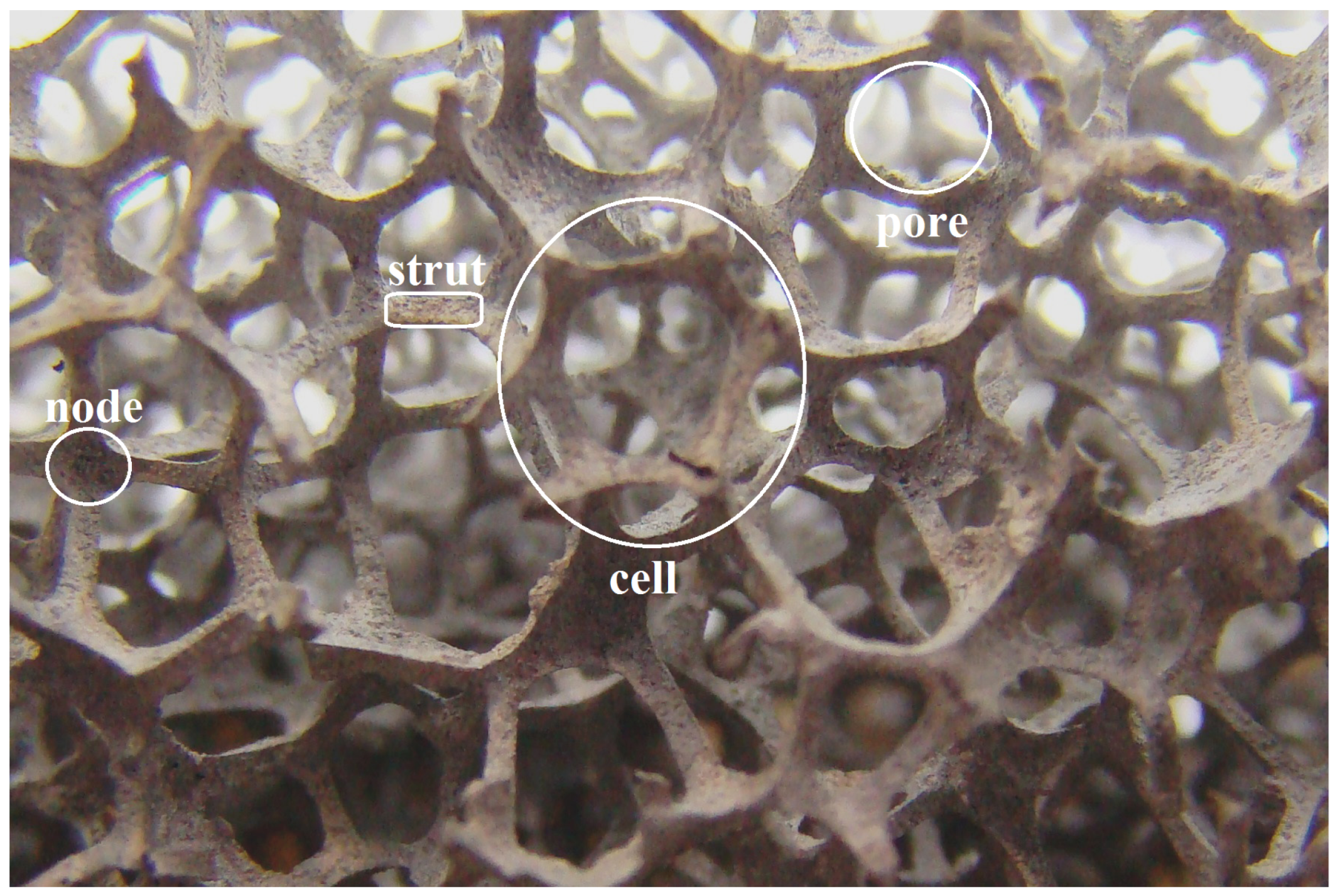
1.2. Open-Cell Metal Foam

There are different types of open-cell metal foam; this paper will focus on the foam type that performs best in thermal applications: cast open-cell metal foam, which has solid struts. Conversely, open-cell foam made through an electrophoretic deposition process has hollow struts. This significantly lowers its effective thermal conductivity up to one third of its cast alternative [11].

Cast foam originates from the late 1960s and was invented by the “Materials and Aerospace” division of Energy Research and Generation (ERG) [12]. This invention has led to the patent of Walz [13], which describes the manufacturing process of cast open-cell metal foam based on an organic preform. Most of the time, this preform consists of polyurethane. The metal foam by ERG Materials and Aerospace was intended for military and aerospace applications. Only since the mid 1990s, the technology became generally available for non-classified military and industrial applications. It is from that time that the annual publication rate on the topic has increased steadily (see Figure 2). The graph shows all conference and journal papers (excluding patents) with keywords “metal foam”, “heat transfer” and “open-cell” that were published each year in all journals indexed by Google Scholar. From 2000 on, the publication rate keeps increasing. This evolution has also triggered other manufacturers of cast open-cell metal foam to emerge. In 2000, the German company M-Pore GmbH, in Dresden [14] started making cast metal foam. Alveotec in France [15] and Constellium [16] in the Netherlands followed a few years later. Most of these companies are still closely related to the research industry. Constellium for example works together with The University of Sheffield, while Alveotec works closely together with the TEMISTh—research group in Marseille (France).

Figure 2. Evolution of the yearly number of publications since 1990 as indexed by Google Scholar using the following keywords: “metal foam”, “heat transfer” and “open-cell”.

Figure 2. Evolution of the yearly number of publications since 1990 as indexed by Google Scholar using the following keywords: “metal foam”, “heat transfer” and “open-cell”.

Open-cell cast metal foam manufactured by either ERG Materials and Aerospace or M-Pore is made with an investment casting process based on a polyurethane preform. As the fabrication process of the organic preform is influenced by gravity, the resulting cells are oval shaped (see Figure 3a). A deterministic approach to obtain a model of such an organic preform is based on minimizing the total film energy of the surface between the solid and fluid phase.

Figure 3. Two cast types of open-cell metal foam produced by (a) investment casting from a polyurethane perform and (b) leachable bed casting (example from Alveotec, painted black to increase emissivity).

Figure 3. Two cast types of open-cell metal foam produced by (a) investment casting from a polyurethane perform and (b) leachable bed casting (example from Alveotec, painted black to increase emissivity).

On the other hand, the metal foam by Alveotec and Constellium is made by casting metal over a stacked bed of soluble spheres. These spheres can be either salt spheres or sand with a polymer bonding agent [15]. After solidification of the metal, the spheres are then simply washed away with water. This process is known as leachable bed casting. The metal foam that is created with this manufacturing process has a more uniform and spherical cell shape (see Figure 3b).

Cast open-cell foam is known to have many interesting structural and functional properties:

• High porosity (higher than 80%). Typically, the porosity can go up to 95%. High porosity results in a low weight application.
• High interstitial surface area per unit volume.
• Good impact energy absorption [17].
• Excellent fluid mixing due to tortuous flow paths [18].
• Hybrid manufacturability: different foam materials (e.g., Al, Cu) can be sandwiched into one foam panel [19].
• Shapeable in three dimensions (obtainable via casting and/or co-casting techniques).
• Visually appealing.

A combination of these advantages results in metal foam already being in use in systems like the Porifera light-emitting diode (LED) system from TAL, Pittem, Belgium (Technical Architectural Lighting) and LED cooling for LOUPI Lighting in Pantin, France [20].

1.3. What Are the Thermal Cooling Applications with Open-Cell Foam?

The two effective ways to study thermal applications with open-cell metal foam are through experiments and/or with computational fluid dynamics (CFD) [1]. Of course, both tools have their upsides and downsides. Experiments have the advantage that, if they are performed correctly, they are reliable and can serve as proof to the industrial clients or as a reference for further academic research.

On the other hand, generally for thermal foam applications, a large number of parameters influence the thermal characterization of an application, amongst others:

• Type of open-cell metal foam: This includes the material and manufacturing technique, on the one hand, and the thickness of the foam, on the other hand. Both of these parameters will affect the effective solid conductivity and heat transferring surface area.
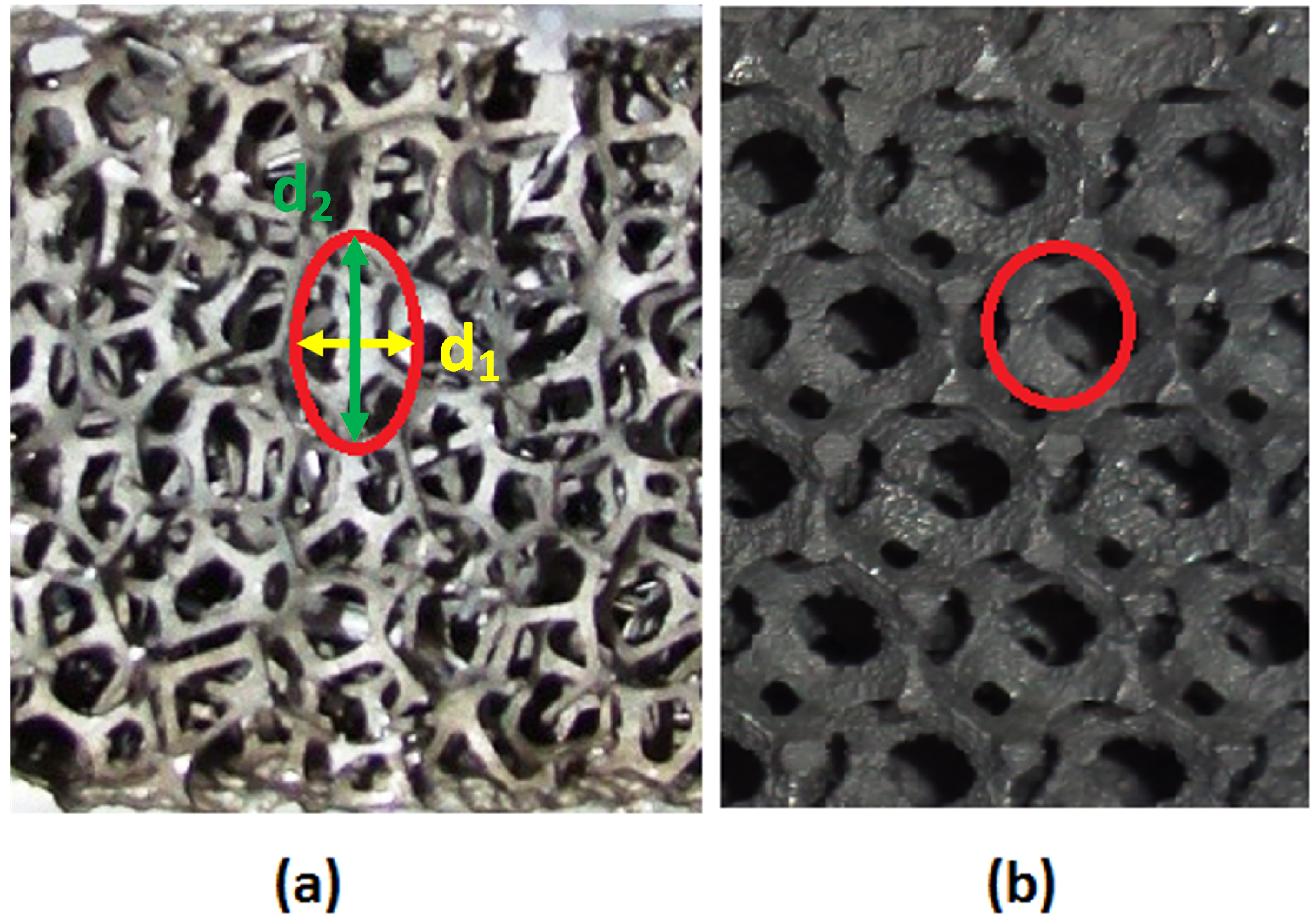
• Geometrical characterization [21]., as discussed later in this work.
• Orientation under which the metal foam sample is placed [22]: Metal foam is generally not isotropic, depending on the manufacturing technique.
• Bonding methods [23]: Commonly, this is achieved with a high conductive epoxy or by brazing/soldering. Although epoxy contact is the easiest to establish, it results in an inferior thermal contact resistance, as concluded by Sekulic et al. [24], which is especially problematic for forced convective applications.
• Cutting method [25]: Machining can result in plastic deformation of struts at the foam edges, creating a local porosity variation. This deformation will also influence the amount of struts that are available for contact with a substrate when bonded together.
• Effects of boundary conditions at the interface of a foam; especially of importance when comparing lumped parameters like permeability determined from two test sections with a completely different cross-section.
• Specific construction of the test rig.
• Effect of radiation [26]: Determination of radiative properties is of great importance in buoyancy-driven convection and high temperature applications.
• Effect of fouling.

As it would be very expensive to test the effect of all of these parameters in detail, a great deal of effort has gone to the numerical study of open-cell foam with CFD [27]. Most of the existing numerical work is done on the volume averaging theory (VAT) and the determination of the closure terms. A specific way to determine these terms will be discussed in Section 3.

Of course, most of the time, experiments and numerical work are closely linked together, as the numerical model always needs benchmarking with experiments.

This work will focus on how experiments and numerical studies should be performed, rather then focusing on all parameters influencing the thermal performance of an application. The influence of the experimental or numerical method on the repeatability of the results found in the open literature will be studied in this work. Furthermore, a new numerical method for studying open-cell metal foam will be proposed.

2. Experimental Metal Foam Studies

2.1. Usability of Experiments

The understanding, prediction and/or optimization of the thermal-hydraulic performance of thermal applications relies on solving physical models on an appropriate geometrical scale. Thermal applications for open-cell metal foam can be found in a large variety of systems and under significantly different flow alignments. It seems that for these applications, the existing research mainly consists of experimental work. In Section 1.3, many parameters to be studied for applications with open-cell foam are discussed. Due to this, experiments are time consuming. Furthermore, the results of the existing experimental work show quite a large scatter [28]. This can be largely attributed to the characterization of open-cell metal foam in the open literature, as will be explained and illustrated later on. Moreover, in many cases, not all parameters mentioned in Section 1.3 are discussed in a research paper, like the employed contact or cutting technique. For example, Chumpio and Hooman [29] mention that thermal glue was used as a contact technology. However, the authors did not specify the type of glue. In Sertkaya et al. [30], the contact technology was not reported. Hu et al. [31] mention the importance of foam boundary effects in their thermal application; however, they do not study its effects on their results.

If the experiments are done profoundly, the main advantage of experimental research is that the results are ”directly interpretable”. Of course, the quality of the experimental approach influences the quality of the results.

An essential part of a good research paper is that its results are repeatable. In this way, other authors are able to compare their results with work from the open literature. In this respect, there is much work to be done in the field of open-cell metal foam, since the authors frequently do not report a full characterization of the used foam samples, but instead only report bulk properties. As will be discussed in the next paragraph, this leads to significant scatter on the results for the performance of the metal foam.

2.2. Working with Bulk Properties

Most manufacturers characterize their metal foam products by reporting both the numbers of pores per linear inch (PPI) and the volumetric porosity ($1-\frac{m_{\mathrm{solid}}/{\rho }_{\mathrm{solid}}}{V_{\mathrm{tot}}}$). The volumetric porosity is quite easy to measure with a relatively low uncertainty of 2%–3%. In theory, the number of PPI should be quite easy to measure, as well. However, as the foam structure is inherently three-dimensional, the PPI value heavily depends on the direction in which the PPI is measured. This is also evident in Figure 3. At least three different PPI values should be reported for each foam sample, one in every dimension. Furthermore, the reported PPI values in the open literature are mostly multiples of five (5, 10, 15, etc.), which is certainly not representative of the complex and three-dimensional structure of (cast) open-cell metal foam. However, the integration of the PPI value has led to a large commercial value. For actual foam samples, these PPI values are far from a multiple of five, as can be seen in Billiet et al. [22].

The review paper by Mahjoob and Vafai [32] shows that generally, only three parameters are used in correlations for the surface-to-volume ratio and tortuosity: the volumetric porosity, PPI and an ”average fiber diameter” ($d_f$). The latter is also called the strut diameter and is measured with a microscope. However, there is no general consensus on how and where to measure $d_f$, as this fiber diameter varies over the strut length, as shown in Figure 4 for a foam made by ERG Materials and Aerospace. A detailed study of this axial variation was carried out by Jang et al. [33]. One way of dealing with this issue could be to report the location where the fiber diameter is measured (for example at $x/l=0$ in Figure 4).

Figure 4. An illustration of the axial thickness variation along the strut length for a foam made by Energy Research and Generation (ERG) [34].

Figure 4. An illustration of the axial thickness variation along the strut length for a foam made by Energy Research and Generation (ERG) [34].

In some correlations, as mentioned in the review paper by Mahjoob and Vafai [32], the average pore diameter ($d_p$) is used. This value is calculated either based on the PPI value provided by the manufacturer ($0.0254/PPI$) or through a correlation based on the average diameter. The correlation by Du Plessis et al. [35,36] for $d_p$ is a frequently-used example of such a correlation (Equation (1)). In Equation (1), $d_p$ is a function of both the tortuosity and the equivalent diameter of a cubic unit cell volume d. This equivalent diameter is a function of both fiber and pore diameter ($d=d_f+d_p$). Another frequently-used correlation for $d_p$ is made by Calmidi [37] and depends on the fiber diameter $d_f$ and the porosity ϕ (Equation (2)).

$$d=d_p\frac{2}{3-\chi }$$

(1)

$$d_f/d_p=1.18\sqrt{(1-\varphi )/(3\pi )}\times 1/(1-{\mathrm{e}}^{-(1-\varphi )/0.04})$$

(2)

Furthermore, the authors often determine the surface-to-volume ratio in experimental studies to allow for a physical interpretation of the results and/or to compare the foam sample to other fin materials, like, e.g., louvered fins. In the open literature, this surface-to-volume ratio is frequently calculated through a correlation like the one by Calmidi and Mahajan [38] (requiring the fiber diameter $d_f$, the pore diameter $d_p$ and the porosity ϕ) or the one by Fourie and Du Plessis [36] (depending on the tortuosity χ of the foam sample and the equivalent diameter d); see Equation (3) and Equation (4), respectively. In case of the correlation by Fourie and Du Plessis [36] is used, the tortuosity χ is also required and again calculated through a correlation (see Equation (5)) [35].

Both correlations are frequently used in the open literature. The paper from Calmidi and Mahajan is cited over 500 times and is still in use, as can be seen from these recent citations: [39,40,41]. The work from Fourie and Du Plessis [36] is cited over 150 times and is generally less used recently in the open literature.

$${\sigma }_0=\frac{3\pi d_f}{{(0.59d_p)}^2[1-{\mathrm{e}}^{-((1-\varphi )/0.04)}]}$$

(3)

$${\sigma }_0=\frac{3}{d}(3-\chi )(\chi -1)$$

(4)

$$\frac{1}{\chi }=\frac{3}{4\varphi }+\frac{\sqrt{9-8\varphi }}{2\varphi }\times \cos [\frac{4\pi }{3}+\frac{1}{3}{\cos }^{-1}\left[\frac{8{\varphi }^2-36\varphi +27}{{(9-8\varphi )}^{3/2}}\right]]$$

(5)

Other methods exist to (more effectively) determine the properties of foam samples. For example, the surface-to-volume ratio ${\sigma }_0$ can be determined indirectly via the Brunauer, Emmett and Teller (BET) method [42]. This is a technique based on the gas adsorption/desorption at the interfacial surface area. With this method, the entire surface area down to the nanometer scale is measured. This means that the BET method can be used for analyses at the nanometer scale only. However, thermal analysis is performed on a continuum scale. It is important to note that the continuum assumption is only valid when the Knudsen number is smaller than 0.01 [43]. Consequently, for the continuum hypothesis to hold, the smallest characteristic dimension that can be considered is around 5 μm. Hence, the BET method will result in too large surface areas for the intended analysis [44], as nanometer scale variations do not influence the continuum scale behavior.

The BET method is also used by ERG Materials and Aerospace for calculating their surface-to-volume ratio ${\sigma }_0$ as reported on their website. In turn, this ${\sigma }_0$ value from ERG Materials and Aerospace is often cited by authors [45], disregarding the fact that this is a strong overestimation of the actual value relevant for thermal applications [34,44].

Another very powerful method to characterize the foam is by using micro tomography ($\mu CT$) scanning. This method has recently gained some interest, as many papers dealing with this topic are emerging [46,47,48,49]. However, it is still not common practice to use it.

The following paragraph will show why neither correlations nor the BET method can be used to characterize bulk properties for the foam. The accuracy of the correlations is far less than that from a $\mu CT$ scan.

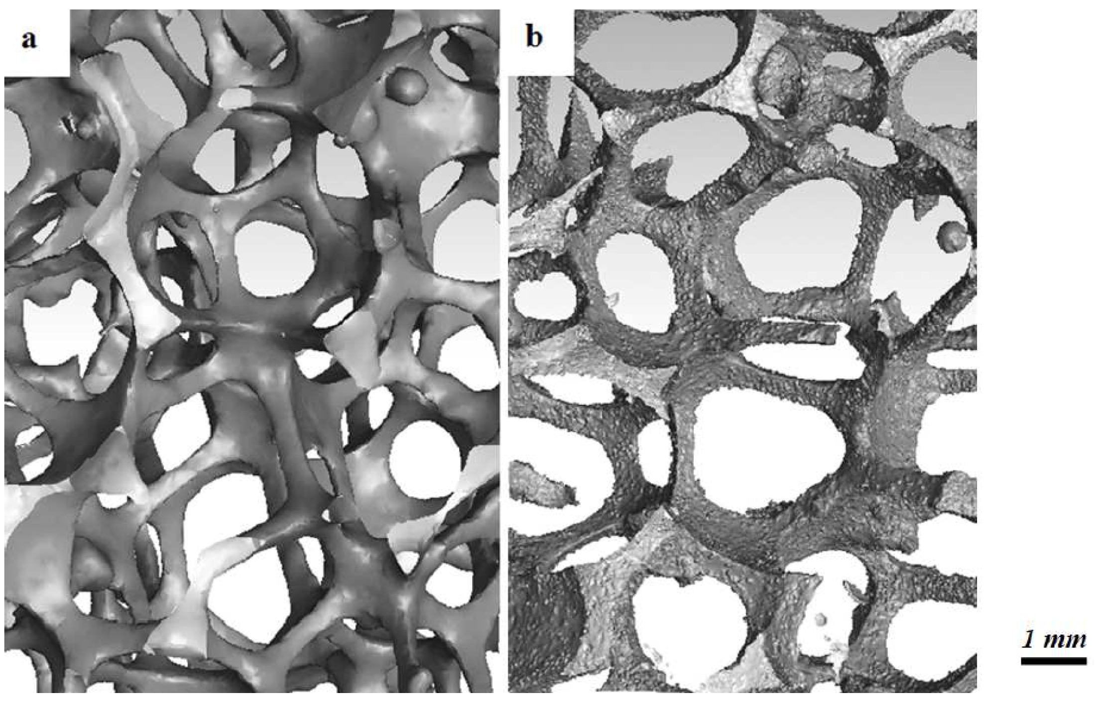
2.3. Working with Micro Tomography

A $\mu CT$ scan virtually divides the solid structure in slices with equal thickness. Each slice is divided into a number of three-dimensional pixels, which are known as voxels. Each voxel is appointed a grey value, which depends on the interaction of X-rays with the material in that voxel. After stacking the digital slices in a full three-dimensional model, the foam’s structure can be determined. Once a virtual structure is available, structural characteristics can be obtained in a systematic way through image processing techniques and dedicated algorithms.

The X-rays used in the scanning equipment interact significantly different with a solid than with a fluid (or vacuum), allowing for a clear distinction between both phases. However, voxels at the solid-fluid interface contain both phases. Therefore, their grey values can span a large range. For further image processing, they need to be binarized, i.e., allocated to either the solid (one) or fluid (zero) phase. This operation is called grey scale segmentation or thresholding [50]. An overview of different segmentation algorithms is given by Linquist [51] and recently by Ohser et al. [52]. In this work, the algorithm is based on a so-called dual threshold, which defines a threshold interval, combined with a labeling operation [53]. This means that neighboring voxels with grey values within the threshold interval are treated as a subset and are all assigned to a phase. The phase assignment is done by comparing grey values with the averaged threshold level of the interval. Grey values smaller than this averaged value are assigned to the fluid phase, while voxels with larger values are considered as solid material. This algorithm is also used in this work. For a more detailed description of the use of this technique to obtain, e.g., surface-to-volume ratios, the reader is referred to the work of De Jaeger et al. [25]. A drawback of these $\mu CT$ scans is that they are quite expensive and not straightforward to use in comparison with a microscope or the naked eye. The main difficulty lies in the choice of the averaged threshold level to allocate the voxels to either the solid (one) or fluid (zero) phase. A different threshold can yield significantly different allocations of fluid volumes [34] and, thus, a significantly different foam model. Furthermore, the voxel size itself can also significantly influence the results (as shown in Figure 5). Figure 5a is constructed with a voxel size of 37.5 μm, while Figure 5b, which clearly shows more detail, is made through a scan with a voxel size of 8.5 μm. The surface-to-volume ratio of both reconstructions in Figure 5 is respectively 720 and 860 m${}^{-1}$: a relative difference of 19%. The scan here is done on at least 16 foam cells. The reported values are average ones. This shows that the voxel size, next to thresholding, is an important parameter [25]. The heat transfer performance of a fixed volume of metal foam is determined by the product of the heat transfer coefficient and the surface-to-volume ratio. The heat transfer coefficient is determined based on the measured performance and the determined surface-to-volume ratio. As long as the thermal performance is reconstructed using the same surface-to-volume ratio that was used to determine the heat transfer coefficient, the correct thermal performance will be obtained.

However, it is clear that the geometry obtained with a 37.5 μm voxel size and a 8.5 μm voxel size is fundamentally different on the continuum scale. This leads to the question whether this continuum scale roughness has a significant impact on the pressure drop and heat transfer behavior. Generally, this is not the case, as long as the flow is laminar or the roughness peaks are smaller than the thickness of the viscous sublayer in turbulent flow [54]. For numerical simulations, the relevant surface-to-volume ratio is the one obtained on a scale that does not resolve the roughness effects that do not influence the flow.

Schmierer and Razani [55] scanned metal foam samples with four different voxel sizes, ranging from 115 down to 58 μm. They found an asymptotically converging surface-to-volume ratio. Another restriction on the voxel size is imposed by the continuum assumption with no-slip boundary conditions, upon which thermal and hydraulic analysis are commonly based (as is the case for this work). Due to the continuum hypothesis to hold and with air as a working fluid, it is not necessary to have a finer spatial discretization than voxel sizes in the order of 5 μm. As a result, the high resolution scan with a voxel size of 8.5 μm of Figure 5b can be considered highly accurate [25].

Figure 5. An illustration of the effect of voxel size for a $\mu CT$ scan reconstruction with respectively a (a) 37.5 μm and a (b) 8.5 μm voxel size. Foam samples are made in-house.

Figure 5. An illustration of the effect of voxel size for a $\mu CT$ scan reconstruction with respectively a (a) 37.5 μm and a (b) 8.5 μm voxel size. Foam samples are made in-house.

$\mu CT$ scans can be used for a full characterization of the foam sample. However, some authors, like De Jaeger et al. [56], use a hybrid model. For this model, both cell diameters ($d_1$ and $d_2$, as indicated in Figure 3a) and the interfacial strut area ($A_0$) are measured with a $\mu CT$ scan. This interfacial strut area is the average cross-sectional area in the center of the strut ($x/l=0$ in Figure 4). The interfacial strut area shows a difference of merely 4% as the voxel size is reduced from 37.5 μm to 8.5 μm and is therefore not strongly influenced by the roughness. An extensive explanation on how this interfacial strut area can be calculated from $\mu CT$ data can be found in [34]. With these three parameters, the authors were able to make a model of the complete foam structure. Based on that structure, the porosity and the surface-to-volume ratio can be calculated numerically. This allows the continuum scale roughness, which is resolved by the fine $\mu CT$ scan to be neglected, for it does not contribute to the heat transfer performance. This is a hybrid model that calculates the porosity and surface-to-volume ratio based on $d_1$, $d_2$ and $A_0$, instead of using a correlation to obtain the surface-to-volume ratio ${\sigma }_0$ or performing a full characterization of the foam sample through a $\mu CT$ scan. The surface-to-volume ratio with this hybrid model for the foam studied in Figure 5 is 859 m${}^{-1}$. This is very close to the value obtained by $\mu CT$ with a voxel size of 8.5 μm (860 m${}^{-1}$). This once again indicated the necessity of using small voxel sizes.

It is worthwhile to mention that cell diameter analysis for example can also be done via scanning electron microscope (SEM), as applied by Zhou et al. [57]. In this method, foam samples are prepared by filling them with a resin, i.e., cold mounting, and are then polished. The polished side is viewed under a microscope, allowing one to perform image analysis. This method is two-dimensional in nature, making it more prone to measurement errors. However, when done with care, it allows obtaining results that are in excellent agreement with $\mu CT$ scans [57].

2.4. Comparison of Correlations, Models and Full Characterization through Micro Tomography

Properties that can be measured through $\mu CT$ scans are, e.g., porosity (ϕ), surface-to-volume ratio (${\sigma }_0$), cell diameters ($d_1$, $d_2$), pore diameter ($d_p$) and axial variation of the strut thickness. For five foam samples, the values measured with a $\mu CT$ scan are reported in Table 1. $A_0$ is the interfacial strut area as measured in the middle of the strut. The relative experimental uncertainty on the porosity and surface-to-volume ratio is at most 2 and 8%, respectively. The reported properties are also averaged properties, as the $\mu CT$ scan is performed over 16 cells of the foam sample. The surface-to-volume ratio (${\sigma }_0$) is calculated via the marching cube algorithm, as described by Lindblad [58]. The interfacial strut area ($A_0$) is calculated as described in De Jaeger et al. [56].

Note that all uncertainties in this work are expressed as 95% confidence intervals. Uncertainties are calculated according to Moffat [59].

In Table 2, a comparison is made with the correlations for the surface-to-volume ratio from Calmidi and Mahajan [38] and Fourie and Du Plessis [36]. For this comparison, the porosity and pore diameter from in-house $\mu CT$ scans are used (Table 1) together with correlations for the surface-to-volume ratio, fiber diameter and tortuosity, as reported in [35] and [37]. Furthermore, a comparison with the work of De Jaeger et al. [56], the so-called hybrid model, is also made in Table 2.

Table 1. Properties of studied foam samples, determined through a $\mu CT$ scan with a voxel size of 8.5 μm [56]. All reported foam samples were made in-house.

Foam	PPI	ϕ	$d_1$	$d_2$	$A_0$	${\sigma }_0$	$d_p$
		−	(mm)	(mm)	($\times {10}^{-1}$mm${}^2$)	(mm${}^{-1}$)	(m)
1	10	0.932 ± 0.02	4.22 ± 0.18	6.23 ± 0.18	0.998 ± 0.08	462 ± 35	2.56 ± 0.13
2	10	0.951 ± 0.02	4.28 ± 0.13	6.42 ± 0.13	0.615 ± 0.13	380 ± 30	2.61 ± 0.11
3	20	0.913 ± 0.02	2.52 ± 0.06	3.78 ± 0.06	0.463 ± 0.04	860 ± 69	1.53 ± 0.05
4	20	0.937 ± 0.02	2.77 ± 0.05	4.15 ± 0.05	0.377 ± 0.05	720 ± 58	1.69 ± 0.05
5	20	0.967 ± 0.02	2.6 ± 0.05	3.67 ± 0.05	0.126 ± 0.02	580 ± 46	1.55 ± 0.05

Table 1. Properties of studied foam samples, determined through a $\mu CT$ scan with a voxel size of 8.5 μm [56]. All reported foam samples were made in-house.

Foam	PPI	ϕ	$d_1$	$d_2$	$A_0$	${\sigma }_0$	$d_p$
		−	(mm)	(mm)	($\times {10}^{-1}$mm${}^2$)	(mm${}^{-1}$)	(m)
1	10	0.932 ± 0.02	4.22 ± 0.18	6.23 ± 0.18	0.998 ± 0.08	462 ± 35	2.56 ± 0.13
2	10	0.951 ± 0.02	4.28 ± 0.13	6.42 ± 0.13	0.615 ± 0.13	380 ± 30	2.61 ± 0.11
3	20	0.913 ± 0.02	2.52 ± 0.06	3.78 ± 0.06	0.463 ± 0.04	860 ± 69	1.53 ± 0.05
4	20	0.937 ± 0.02	2.77 ± 0.05	4.15 ± 0.05	0.377 ± 0.05	720 ± 58	1.69 ± 0.05
5	20	0.967 ± 0.02	2.6 ± 0.05	3.67 ± 0.05	0.126 ± 0.02	580 ± 46	1.55 ± 0.05

Table 2. Surface-to-volume ratio ${\sigma }_0$ results for correlations and model in the open literature for the foam samples shown in Table 1.

Foam	${\sigma }_0$ ($\mu CT$)	Calmidi and Mahajan [38]	Fourie and Du Plessis [36]	De Jaeger et al. [56]
	(m${}^{-1}$)	(m${}^{-1}$)	(m${}^{-1}$)	(m${}^{-1}$)
1	462 ± 35	1062	528	482
2	380 ± 30	884	462	403
3	860 ± 69	2000	951	860
4	720 ± 58	1549	781	694
5	580 ± 46	1218	669	573

Table 2. Surface-to-volume ratio ${\sigma }_0$ results for correlations and model in the open literature for the foam samples shown in Table 1.

Foam	${\sigma }_0$ ($\mu CT$)	Calmidi and Mahajan [38]	Fourie and Du Plessis [36]	De Jaeger et al. [56]
	(m${}^{-1}$)	(m${}^{-1}$)	(m${}^{-1}$)	(m${}^{-1}$)
1	462 ± 35	1062	528	482
2	380 ± 30	884	462	403
3	860 ± 69	2000	951	860
4	720 ± 58	1549	781	694
5	580 ± 46	1218	669	573

Both Table 1 and Table 2 show that the results from correlations show a large deviation from the results obtained through a $\mu CT$ scan. The correlation of Calmidi and Mahajan [38] is the least accurate with differences up to 233%. Furthermore, the correlation of Fourie and Du Plessis [36] deviates up to 22% from the experimental results of the full $\mu CT$ data. Furthermore, note that both correlations consistently overestimate the measured surface-to-volume ratio at the 8.5-μm scale. As previously discussed, the surface-to-volume ratio at this scale is actually already an overestimation of the surface-to-volume ratio, which is relevant for the heat transfer and pressure drop. However, these correlations are often used in the open literature [60]. Furthermore, also notice that the comparison made in Table 2 is based on input parameters that are determined through $\mu CT$ and not according to the common practice as discussed in the paper of Mahjoob and Vafai [32]. As a result, the deviations will be even higher if the uncertainty on the input parameters for the correlations are larger, such as when they are determined through a microscope or the naked eye. This will not only influence the repeatability of the experiments, it will also influence the results. Both in numerical and experimental work, parameters as ${\sigma }_0$ are used as input.

Furthermore, the results from the model of De Jaeger et al. [56] show a much better agreement with the $\mu CT$ scan data. With a relative uncertainty level of 10% [56], the values for ${\sigma }_0$ match the experimental values.

However, $\mu CT$ scan data are still necessary in the model of De Jaeger et al. [56] as the input parameters ($d_1$, $d_2$ and $A_0$) need to be determined. Hence, the method by De Jaeger et al. [56] requires a great amount of effort. Yet, with the currently available correlations, $\mu CT$ scans (or the SEM method) are the only way to ensure a relative error that is smaller than 10%.

As will be discussed later, the pressure drop of the metal foam can be characterized by the permeability and the inertial coefficient. These quantities in turn are mainly determined by the geometric foam properties that have been discussed so far. Since it has been shown that the uncertainty on these geometrical properties is rather large, it is not surprising that a large discrepancy can be found between the experimental results for the permeability and inertial coefficient in the open literature [28]. Furthermore, the smaller the mass flow rate, the larger the discrepancies. These properties are frequently seen as bulk properties of the porous medium. In Section 3.2.2 of this manuscript, these properties will be discussed more extensively. Next to the geometrical characterization of the foam, there are also other factors that determine the permeability and inertial coefficient: interpolation details, wall boundary layer effects, entrance/exit effects, dependency of the velocity range over which the quadratic correlation is taken to calculate permeability and the inertial coefficient, for example [34]. However, these parameters (permeability and inertial coefficient) are also used in numerical calculations or experimental investigations, as shown by the recent review by Yang et al. [61]. The uncertainty on the permeability and the inertial coefficient will result in an uncertainty on the performance of the metal foam.

As will be explained in the next section, numerical work could be a solution in order to determine permeability and the inertial coefficient more profoundly.

3. Numerical Work: The Volume Averaging Theory

Based on the previous paragraph, it is clear that proper characterization is necessary to make the data in the literature repeatable for other authors. Based on the discussion in Section 1.3, it is also clear that numerical simulations are required due to the large number of parameters influencing the thermohydraulics in open-cell metal foam. Studying complete metal foam applications numerically by, e.g., direct numerical simulation (DNS) is not feasible, because this requires a very large amount of computational time, as these simulations require tens of millions of computational cells for a single foam cell [62]. The other extreme is an experiment. From Section 1.3, it is clear that there are many parameters to investigate, which is also very time consuming. Therefore, there is a need for an efficient and accurate method to study macro-scale models numerically. There are many methods that can be used for porous media, like the one based on the homogenization theory or through the stochastic method [63]. However, the focus in this work will be on the the volume averaging theory (VAT) [64]. Parts of this work are reported in the PhD thesis of Peter De Jaeger (co-author of this work) [34].

3.1. From the Micro- to the Macro-Scale

The volume averaging theory starts with the microscopically-scaled model. Equations (6)–(9) form the well-known Navier-Stokes equations for a thermal non-equilibrium model, without heat generation.

$$\begin{array}{ccc}\hfill \nabla ·\overrightarrow{v}& =& 0\hfill \end{array}$$

(6)

$$\begin{array}{ccc}\hfill {\rho }_f\frac{\partial \overrightarrow{v}}{\partial t}+{\rho }_f\nabla ·(\overrightarrow{v}\overrightarrow{v})& =& -\nabla P+{\mu }_f{\nabla }^2\overrightarrow{v}+{\rho }_f\overrightarrow{g}\hfill \end{array}$$

(7)

$${(\rho c_p)}_f\left[\frac{\partial T_f}{\partial t}+\overrightarrow{v}·\nabla T_f\right]=k_f{\nabla }^2{T}_f$$

(8)

$${(\rho c_p)}_s\frac{\partial T_s}{\partial t}=k_s{\nabla }^2{T}_s$$

(9)

In these equations, $\overrightarrow{v}$ (m/s) is the local velocity vector, ${\rho }_f$ (kg/m${}^3$) the fluid density, P (Pa) the pressure, ${\mu }_f$ (kg/(m·s)) the dynamic viscosity of the fluid saturating the porous medium, $\overrightarrow{g}$ (m/s${}^2$) the gravitational acceleration, $c_{p_f}$ (J/(kg·K)) the specific heat of the fluid phase, $k_f$ (W/(m·K)) the fluid thermal conductivity, $T_f$ (K) the fluid phase temperature, with $c_{p_s}$ (J/ (kg·K)) the specific heat of the solid phase, $k_s$ (W/(m·K)) the solid thermal conductivity and $T_s$ (K) the solid phase temperature.

The macroscopic scale is a linear dimension of a representative elementary volume (REV) as defined by Bear [65]. Following Cushman et al. [66], the existence of the macroscopic scale makes open-cell foam a discrete hierarchical material, which indicates that there exists a clear-cut length scale separation between the micro- and macro-scopically-scaled physics. It is important to note here that this implies that the averaged variables over a REV have to behave quasi-steady, compared to their continuum-scaled counterparts. The length scale separation makes it convenient to perform the upscaling via the VAT, as described by Whitaker [64]. The resulting macroscopic flow and energy equations for incompressible flow with constant fluid properties in the REV, stationary solid phase and constant porosity are then given by Equations (10)–(13) [67]. According to Minkowycs et al. [68], thermal equilibrium equations can only be used when $R{e}_{d_f}<0.1$. This means that the convection coefficient cannot be assumed to be infinitely large, and two energy equations (for the fluid and solid field) have to be solved. An interstitial convection coefficient makes the connection between the solid and fluid domain. In these equations, the closure terms $\stackrel{=}{\kappa }$, $\stackrel{=}{\beta }$, $\stackrel{=}{k_d}$ (thermal dispersion) and $h_{fs}$ (interstitial heat transfer coefficient) appear. The determination of these terms is discussed in the next paragraph. Furthermore, as can be seen from the equations, some terms are tensorial.

$$\begin{array}{ccc}\hfill \nabla ·{\langle \overrightarrow{v}\rangle }^i& =& 0\hfill \end{array}$$

(10)

$$\begin{array}{ccc}\hfill \rho \frac{\partial {\langle \overrightarrow{v}\rangle }^i}{\partial t}+\rho {\langle \overrightarrow{v}\rangle }^i·\nabla {\langle \overrightarrow{v}\rangle }^i& =& -\nabla {\langle P\rangle }^i+{\mu }_e{\nabla }^2{\langle \overrightarrow{v}\rangle }^i+\rho \overrightarrow{g}\hfill \\ & -& \mu {\stackrel{=}{\kappa }}^{-1}·{\langle \overrightarrow{v}\rangle }^i-\rho \stackrel{=}{\beta }·\left|{\langle \overrightarrow{v}\rangle }^i\right|{\langle \overrightarrow{v}\rangle }^i\hfill \end{array}$$

(11)

$$\begin{array}{ccc}\hfill \varphi {(\rho c_p)}_f\frac{\partial {\langle T_f\rangle }^i}{\partial t}+\varphi {(\rho c_p)}_f{\langle \overrightarrow{v}\rangle }^i·\nabla {\langle T_f\rangle }^i& =& \varphi \nabla ·(\stackrel{=}{k_d}+\stackrel{=}{k_{f,e}})·\nabla {\langle T_f\rangle }^i\hfill \\ & +& h_{fs}{\sigma }_0({\langle T_s\rangle }^i-{\langle T_f\rangle }^i)\hfill \end{array}$$

(12)

$$\begin{array}{ccc}\hfill (1-\varphi ){(\rho c_p)}_s\frac{\partial {\langle T_s\rangle }^i}{\partial t}& =& (1-\varphi )\nabla ·(\overline{\overline{k_{s,e}}}·\nabla {\langle T_s\rangle }^i)\hfill \\ & -& h_{fs}{\sigma }_0({\langle T_s\rangle }^i-{\langle T_f\rangle }^i)\hfill \end{array}$$

(13)

In these equations, the superscript i stands for intrinsic. For the determination of the effective properties (effective viscosity ${\mu }_e$ and both effective conductivities $\stackrel{=}{k_{f,e}}$ and $\stackrel{=}{k_{s,e}}$), the reader is referred to [34,69,70,71,72,73,74] in which these parameters are determined numerically or analytically. De Jaeger [34] has determined these effective conductivities based on his hybrid numerical model. Similar techniques for this are also discussed by Haussener et al. [69] and Ranut [71]. The numerical results obtained here are also verified by the work of Le et al. [70] using sound to measure the tortuosity. Ochoa-Tapia and Whitaker [72,73] together with Magnico [74] have studied the effective viscosity more in detail through analytical considerations and direct numerical simulations.

Using the volume averaging theory for thermal open-cell foam applications simply comes down to properly determining the closure terms.

3.2. Discussion of Closure Terms

The closure terms that will be discussed in this section are:

• Momentum closure terms: permeability $\stackrel{=}{\kappa }$ and inertial coefficient $\stackrel{=}{\beta }$.
• Energy closure terms: thermal dispersion $\stackrel{=}{k_d}$ and interstitial heat transfer coefficient $h_{fs}$.

Most of the time, these closure terms are determined experimentally [75] or through correlations [76] and then used in a numerical study. Examples of such a procedure can be found in Phanikumar et al. [60], Zhao et al. [77], Qu et al. [40] and DeGroot et al. [78].

In this section, a method is proposed to determine all closure terms numerically from creeping to turbulent flow. This requires a geometrical model that is representative for the metal foam’s internal structure. The most accurate model available is a virtual reproduction via a $\mu CT$ scan. The resulting REV consists of at least two cells of the metal foam in each direction [50], thus containing eight cells in total. This can be done for example through the hybrid model of De Jaeger et al. [56] as discussed in Section 2.3. Of course, this hybrid model is not the exact geometrical representation of the foam structure, but as illustrated by Table 2, it gives a very good approximation.

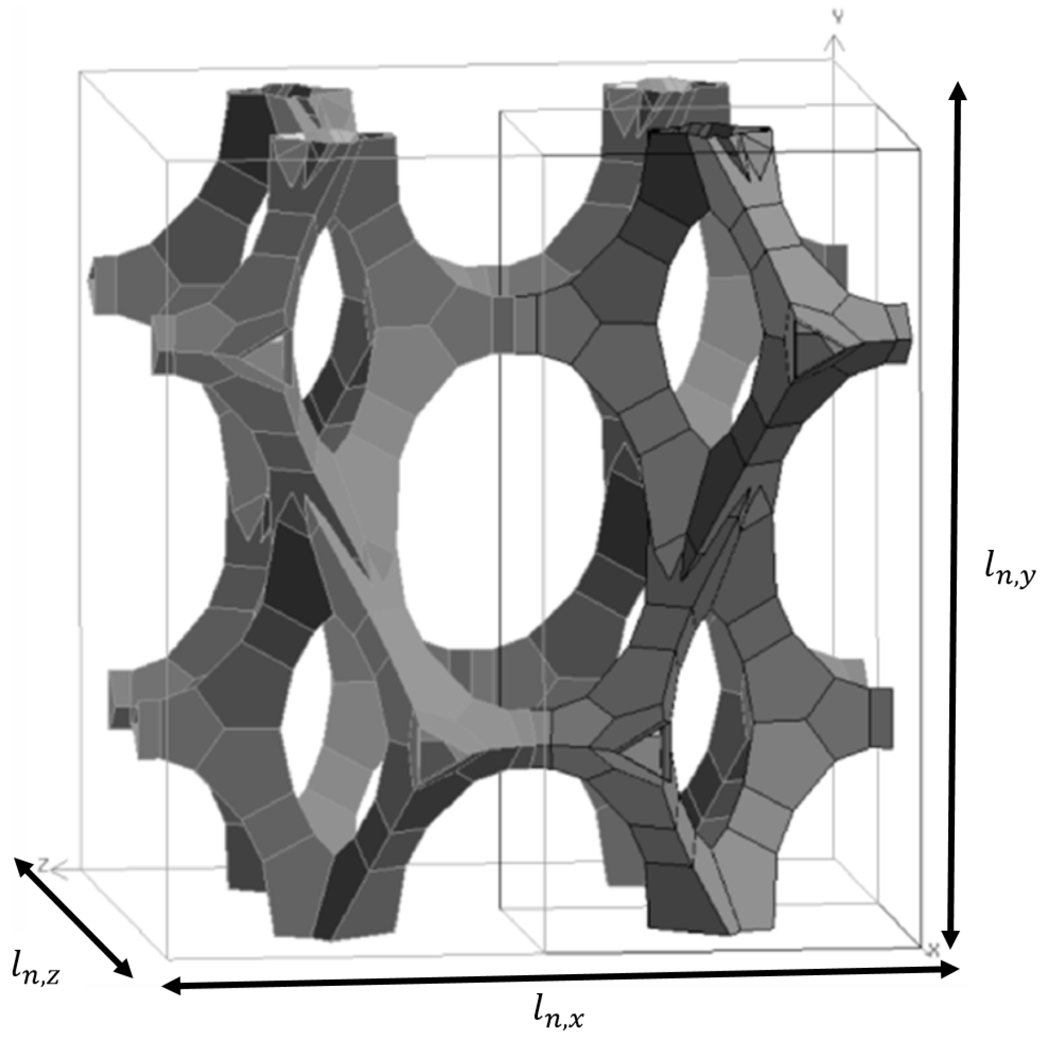
3.2.1. Foam Sample and Mesh

If a full REV, containing eight foam cells, is used, the number of numerical cells will be very high. For example, to mesh Foam 1 from Table 1 with a minimum start size of 8 μm [79] and a growth rate of 1.1, the number of cells will be in the order of 200 million. This is insolvable without having a supercomputer available.

A solution for this problem can be found by using the $\mu CT$ data of approximately 30 foam cells. Based on these data, an average value is determined for $d_1$, $d_2$ and $A_0$. With these values, the model of De Jaeger et al. [56] is used to reproduce a periodic unit foam cell (PUC) as shown in Figure 6. This is only one unit foam cell instead of eight foam cells. The fluid domain around this foam cell is then meshed with a first layer thickness of 8 μm and a growth rate of 1.1, resulting in 31 million numerical cells for Foam 1 in Table 1. This is more manageable than the 200 millions numerical cells for a full representative elementary unit cell.

To generate the computational grid with periodic boundary conditions, matching grid spacing is required on the periodic faces (which is known as conformal). The software used however only allows this in two directions. Another possibility is defining the periodic bounding faces of the computational domain as interfaces. This allows linking the periodic faces, later in the solver. The drawback of the latter solution though is that values from one bounding face need to be interpolated to yield the values of the non-matching periodic face; this is generally denoted by ”non-conformal meshing” in computational fluid dynamics.

Figure 6. An illustration of a periodic unit cell from the model of De Jaeger et al. [56] (Foam 1 from Table 1).

Figure 6. An illustration of a periodic unit cell from the model of De Jaeger et al. [56] (Foam 1 from Table 1).

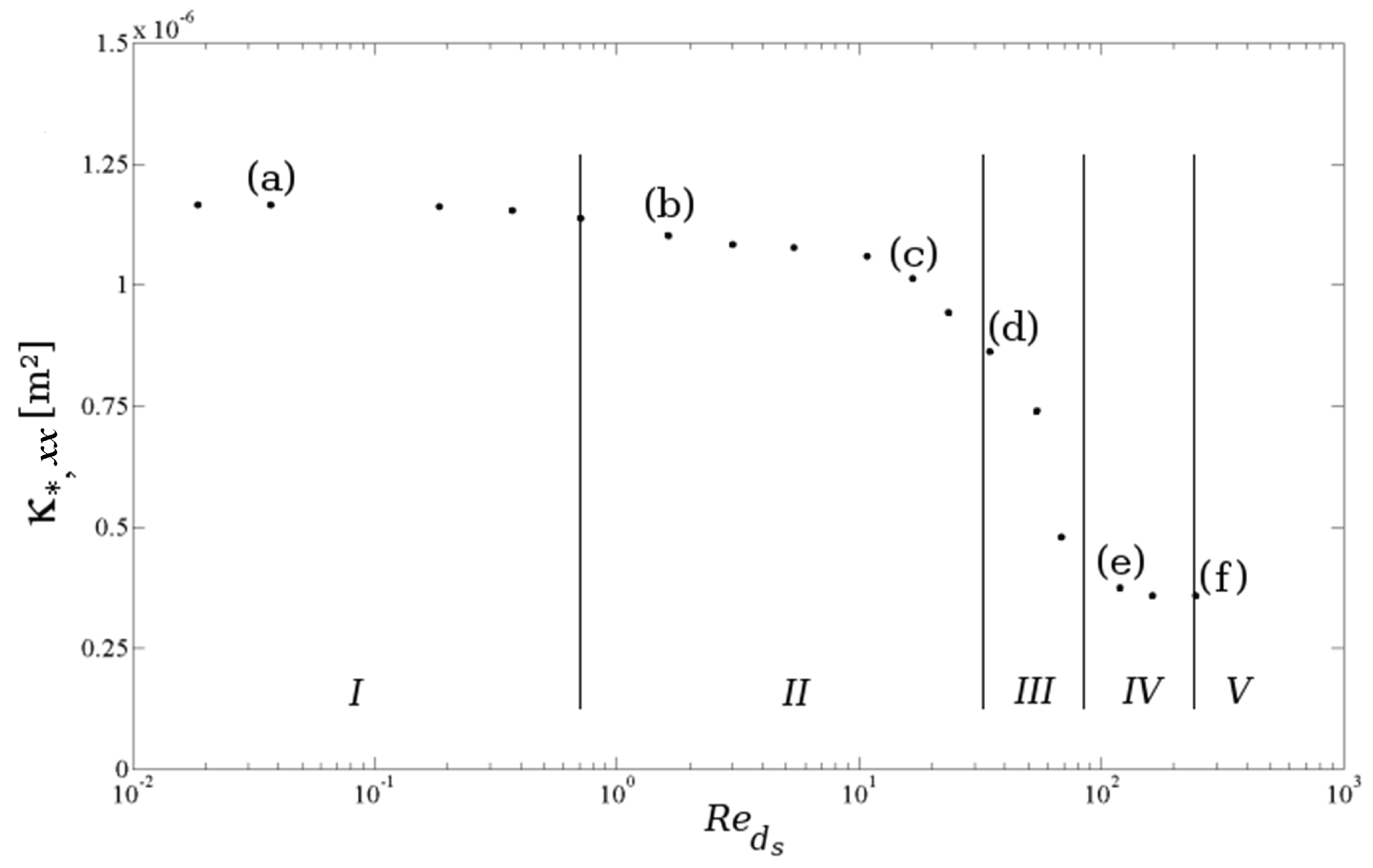
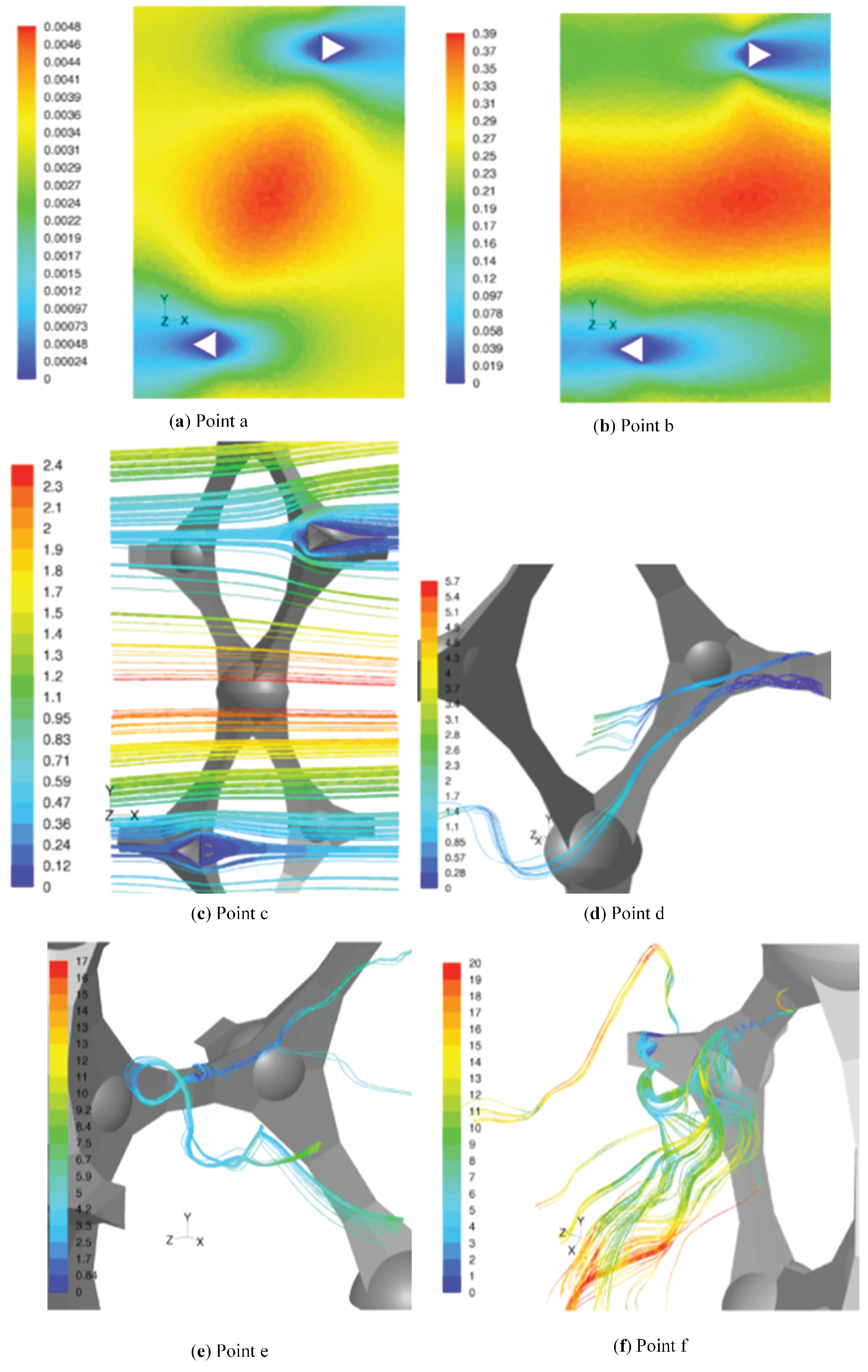
3.2.2. Momentum Closure Terms

The textbook of Whitaker [80] describes what the volume averaged momentum equations look like. In case of no-penetration and no-slip boundary conditions near the solid-fluid interface, this results in a pressure drag and a viscous drag force. For a macroscopically-steady and fully-developed flow, Equation (11) reduces to Equation (14) according to the findings of Gray [81]. This equation will be taken as a starting point for the determination of the momentum closure terms.

$$\begin{array}{ccc}\hfill \nabla {\langle P\rangle }^i& =& -\frac{1}{V_m}{\int }_{A_{fs}}{\overrightarrow{n}}_{fs}(\tilde{P}I+\mu \nabla \tilde{\overrightarrow{v}})dA\hfill \end{array}$$

(14)

Whitaker [80,82] theoretically showed that closing Equation (11) results in the Darcy-Forchheimer equation. Whitaker applied the general closure modeling scheme on the macroscopic continuity and momentum balance equation, in order to close both integral terms in the latter. The spatial deviation terms are mapped on the intrinsic velocity according to:

$$\begin{array}{ccc}\hfill \tilde{\overrightarrow{v}}& =& \stackrel{=}{M}·{\langle \overrightarrow{v}\rangle }^i\hfill \\ \hfill \tilde{P}& =& \mu \overrightarrow{m}·{\langle \overrightarrow{v}\rangle }^i\hfill \end{array}$$

Substituting these mapping functions in the closure problem and recognizing that ${\langle \overrightarrow{v}\rangle }^i$ is quasi-constant in an REV (which is the measurement window $V_m$), the closure problem can be re-written, such that it requires solving for the two mapping functions $\stackrel{=}{M}$ and $\overrightarrow{m}$. An additional step was issued by Whitaker, which provides a theoretical framework for the derivation of the Darcy-Forchheimer equation. This step is needed because the first mapping function is fully related to the viscous drag, while the second mapping is related to the form drag effect. The permeability and inertial factor in the phenomenological Darcy-Forchheimer equation though are influenced by both effects. Therefore, the mapping functions need to be split and blended into new mapping functions, in order to resemble the phenomenologically-defined permeability and inertial loss factor. It should be mentioned that this theoretical development of the Darcy-Forchheimer equation still requires solving the microscopic flow phenomena on a periodic unit cell representation of the solid phase, and this in such a fashion that the mapping functions can be derived. Nevertheless, it is clear that the Darcy-Forchheimer equation is a proper closure model for the viscous and pressure drag.

These properties are defined for macroscopically fully-developed and steady flow. The re-arranged VAT-based now read:

$$\begin{array}{ccc}\hfill -\varphi \nabla {\langle P\rangle }^i& =& -1/V_m{\int }_{A_{fs}}\mu \nabla \tilde{\overrightarrow{v}}(\overrightarrow{r})·{\overrightarrow{n}}_{fs}dA+1/V_m{\int }_{A_{fs}}\tilde{P}(\overrightarrow{r}){\overrightarrow{n}}_{fs}dA\hfill \end{array}$$

(15)

In Equation (15), the subscript fs stands for solid-fluid interface and $\overrightarrow{n}$ for the unit vector normal to the respective surface. Next to Equation (14), the most widely-used equation for momentum transport is the Darcy-Forchheimer equation (or Hazen-Dupuit-Darcy equation) shown in Equation (16) [83,84].

$$-\nabla {\langle P\rangle }^i=\frac{\mu }{\stackrel{=}{\kappa }}{\langle \overrightarrow{v}\rangle }^i+\rho \stackrel{=}{\beta }\left|{\langle \overrightarrow{v}\rangle }^i\right|{\langle \overrightarrow{v}\rangle }^i$$

(16)

Comparing this equation to Equation (16), the permeability and inertial loss factor (in tensorial form) are given by Equations (17) and (18).

$$\begin{array}{ccc}\hfill {\langle \overrightarrow{v}\rangle }^s{\stackrel{=}{\kappa }}_{*}^{-1}& =& \frac{1}{\mu }\frac{1}{V_m}{\int }_{A_{fs}}\mu \nabla \tilde{\overrightarrow{v}}(\overrightarrow{r})·{\overrightarrow{n}}_{fs}dA\hfill \end{array}$$

(17)

$$\begin{array}{ccc}\hfill {\langle \overrightarrow{v}\rangle }^s{\stackrel{=}{\beta }}_{*}& =& \frac{1}{\rho |{\langle \overrightarrow{v}\rangle }^s|}\frac{1}{V_m}{\int }_{A_{fs}}\tilde{P}(\overrightarrow{r}){\overrightarrow{n}}_{fs}dA\hfill \end{array}$$

(18)

In Equations (17) and (18), the superscript s stands for superficial and subscript m for measuring (volume). Recognizing that the integrals in these equations are respectively the viscous and the pressure force that act on the fluid-solid interface gives a physical interpretation to both parameters. The subscript asterisk indicates that both properties are determined by a direct numerical formation. Indeed, a distinction needs to be made with the phenomenologically-defined permeability $\stackrel{=}{\kappa }$ and inertial coefficient $\stackrel{=}{\beta }$. These phenomenological parameters are described as a material property and assumed to be independent of the velocity. In contrast, in the numerical simulation, no assumptions are made on the dependency of these properties on the velocity. The only assumption that is invoked is that the permeability results from the viscous forces, and the inertial coefficient results from the pressure forces. Note that in a macroscopically fully-developed and steady flow, the momentum balance becomes a pure force balance between the pressure gradient and the drag forces that act on the interstitial surface. Therefore, one could argue the need to characterize both drag forces separately via porous properties, i.e., why not give a direct dependency between the total drag force and the geometrical characteristics? One reason is that both the permeability and inertial coefficient found are widely used amongst engineers.

Based on this idea, one can calculate permeability and the inertial coefficient by applying different pressure gradients in each direction; ranging for example from 0.05–50 kPa/m. For this unsteady calculation, the computational time is quite high. It takes one month to calculate the data on a Dell (Round Rock, TX, USA) machine with dual hex core Xean X5690 3.46-GHz processors with 12 MB Cache and an on-board memory of 96 GB DDR3-1333 MHz RAM. However, this calculation only has to be done once. In Figure 7 and Figure 9, the results for the x-direction are shown. It is apparent that both properties depend on the Reynolds number. The characteristic length for the Reynolds number reported here is the strut diameter ($d_s$), which is based on the interfacial strut area in the middle of the strut ($A_0$ as reported in the work of De Jaeger et al. [56]). The characteristic velocity in the Reynolds number is the superficial velocity.

Figure 7. Permeability (${\kappa }_{*,xx}$) versus Reynolds number for Foam 1 in Table 1. The five flow regimes are indicated (I–V).

Figure 7. Permeability (${\kappa }_{*,xx}$) versus Reynolds number for Foam 1 in Table 1. The five flow regimes are indicated (I–V).

Figure 8. Illustration of the different flow regimes as indicated in Figure 7 and Figure 9. (a) Point a: $R{e}_{d_s}=0.038$; (b) Point b: $R{e}_{d_s}=1.67$; (c) Point c: $R{e}_{d_s}=16.9$; (d) Point d: $R{e}_{d_s}=36.0$; (e) Point e: $R{e}_{d_s}=105.3$; (f) Point f: $R{e}_{d_s}=249.9$.

Figure 8. Illustration of the different flow regimes as indicated in Figure 7 and Figure 9. (a) Point a: $R{e}_{d_s}=0.038$; (b) Point b: $R{e}_{d_s}=1.67$; (c) Point c: $R{e}_{d_s}=16.9$; (d) Point d: $R{e}_{d_s}=36.0$; (e) Point e: $R{e}_{d_s}=105.3$; (f) Point f: $R{e}_{d_s}=249.9$.

Figure 9. Inertial coefficient (${\beta }_{*,xx}$) versus Reynolds number for Foam 1 in Table 1.

Figure 9. Inertial coefficient (${\beta }_{*,xx}$) versus Reynolds number for Foam 1 in Table 1.

For the first three points ((a)–(c)) in Figure 7, the flow is laminar and steady. For the lowest Reynolds number, Point (a), an inertial core starts to form in the pores. The core does not span the complete flow domain and, therefore, has no influence on the struts downstream (see Figure 8a). This changes for the second point (b) (see Figure 8b), where the inertial core now spans the complete flow region. The permeability shows a slight decrease, as can be seen in Figure 7. Recalling the relation between permeability and viscous drag force, this decrease in permeability implies that the strain rate (and thus, the shear stress for a Newtonian fluid) increases more than the intrinsic velocity increases, i.e., the effect of the inertial core formation is felt downstream in the foam sample.

In the third steady-laminar case, Point (c) in Figure 7, recirculation zones are formed in the wake behind the struts (see Figure 8c). Note that in an actual foam sample, where the struts are not well aligned, as in the idealized PUC representation, this formation of recirculation zones can be understood by recognizing that the regions containing the recirculation zones have a very limited contribution to the mass flow rate through the foam volume. On the other hand, the mass flow rate increases compared to the previous point (b). As the majority of the increase in mass flow rate has to pass through a decreased volume, the inertial core tightens. This results in a larger increase of the strain rate near the solid-fluid interface than of the filtration velocity. At Point (d), the flow has entered the unsteady laminar regime: see Figure 8d. This is slightly above the critical value of $R{e}_{d_s}=31.5$ as also reported by [74].

Increasing the Reynolds number further makes the flow enter the transitional regime, and for $R{e}_{d_s}>120$ (in this case), there is an equilibrium between the increment of filtration velocity and strain rate: permeability tends to a constant value. This is characterized by the highly unsteady flow, resembling turbulence. This is visualized in Points (e) and (f) in Figure 8.

In Figure 9, the inertial coefficient is defined as the ratio of the pressure force density to the kinetic energy of the fluid (Equation (18)). This pressure force is determined by the pressure distribution over the surface area of the solid-fluid interface. Upstream of a strut, there is a stagnation zone, where kinetic energy reduces to zero and results in a region with high pressure. Downstream, a distinction has to be made between flow regimes with or without recirculation regions in the wakes behind the struts. In case there is no circulation ($R{e}_{d_s}<10$), the inertial coefficient decreases with increasing Reynolds number. This means that the pressure force increases at a lower rate than the averaged kinetic energy in the flow domain. When the recirculation regimes in the wakes downstream the struts start to appear ($R{e}_{d_s}>10$), the increment of pressure force and averaged kinetic energy is equal. This is characterized by a nearly constant inertial loss factor.

3.2.3. Energy Closure Terms

A numerical study of the thermal dispersion term ${\stackrel{=}{k}}_d$ is performed by imposing a periodic temperature change in each direction, subjected to specified heat flux condition at the interstitial surface.

The commercial solver now assumes a constant temperature gradient (similar to the pressure gradient given in Section 3.2.2). These gradient are for the quarter-PUC given by [79]:

$$\begin{array}{ccc}\hfill \frac{T(x+\frac{l_{n,x}}{2},y,z)-T(x,y,z)}{\frac{l_{n,x}}{2}}& =& \frac{T(x+l_{n,x},y,z)-T(x+\frac{l_{n,x}}{2},y,z)}{\frac{l_{n,x}}{2}}=\frac{\Delta T}{\frac{l_{n,x}}{2}}\hfill \\ \hfill \frac{T(x,y+l_{n,y},z)-T(x,y,z)}{l_{n,y}}& =& \frac{T(x,y+2l_{n,y},z)-T(x,y+l_{n,y},z)}{l_{n,y}}=\frac{\Delta T}{l_{n,y}}\hfill \\ \hfill \frac{T(x,y,z+\frac{l_{n,z}}{2})-T(x,y,z)}{\frac{l_{n,z}}{2}}& =& \frac{T(x,y,z+l_{n,z})-T(x,y,z+\frac{l_{n,z}}{2})}{\frac{l_{n,x}}{2}}=\frac{\Delta T}{\frac{l_{n,z}}{2}}\hfill \end{array}$$

Note that the thermal dispersion term is modeled similar to momentum dispersion, through a gradient-type diffusion model. The applied gradients are constant in all three directions. When fluid flow is considered in a single direction, along the x or y coordinate, this temperature gradient is practically only significant in the applied direction. In the other directions, it can be assumed to be negligibly small. This allows specifying the constant gradient. For example, for an x directed flow, it reads:

$$\frac{\Delta T}{\frac{l_{n,x}}{2}}=\frac{\dot{q}{A}_{fs}}{\dot{m}{c}_p}\frac{1}{\frac{l_{n,x}}{2}}=\frac{T_{bulk,x=\frac{l_{n,x}}{2}}-T_{bulk,x=0}}{\frac{l_{n,x}}{2}}$$

(19)

where the subscript bulk is the mass weighted average at the indicated face.

For the determination of the thermal dispersion, it is common to consider the dispersion diffusivity ${\stackrel{=}{\alpha }}_d=\frac{{\overline{\overline{k}}}_d}{{(\rho c_p)}_f}$ (m${}^3$/s) instead of the thermal dispersion itself. It is typically assumed that this tensor is symmetrical [85]. Furthermore, its principal directions are assumed to be aligned with the small and large cell diameter. Whitaker [64] has shown that for discrete hierarchical structures, the thermal diffusivity in the x direction can be determined from the local data by applying Equation (20) [86]. The macroscopic temperature gradient ${\langle {\tilde{v}}_x\tilde{T}\rangle }^i$ is determined by ${\langle {\tilde{v}}_x\tilde{T}\rangle }^i={\langle v_{x}T\rangle }^i-{\langle v_x\rangle }^i{\langle T\rangle }^i$.

$${\alpha }_{d,xx}=-\frac{{\langle {\tilde{v}}_x\tilde{T}\rangle }^i}{\frac{\Delta T}{\frac{l_{n,x}}{2}}}$$

(20)

The method to solve this is based on the discussion of the mesh in Section 3.2.1, where it was explained that a non-conformal mesh has to be used because of the periodic boundary conditions around the PUC. Concerning the macroscopic temperature gradient in the denominator of Equation (20), the bulk temperatures are practically obtained by considering a place that is located away from the periodic planes over a distance of the dimension of one control volume. This ensures that no interpolation errors, due to the non-conformal mesh, are present.

Doing so, this results in a heat balance closure within 1.5%, between the imposed heat transfer rate at the interstitial surface and the retrieved thermal energy in the air flow.

Validation of the obtained results is done by comparing to data given in the open literature. Often cited is the work of Calmidi et al. [38], which proposed the following correlation under the assumption of isotropic foam:

$$\frac{{\alpha }_d}{{\alpha }_f}=0.06\frac{1}{{\alpha }_f}\left|{\langle \overrightarrow{v}\rangle }^i\right|\sqrt{\kappa }$$

(21)

This correlation was obtained via an inverse technique by adapting the coefficient in front of the correlation until modeled and experimental heat transfer for a given foam yield the same (thus resulting in 0.06). As can be seen from Figure 10 (red symbols), the agreement with the CFD results from this work is poor. Calmidi et al. [38], however, report a low sensitivity of their system towards the thermal dispersion and, hence, indicate that the obtained figure of 0.06 gives an order of magnitude. It allows them to assess the importance of thermal dispersion with respect to the solid phase effective thermal conductivity, which is assumed to account for the major part of conductive heat transfer in foams. It was shown that at $R{e}_{d_s}\approx 30$, thermal dispersion merely accounts for 3% of the conductive heat transfer in foam. Based on this, the authors neglect thermal dispersion for $R{e}_{d_s}<30$. For higher Reynolds numbers, thermal dispersion needs to be accounted for.

Figure 10. Validation of thermal dispersion diffusivity. The symbols + and ∘ represent respectively the $k_{d,xx}$ and $k_{d,yy}$ results. The colors distinguish between data from Calmidi et al. [38] (red), Kaviany [87] (blue), Steven et al. [88] (green) and the CFD results obtained in this work (black).

Figure 10. Validation of thermal dispersion diffusivity. The symbols + and ∘ represent respectively the $k_{d,xx}$ and $k_{d,yy}$ results. The colors distinguish between data from Calmidi et al. [38] (red), Kaviany [87] (blue), Steven et al. [88] (green) and the CFD results obtained in this work (black).

A general correlation for thermal dispersion, derived from a large amount of experimental data and for a variety of porous media, is given in the textbook of Kaviany [87]. Amongst others, it is based on the work of Koch et al. [89], which deals with metallic fibrous media. The resulting correlation reads:

$$\frac{{\alpha }_{d,xx}}{{\alpha }_f}=\frac{3}{4}Pe+\frac{1}{6}{\pi }^2(1-\varphi )PelnPe,$$

(22)

with the Peclet number given by $P{e}_{d_p}=\frac{|{\langle \overrightarrow{v}\rangle }^s|d_p}{{\alpha }_f}$. The data depicted in Figure 10 (blue symbols) is based on the appropriate Peclet number (based on the pore diameter), but shown with respect to $R{e}_{d_s}$ on the abscissa. Good agreement is found for $R{e}_{d_s}>10$. Below this Reynolds number, a major deviation is observed. Recalling the flow regimes, as treated in Section 3.2.2, this corresponds to the Reynolds number where recirculation zones in the wakes behind struts emerge. Note also that the results depicted in Figure 10 suggest that the thermal dispersion and molecular diffusion become equal at $R{e}_{d_s}\approx 10$. The same effects have been observed and reported by Steven et al. [88], in a numerical study on open-cell foams. Based on their data, they proposed the following correlation:

$$\frac{{\alpha }_{d,xx}}{{\alpha }_f}=\frac{1}{1.14}+\frac{1}{206}{\left(\frac{|{\langle \overrightarrow{v}\rangle }^i|\frac{4\varphi }{{\sigma }_0}}{{\alpha }_f}\right)}^{1.81}$$

(23)

This correlation shows good agreement with the CFD results given here, but only for $R{e}_{d_s}<10$. The large deviation for higher Reynolds numbers most likely can be attributed to the geometrical model used by these authors, which consisted of an isotropic Kelvin cell with equilateral triangular fibers representing the struts.

For calculating the interstitial heat transfer coefficient, the PUC can again be used. When imposing a constant heat flux, only two temperatures need to be computed for the determination of the interstitial heat transfer coefficient through Equation (24). This only requires determining the bulk temperature of the solid and the fluid based on the microscopic data.

$$h_{fs}=\frac{\dot{Q}}{A_{fs}({\langle T_s\rangle }^i-{\langle T_f\rangle }^i)}$$

(24)

For the solid phase temperature, further simplification is possible by considering the Biot number, given by Equation (25).

$$Bi=\frac{h_{fs}{d}_s}{k_s}$$

(25)

The Biot number gives an indication of the temperature distribution inside the struts, when they are subjected to a heat transfer towards the fluid phase. Due to the latter, the strut boundaries can be at a significantly different temperature than the solid material in the middle of the strut. For an aluminum AA4260 alloy, a conservative estimate of the heat transfer coefficient of 10 W/m${}^2$·K and a typical foam with $\varphi =0.93$ and ${\sigma }_0=500$ m${}^{-1}$, the resulting Biot number is smaller than ${10}^{-4}$. Hence, it can be safely assumed that knowing the mean interstitial surface temperature is a sufficiently accurate representation of the intrinsically averaged solid phase temperature. For this reason, it is not required to solve the conjugate heat transfer problem. $h_{fs}$ is thus given by Equation (26).

$$h_{fs}=\frac{\dot{Q}}{A_{fs}({\langle T_{fs}\rangle }^{fs}-{\langle T_f\rangle }^i)}$$

(26)

In this equation, ${\langle T_f\rangle }^i$ is easily subtracted from the microscopic simulation. ${\langle T_{fs}\rangle }^{fs}$ denotes the mean interstitial surface temperature given by Equation (27).

$${\langle T_{fs}\rangle }^{fs}=\frac{1}{A_{fs}}{\int }_{A_{fs}}{T}_{fs}dA$$

(27)

Again, this closure term depends on the Reynolds number and is tensorial.

From the large number of Nusselt correlations, published for open-cell foams (see, e.g., [32,90,91] for a survey on the subject), a correlation that strongly resembles the correlation for a bank of staggered tubes [92] is found appropriate. Experimental validation for this is offered by Calmidi et al. [38], Ghosh [93] and Tamayol et al. [94]. The appropriate correlation of Zukauskas [92] is given by Equation (28).

$$Nu=0.52R{e}_{d_s}^{0.5}P{r}^{0.37}$$

(28)

Figure 11. Validation of the interstitial heat transfer coefficient. The symbols + and ∘ represent respectively the $N{u}_x$ and $N{u}_y$ results. The solid line gives correlation (28) [38]. The dashed lines indicate ±15% uncertainty.

Figure 11. Validation of the interstitial heat transfer coefficient. The symbols + and ∘ represent respectively the $N{u}_x$ and $N{u}_y$ results. The solid line gives correlation (28) [38]. The dashed lines indicate ±15% uncertainty.

After accounting for the geometrical differences mentioned before, it can be seen from Figure 11 that the obtained CFD results indeed show favorable agreement with the correlation (28). The largest relative deviation is retrieved for the lower Reynolds numbers, i.e., for $R{e}_{d_s}<30$. Another indirect indication of the validity of the obtained Nusselt results can be given by considering the physical meaning of the Nusselt number. This number expresses how much local flow phenomena augment local heat transfer. Thus, in the limiting case of no air flow, pure conductive heat transfer needs to be recovered. Hence, in the limit of the Reynolds number going to zero, the Nusselt number should go to one. This is clearly the case for the obtained results, giving them the correct physical meaning in this limiting case.

Comparing the interstitial heat transfer coefficient for an x and y directed flow shows only a limited variation between both.

3.3. Results from This Closure Term Modeling on Real Thermal Applications

In the open literature, much work can be found on thermal applications with open-cell metal foam calculated with numerical techniques such as VAT. However, in contrast to studies using VAT in the open literature, the closure terms in this work are determined in a numeric way as opposed to determining them through experiments. This specific numerical determination of the closure terms has not yet been reported in the open literature. Some work on the closure term modeling has been done by the research group of Haussener et al. [95,96]. However, no real comparison is made with an application. For the discussed determination in this work, only one thermal application is used as a validation for the developed macroscopic model. The validation experiment is performed on a foam heat sink using natural convection (see Figure 12). The experimental results for this case are published in [21], and the numerical results based on the VAT model are published in [26]. For all cases, the relative difference between the experimental results and numerical simulations is smaller than 10%, which shows the practical usability of the VAT technique. The VAT model used in De Schampheleire et al. [26] is two-dimensional. However, a three-dimensional geometry of the heat sink from [21] was used in [97]. Here, the authors show that three-dimensional results only have an impact on heat sinks with a low foam height (12 mm). This is due to the sliding chimneys that are generated there. For all other foam heights, the flow pattern is a simple single chimney.

Figure 12. Several foam heat sinks made in-house and used as validation for the VAT model.

Figure 12. Several foam heat sinks made in-house and used as validation for the VAT model.

4. Applications for Open-Cell Metal Foam

Although open-cell metal foam has been studied in numerous applications, it is not widely used in practical thermal applications. One possible application for metal foams would be as a replacement of fins in fin and tube heat exchangers. However, the thermal performance of a heat exchanger is not just determined by the volume, heat transfer coefficient and the surface-to-volume ratio, but also by the flow arrangement. For example, for a plate-fin heat exchanger, the fluid stream is split into individual streams (more or less) and flows through the heat exchanger with reduced mixing (individual streams between the fins). Such plate-fin heat exchangers can be seen as unmixed on both sides of the plate-fin [1]. In the case of a foam matrix, on the other hand, the fluid on the foam side is effectively mixed. Whether a configuration can be regarded as mixed or unmixed has an impact on the heat exchanger effectiveness [1].

Figure 13. Effectiveness as a function of the number of transfer units (NTU) for mixed-mixed and unmixed-unmixed flow correlations.

Figure 13. Effectiveness as a function of the number of transfer units (NTU) for mixed-mixed and unmixed-unmixed flow correlations.

In the textbook of Shah and Sekulic [1], the relations for the heat exchanger effectiveness (ε) and the number of transfer units ($NTU$) are given for different flow configurations. $NTU$ is calculated in Equation (29), with U the overall heat transfer coefficient and A the heat transfer area. In Figure 13, the relations for the unmixed-unmixed and mixed-mixed configuration are given for two different values of $C^{*}={(\dot{m}{c}_p)}_{min}/{(\dot{m}{c}_p)}_{max}$. For $C^{*}=0$, the relations for unmixed and mixed are the same [1]. Hence, in this special case, the heat exchanger behavior is independent of the flow configuration. For $C^{*}=1$, the difference between mixed and unmixed is the largest. Mixing results in an attenuation of temperature non-uniformities in a given cross-section normal to flow direction. This annihilates thermal potential and is irreversible; hence, it induces entropy creation. This leads to a lower heat exchanger effectiveness. It can even result in temperature cross-over, i.e., the heated cold fluid temperature can become higher than the cooled hot fluid temperature and result in reversed heat transfer. This is more pronounced in the case of the mixed-mixed configuration and for relatively higher $NTU$ values. For lower $NTU$ values, there is no significant difference between both mixed and both unmixed cases (approximately for $NTU$ < 1). The same can also be observed in the case of $C^{*}=1/2$, although the difference between mixed and unmixed is slightly smaller.

$$NTU=\frac{UA}{{(\dot{m}{c}_p)}_{min}}$$

(29)

The same holds looking at mixed-unmixed flow configurations as shown in Figure 14 for $C^{*}=1/2$: an unmixed-unmixed flow configuration results in a larger effectiveness of the heat exchanger. Again, for low $NTU$ values, the difference for the effectiveness is not significant for all flow configurations with $C^{*}=1/2$. Therefore, based on a purely thermodynamical analysis, it can be concluded that open-cell foam requires a larger $NTU$ than a finned heat exchanger in order to achieve the same heat transfer performance, except for applications with either a low $NTU$ or with $C^{*}=0$ (condensers and evaporators).

Figure 14. Effectiveness as a function of the number of transfer units (NTU) for mixed-unmixed compared to mixed-mixed and unmixed-unmixed flow correlations.

Figure 14. Effectiveness as a function of the number of transfer units (NTU) for mixed-unmixed compared to mixed-mixed and unmixed-unmixed flow correlations.

5. Conclusions

This paper reviews the available methods to study thermal applications of open-cell cast metal foam. Both an experimental and numerical approach are discussed.

For experimental research, the focus lies on the repeatability of the experiments.

In this work, an alternative and more profound method for the characterization of the foam sample is discussed: using a full characterization of open-cell foam through $\mu CT$ scans. With this method, the complete foam structure can be characterized: all microscopic parameters, but also the macroscopic parameters like ${\sigma }_0$ and porosity. Furthermore, a hybrid model for foam characterization is also discussed, which only requires three parameters measured through $\mu CT$ scans to make a foam model. With this foam model, it is possible to calculate the same macroscopic parameters as with a full $\mu CT$ scan with good accuracy. For the numerical work, this work focuses on VAT modeling. A novel way of determining the closure terms is proposed in this work. This is done through a numerical foam model based on $\mu CT$ data. With this foam model, the closure terms are exclusively determined on a numerical basis. This paper discusses how these closure terms are modeled. The novelty lies in the fact that, e.g., permeability and the inertial coefficient are no longer treated as material properties. They are rather regarded as the viscous and pressure force that act on a representative volume of the foam. A comparison with this specific modeling and experimental results is also given in the paper. A good agreement is found.

Next, also an indication is given on which heat exchangers could be used with open-cell metal foam. Heat exchangers with low $NTU$ values and/or heat exchangers with $C^{*}=0$ (condensers and evaporators) could have better or similar thermal performance compared to, e.g., plain fins.

It is clear that the points discussed in this work will not make experimental and numerical research on open-cell metal foam any easier. However, it is imperative to take the points made in this work into account, in order to achieve high quality metal foam research.

References

1. Shah, R.; Sekulic, D. Fundamentals of Heat Exchanger Design; Wiley: Hoboken, NJ, USA, 2003; pp. 1–458. [Google Scholar]
2. He, J.; Liu, L.; Jacobi, A. Air-side heat transfer enchancement by a new winglet-type vortex generator array in a plain-fin round-tube heat exchanger. J. Heat Transf. 2010, 132, 071801. [Google Scholar] [CrossRef]
3. De Schampheleire, S.; De Kerpel, K.; Deruyter, T.; De Jaeger, P.; De Paepe, M. Experimental study of small diameter fibers as wick material for capillary-driven heat pipes. Appl. Therm. Eng. 2015, 78, 258–267. [Google Scholar] [CrossRef]
4. Huisseune, H.; T‘Joen, C.; De Jaeger, P.; Ameel, B.; De Schampheleire, S.; De Paepe, M. Performance enhancement of a louvered fin heat exchanger by using delta winglet vortex generators. Int. J. Heat Mass Transf. 2013, 56, 475–487. [Google Scholar] [CrossRef]
5. Huisseune, H.; T‘Joen, C.; De Jaeger, P.; Ameel, B.; De Schampheleire, S.; De Paepe, M. Performance analysis of a compound heat exchanger by screening its design parameters. Appl. Therm. Eng. 2013, 51, 490–501. [Google Scholar] [CrossRef]
6. Sparrow, E.; Vemuri, S. Orientation effects on natural convection/radiation heat transfer from pin-fin arrays. Int. J. Heat Mass Transf. 1986, 29, 359–368. [Google Scholar] [CrossRef]
7. Dogan, M.; Sivrioglu, M.; Yılmaz, O. Numerical analysis of natural convection and radiation heat transfer from various shaped thin fin-arrays placed on a horizontal plate-a conjugate analysis. Energy Convers. Manag. 2014, 77, 78–88. [Google Scholar]
8. CoolInnovations. Products available at CoolInnovations for natural convection purpose. Available online: http://www.coolinnovations.com/products/heatsinks/natural-convection/overview (accessed on 4 November 2015).
9. Shaeri, M.; Yaghoubi, M. Numerical analysis of turbulent convection heat transfer from an array of perforated fins. Int. J. Heat Fluid Flow 2009, 30, 218–228. [Google Scholar] [CrossRef]
10. Laguerre, O.; Ben Amara, S.; Alvarez, G.; Flick, D. Transient heat transfer by free convection in a packed bed of spheres: Comparison between two modeling approaches and experimental results. Appl. Therm. Eng. 2008, 28, 14–24. [Google Scholar] [CrossRef]
11. Zhao, C.; Lu, T.; Hodson, H.; Jackson, J. The temperature dependence of effective thermal conductivity of open-celled steel alloy foams. Mater. Sci. Eng. A 2004, 367, 123–131. [Google Scholar] [CrossRef]
12. Materials, E.; Aerospace. Duocel foam. Available online: http://www.ergaerospace.com/Aluminum-properties.html (accessed on 4 November 2015).
13. Walz, D. Reticulated Foam Structure. U.S. Patent 3,946,039, 23 March 1976. [Google Scholar]
14. M-Pore. Casted foam from M-Pore. Available online: http://www.m-pore.de/ (accessed on 4 November 2015).
15. Alveotec. Information on how cast metal foam is produced with a stacked bed of solvable spheres. Available online: http://www.alveotec.fr/fr/innovation.html (accessed on 4 November 2015).
16. Constellium. Foam made by constellium (production with stacked bed of solvable spheres). Available online: http://www.constellium.com/media/news-and-press-releases/press-releases-only/constellium-showcases-its-innovative-aluminum-technologies-at-the-duesseldorf-aluminum-trade-fair-from-vision-to-reality (accessed on 4 November 2015).
17. Borovinsek, M.; Ren, Z. Computational modeling of irregular open-cell foam behavior under impact loading. Materialswiss Werkst 2008, 39, 114–120. [Google Scholar] [CrossRef]
18. T‘Joen, C.; De Jaeger, P.; Huisseune, H.; Van Herzeele, S.; Vorst, N.; De Paepe, M. Thermo-hydraulic study of a single row heat exchanger consisting of metal foam covered round tubes. Int. J. Heat Mass Transf. 2010, 53, 3262–3274. [Google Scholar] [CrossRef]
19. Lev, T. Novel fabrication technology for metal foams. J. Adv. Mater. 2005, 37, 60–65. [Google Scholar]
20. Loupi. Dissipateur pour led LOUPI. Available online: http://www.alveotec.fr/fr/nos-realisations/dissipateur-pour-led-loupi_10.html (accessed on 4 November 2015).
21. De Schampheleire, S.; de Jaeger, P.; Reynders, R.; de Kerpel, K.; Ameel, B.; T‘Joen, C.; Huisseune, H.; Lecompte, S.; de Paepe, M. Experimental study of buoyancy-driven flow in open-cell aluminum foam heat sinks. Appl. Therm. Eng. 2013, 59, 30–40. [Google Scholar] [CrossRef]
22. Billiet, M.; De Schampheleire, S.; Huisseune, H.; De Paepe, M. Influence of Orientation and Radiative Heat Transfer on Aluminum Foams in Buoyancy-Induced Convection. Materials 2015, 8, 6792–6805. [Google Scholar] [CrossRef] [Green Version]
23. De Jaeger, P.; T‘Joen, C.; Huisseune, H.; Ameel, B.; De Schampheleire, S.; De Paepe, M. Assessing the influence of four bonding methods on the thermal contact resistance of open-cell aluminum foam. Int. J. Heat Mass Transf. 2012, 55, 6200–6210. [Google Scholar] [CrossRef]
24. Sekulic, D.P.; Dakhoul, Y.M.; Zhao, H.; Liu, W. Aluminum foam compact heat exchangers: Brazing technology vs thermal performance. In Proceedings of the Cellmat 2008 Conference, Dresden, Germany, 22 September 2014; pp. 5–10.
25. De Jaeger, P.; T‘Joen, C.; Huisseune, H.; Ameel, B.; De Schampheleire, S.; De Paepe, M. Assessing the influence of four cutting methods on the thermal contact resistance of open-cell aluminum foam. Int. J. Heat Mass Transf. 2012, 55, 6142–6151. [Google Scholar] [CrossRef]
26. De Schampheleire, S.; de Kerpel, K.; De Jaeger, P.; Huisseune, H.; Ameel, B.; de Paepe, M. Buoyancy driven convection in open-cell metal foam using the volume averaging theory. Appl. Therm. Eng. 2015, 79, 225–233. [Google Scholar] [CrossRef]
27. Zhao, C. Review on thermal transport in high porosity cellular metal foams with open cells. Int. J. Heat Mass Transf. 2012, 55, 3618–3632. [Google Scholar] [CrossRef]
28. Bonnet, J.P.; Topin, F.; Tadrist, L. Flow Laws in Metal Foams: Compressibility and Pore Size Effects. Transp. Porous Media 2008, 73, 233–254. [Google Scholar] [CrossRef]
29. Chumpia, A.; Hooman, K. Performance evaluation of single tubular aluminum foam heat exchangers. Appl. Therm. Eng. 2014, 66, 266–273. [Google Scholar] [CrossRef]
30. Sertkaya, A.A.; Altinisik, K.; Dincer, K. Experimental investigation of thermal performance of aluminum finned heat exchangers and open-cell aluminum foam heat exchangers. Exp. Therm. Fluid Sci. 2012, 36, 86–92. [Google Scholar] [CrossRef]
31. Hu, H.; Weng, X.; Zhuang, D.; Ding, G.; Lai, Z.; Xu, X. Heat transfer and pressure drop characteristics of wet air flow in metal foam under dehumidifying conditions. Appl. Therm. Eng. 2015, 93, 1124–1134. [Google Scholar] [CrossRef]
32. Mahjoob, S.; Vafai, K. A synthesis of fluid and thermal transport models for metal foam heat exchangers. Int. J. Heat Mass Transf. 2008, 51, 3701–3711. [Google Scholar] [CrossRef]
33. Jang, W.Y.; Kraynik, A.M.; Kyriakides, S. On the microstructure of open-cell foams and its effect on elastic properties. Int. J. Solids Struct. 2008, 45, 1845–1875. [Google Scholar] [CrossRef]
34. De Jaeger, P. Thermal and Hydraulic Characterisation and Modeling of Open-Cell Aluminum Foam. Ph.D. Thesis, Ghent University, Ghent, Belgium, December 2013. [Google Scholar]
35. Du Plessis, P.; Montillet, A.; Comiti, J.; Legrand, J. Pressure drop prediction for flow through high porosity metallic foams. Chem. Eng. Sci. 1994, 49, 3545–3553. [Google Scholar] [CrossRef]
36. Fourie, J.G.; Du Plessis, J.P. Pressure drop modeling in cellular metallic foams. Chem. Eng. Sci. 2002, 57, 2781–2789. [Google Scholar] [CrossRef]
37. Calmidi, V. Transport Phenomena in High Porosity Metal Foams. Ph.D. Thesis, University of Colorado, Colorado, CO, USA, 1998. [Google Scholar]
38. Calmidi, V.; Mahajan, R. Forced convection in high porosity metal foams. J. Heat Transf. 2000, 122, 557–565. [Google Scholar] [CrossRef]
39. Li, W.; Qu, Z.; He, Y.; Tao, W. Experimental and numerical studies on melting phase change heat transfer in open-cell metallic foams filled with paraffin. Appl. Therm. Eng. 2012, 37, 1–9. [Google Scholar] [CrossRef]
40. Qu, Z.; Xu, H.; Tao, W. Fully developed forced convective heat transfer in an annulus partially filled with metallic foams: An analytical solution. Int. J. Heat Mass Transf. 2012, 55, 7508–7519. [Google Scholar] [CrossRef]
41. Sauret, E.; Hooman, K. Particle size distribution effects on preferential deposition areas in metal foam wrapped tube bundle. Int. J. Heat Mass Transf. 2014, 79, 905–915. [Google Scholar] [CrossRef]
42. Brunauer, S.; Emmett, P.; Teller, E. Adsorption of gases in multimolecular layers. J. Am. Chem. Soc. 1938, 60, 309–319. [Google Scholar] [CrossRef]
43. Sobhan, C.B.; Peterson, G.P. Microscale and Nanoscale Heat Transfer: Fundamentals And Engineering Applications; CRC Press: Boca Raton, FL, USA, 2008. [Google Scholar]
44. Sing, K.; Everett, D.; Haul, R.; Moscou, L.; Pierotti, R.; Rouquerol, J.; Siemieniewska, T. IUPAC Recommendations 1984: Reporting physisorption data for gas/solid systems with special reference to the determination of surface area and porosity. Pure Appl. Chem. 1985, 57, 603–619. [Google Scholar] [CrossRef]
45. Ozmat, B.; Leyda, B.; Benson, B. Thermal Applications of Open-Cell Metal Foams. Mater. Manuf. Process. 2004, 19, 839–862. [Google Scholar] [CrossRef]
46. Bodla, K.K.; Murthy, J.Y.; Garimella, S.V. Microtomography-Based Simulation of Transport through Open-Cell Metal Foams. Numer. Heat Transf. A 2010, 58, 527–544. [Google Scholar] [CrossRef]
47. Cunsolo, S.; Oliviero, M.; Harris, W.M.; Andreozzi, A.; Bianco, N.; Chiu, W.K.; Naso, V. Monte Carlo determination of radiative properties of metal foams: Comparison between idealized and real cell structures. Int. J. Therm. Sci. 2015, 87, 94–102. [Google Scholar] [CrossRef]
48. Veyhl, C.; Belova, I.; Murch, G.; Fiedler, T. Finite element analysis of the mechanical properties of cellular aluminum based on micro-computed tomography. Mater. Sci. Eng. A Struct. 2011, 528, 4550–4555. [Google Scholar] [CrossRef]
49. Fiedler, T.; Solórzano, E.; Garcia-Moreno, F.; Öchsner, A.; Belova, I.; Murch, G. Computed tomography based finite element analysis of the thermal properties of cellular aluminum. Materialwiss Werkst 2009, 40, 139–143. [Google Scholar] [CrossRef]
50. Brun, E. De l‘imagérie 3D des Structures a L‘étude Des Mécanismes De Transport en Milieux Cellulaires. Ph.D. Thesis, Aix Marseille Université, Marseille, France, 2009. [Google Scholar]
51. Lindquist, W.B. Quantitative analysis of three dimensional X-ray tomographic images. In Proceedings of the SPIE 4503, Developments in X-Ray Tomography III, San Diego, CA, USA, 29 July 2001; pp. 103–115.
52. Ohser, J.; Schladitz, K. 3D Images of Materials Structures: Processing and Analysis; WILEY-VCH: Weinheim, Germany, 2009. [Google Scholar]
53. Vlassenbroeck, J.; Direrick, M.; Masschaele, B.; Cnudde, V.; Hoorebeke, L.V.; Jacobs, P. Software tools for quantification of X-ray microtomography at the UGCT. Nucl. Instrum. Meth. A 2007, 580, 442–445. [Google Scholar] [CrossRef]
54. Gülich, J.F. Centrifugal Pumps; Springer: Berlin, Germany, 2008. [Google Scholar]
55. Schmierer, E.N.; Razani, A. Self-consistent open-celled metal foam model for thermal applications. J. Heat Transf. 2006, 128, 1194–1203. [Google Scholar] [CrossRef]
56. De Jaeger, P.; T‘Joen, C.; Huisseune, H.; Ameel, B.; De Paepe, M. An experimentally validated and parameterized periodic unit-cell reconstruction of open-cell foams. J. Appl. Phy. 2011, 109, 103519. [Google Scholar] [CrossRef]
57. Zhou, J.; Mercer, C.; Soboyejo, W. An investigation of the microstructure and strength of open-cell 6101 aluminum foams. Metall. Mater. Trans. A 2002, 33, 1413–1427. [Google Scholar] [CrossRef]
58. Lindblad, J. Surface area estimation of digitized 3D objects using weighted local configurations. Image Vision Comput. 2005, 23, 111–122. [Google Scholar] [CrossRef]
59. Moffat, R.J. Describing the uncertainties in experimental results. Exp. Therm. Fluid Sci. 1998, 3–17. [Google Scholar] [CrossRef]
60. Phanikumar, M.; Mahajan, R. Non-Darcy natural convection in high porosity metal foams. Int. J. Heat Mass Transf. 2002, 45, 3781–3793. [Google Scholar] [CrossRef]
61. Yang, X.; Lu, T.J.; Kim, T. An analytical model for permeability of isotropic porous media. Phys. Lett. A 2014, 378, 2308–2311. [Google Scholar] [CrossRef]
62. Kopanidis, A.; Theodorakakos, A.; Gavaises, E.; Bouris, D. 3D numerical simulation of flow and conjugate heat transfer through a pore scale model of high porosity open cell metal foam. Int. J. Heat Mass Transf. 2010, 53, 2539–2550. [Google Scholar] [CrossRef]
63. Quintard, M. Transfers in porous media. In Proceedings of the 15th International Heat Transfer Conference, Kyoto, Japan, 10–15 August 2014. [CrossRef]
64. Whitaker, S. The Method of Volume Averaging; Springer: Dordrecht, The Netherlands, 1999; Volumn 13. [Google Scholar]
65. Bear, J. Dynamics oF Fluids in Porous Media; Elsevier: Amsterdam, The Netherlands, 1988. [Google Scholar]
66. Cushman, J.H.; Bennethum, L.S.; Hu, B.X. A primer on upscaling tools for porous media. Adv. Water Resour. 2002, 25, 1043–1067. [Google Scholar] [CrossRef]
67. Versteeg, H.; Malalasekera, W. An Introduction to Computational Fluid Dynamics; Pearson Education Limited: New York, NY, USA, 2007. [Google Scholar]
68. Minkowycz, W.; Haji-Sheikh, A.; Vafai, K. On departure from local thermal equilibrium in porous media due to a rapidly changing heat source: The Sparrow number. Int. J. Heat Mass Transf. 1999, 42, 3373–3385. [Google Scholar] [CrossRef]
69. Haussener, S.; Coray, P.; Lipinski, W.; Wyss, P.; Steinfeld, A. Tomography-based heat and mass transfer characterization of reticulate porous ceramics for high-temperature processing. J. Heat Transf. 2010, 132, 1–10. [Google Scholar] [CrossRef]
70. Le, L.H.; Zhang, C.; Ta, D.; Lou, E. Measurement of tortuosity in aluminum foams using airborne ultrasound. Ultrasonics 2010, 50, 1–5. [Google Scholar] [CrossRef] [PubMed]
71. Ranut, P. On the effective thermal conductivity of aluminum metal foams: Review and improvement of the available empirical and analytical models. Appl. Therm. Eng. 2015. [Google Scholar] [CrossRef]
72. Ochoa-Tapia, J.; Whitaker, S. Momentum transfer at the boundary between a porous medium and a homogeneous fluid–I. Theoretical development. Int. J. Heat Mass Transf. 1995, 38, 2635–2646. [Google Scholar] [CrossRef]
73. Ochoa-Tapia, J.; Whitaker, S. Momentum transfer at the boundary between a porous medium and a homogeneous fluid–II. Comparison with experiment. Int. J. Heat Mass Transf. 1995, 38, 2647–2655. [Google Scholar] [CrossRef]
74. Magnico, P. Analysis of permeability and effective viscosity by CFD on isotropic and anisotropic metallic foams. Chem. Eng. Sci. 2009, 64, 3564–3575. [Google Scholar] [CrossRef]
75. Taheri, M. Analytical and Numerical Modeling of Fluid Flow and Heat Transfer Through Open-Cell Metal Foam Heat Exchangers. Ph.D. Thesis, University of Toronto, Toronto, ON, Canada, 2015. [Google Scholar]
76. Feng, S.; Shi, M.; Li, Y.; Lu, T.J. Pore-scale and volume-averaged numerical simulations of melting phase change heat transfer in finned metal foam. Int. J. Heat Mass Transf. 2015, 90, 838–847. [Google Scholar] [CrossRef]
77. Zhao, C.; Lu, T.; Hodson, H. Natural convection in metal foams with open cells. Int. J. Heat Mass Transf. 2005, 48, 2452–2463. [Google Scholar] [CrossRef]
78. DeGroot, C.T.; Straatman, A.G.; Betchen, L.J. Modeling Forced Convection in Finned Metal Foam Heat Sinks. J. Electron. Packag. 2009, 131, 021001. [Google Scholar] [CrossRef]
79. Ansys Fluent Theory Guide. Available online: https://uiuc-cse.github.io/me498cm-fa15/lessons/fluent/refs/ANSYS%20Fluent%20Theory%20Guide.pdf (accessed on 1 February 2016).
80. Whitaker, S. The Forchheimer equation: A theoretical development. Transp. Porous Media 1996, 25, 27–61. [Google Scholar] [CrossRef]
81. Gray, W.G. A derivation of the equations for multi-phase transport. Chem. Eng. Sci. 1975, 30, 229–233. [Google Scholar] [CrossRef]
82. Whitaker, S. Flow in porous media I: A theoretical derivation of Darcy’s law. Transp. Porous Media 1986, 1, 3–25. [Google Scholar] [CrossRef]
83. Dupuit, J. Etudes theoriques et practiques sur le mouvement des eaux; Dunond: Paris, France, 1863. [Google Scholar]
84. Forchheimer, P. Wasserbewegung durch boden. Zeitschrift Vereines Deutscher Ingenieure 1901, 45, 1782–1788. [Google Scholar]
85. Hugo, J.M.; Topin, F. Metal Foams Design for Heat Exchangers: Structure and Effectives Transport Properties; Springer: Berlin-Heidelberg, Germany, 2012; Volume 13, pp. 219–244. [Google Scholar]
86. Niu, Y.; Simon, T.; Gedeon, D.; Ibrahim, M. Direct measurments of eddy transport and thermal dispersion in a high porosity matrix. J. Thermophys. Heat Transf. 2006, 20, 101–106. [Google Scholar] [CrossRef]
87. Kaviany, M. Principles of Heat Transfer in Porous Media, 2nd ed.; Springer: New York, NY, USA, 1995. [Google Scholar]
88. Steven, M.; Mach, A.; von Issendorff, F.; Altendorfner, M.; Delgado, A. Numerical simulation of combustion of a low caloric gas mixture in a porous inert medium taking anisotropic dispersion into account. In Proceedings of the Third European Combustion Meeting ECM 2007, Chania, Greece, 11–13 April 2007.
89. Koch, D.; Brady, J. The effective diffusivity of fibrous media. AIChE J. 1986, 32, 575–591. [Google Scholar] [CrossRef]
90. Kurtbas, I.; Celik, N. Experimental investigation of forced and mixed convection heat transfer in a foam-filled horizontal rectangular channel. Int. J. Heat Mass Transf. 2009, 52, 1313–1325. [Google Scholar] [CrossRef]
91. Jeng, T.M.; Tzeng, S.C.; Hung, Y.H. An analytical study of local thermal equilibrium in porous heat sinks using fin theory. Int. J. Heat Mass Transf. 2006, 49, 1907–1914. [Google Scholar] [CrossRef]
92. Zukauskas, A. Heat Transfer From Tubes in Crossflow; Academic Press: New York, NY, USA, 1972; Volume 8, pp. 93–160. [Google Scholar]
93. Ghosh, I. Heat transfer correlation for high-porosity open-cell foam. Int. J. Heat Mass Transf. 2009, 52, 1488–1494. [Google Scholar] [CrossRef]
94. Tamayol, A.; Hooman, K. Thermal assessment of forced convection through metal foam heat exchangers. J. Heat Transf. 2011, 133, 111801. [Google Scholar] [CrossRef]
95. Von Rickenbach, J.; Lucci, F.; Narayanan, C.; Eggenschwiler, P.D.; Poulikakos, D. Multi-scale modeling of mass transfer limited heterogeneous reactions in open cell foams. Int. J. Heat Mass Transf. 2014, 75, 337–346. [Google Scholar] [CrossRef]
96. Suter, S.; Steinfeld, A.; Haussener, S. Pore-level engineering of macroporous media for increased performance of solar-driven thermochemical fuel processing. Int. J. Heat Mass Transf. 2014, 78, 688–698. [Google Scholar] [CrossRef]
97. De Schampheleire, S.; De Kerpel, K.; Huisseune, H.; De Jaeger, P.; Ameel, B.; De Paepe, M. Applying the volume averaging theory to open-cell metal foam in natural convection/radiation. In Proceedings of the 11th International Conference on Heat Transfer, Fluid Mechanics and Thermodynamics, Kruger Park, South Africa, 20–23 July 2015; pp. 159–167.