
Computing a Clique Tree with the Algorithm Maximal Label Search

1
LIMOS (Laboratoire d’Informatique, d’Optimisation et de Modélisation des Systèmes) UMR CNRS 6158, Ensemble Scientifique des Cézeaux, F-63178 Aubière CEDEX, France
2
LIRMM (Laboratoire d’Informatique, de Robotique et de Microélectronique de Montpellier), 161 Rue Ada, F-34095 Montpellier CEDEX 5, France
*
Author to whom correspondence should be addressed.
Algorithms 2017, 10(1), 20; https://doi.org/10.3390/a10010020
Submission received: 29 October 2016
/
Revised: 12 January 2017
/
Accepted: 16 January 2017
/
Published: 25 January 2017
Abstract
:The algorithm MLS (Maximal Label Search) is a graph search algorithm that generalizes the algorithms Maximum Cardinality Search (MCS), Lexicographic Breadth-First Search (LexBFS), Lexicographic Depth-First Search (LexDFS) and Maximal Neighborhood Search (MNS). On a chordal graph, MLS computes a PEO (perfect elimination ordering) of the graph. We show how the algorithm MLS can be modified to compute a PMO (perfect moplex ordering), as well as a clique tree and the minimal separators of a chordal graph. We give a necessary and sufficient condition on the labeling structure of MLS for the beginning of a new clique in the clique tree to be detected by a condition on labels. MLS is also used to compute a clique tree of the complement graph, and new cliques in the complement graph can be detected by a condition on labels for any labeling structure. We provide a linear time algorithm computing a PMO and the corresponding generators of the maximal cliques and minimal separators of the complement graph. On a non-chordal graph, the algorithm MLSM, a graph search algorithm computing an MEO and a minimal triangulation of the graph, is used to compute an atom tree of the clique minimal separator decomposition of any graph.
1. Introduction
Chordal graphs form an important and well-studied graph class, have many characterizations and properties and are used in many applications. From an algorithmic point of view, connected chordal graphs are endowed with a compact representation as a clique tree, which organizes both the maximal cliques (which are the nodes of the tree) and the minimal separators (which label the edges): in a chordal graph, a minimal separator is the intersection of two maximal cliques, so each minimal separator is a clique (a characterization of chordal graphs [1]). Since a connected chordal graph has at most n maximal cliques, a clique tree has at most n nodes and less than n edges, a very efficient representation of the underlying chordal graph.
A PEO (perfect elimination ordering) of a graph is an ordering of its vertices obtained by successively removing a simplicial vertex of the current graph (a vertex is simplicial if its neighborhood is a clique). A clique tree of a chordal graph can be computed efficiently using the characterization of a chordal graph as a graph, which has a PEO [2]. Gavril [3] showed how to compute a clique tree from an arbitrary PEO of the input chordal graph. Blair and Peyton [4] proposed an algorithm based on the search algorithm MCS (Maximum Cardinality Search) from [5], using the properties of both the PEO and the labels computed by MCS to build a clique tree in a simple and elegant way. The algorithm MCS numbers the vertices using labels that count the number of processed neighbors. MCS, as well as its famous cousin LexBFS (Lexicographic Breadth-First Search) from [6] were originally tailored to compute a PEO of the input graph if it is chordal, thus leading to an efficient algorithm recognizing chordal graphs.
Recent work by Kumar and Madhaven [7] showed how MCS defines the minimal separators of a chordal graph. LexBFS was also shown to scan both the maximal cliques and the minimal separators of a chordal graph [8].
This family of search algorithms has been recently extended by Corneil and Krueger [9], who introduced LexDFS (Lexicographic Depth-First Search) and MNS (Maximal Neighborhood Search). All of these algorithms function on the same basic principle: they use a labeling process to compute an ordering of the vertices of the input graph. All vertex labels are initialized with the same initial label. At each iteration of the algorithm, a yet unnumbered vertex with a maximal label is chosen, and the labels of its yet unnumbered neighbors are increased.
Berry, Krueger and Simonet [10] introduced the algorithm MLS (Maximal Label Search) as a generalization of these algorithms. MLS takes as input a graph G and a labeling structure and computes an ordering of the vertices of G, which is a PEO of G if G is chordal. A condition on the definition of a labeling structure from [10] ensures that MLS computes a PEO of a chordal graph. A still more general labeling search algorithm called GLS (General Label Search) was defined in [11] from a more general definition of a labeling structure, which captures classical categories of graph searches (general search, breadth-first and depth-first searches) in addition to the graph searches derived from MLS.
The question we address in this paper is to determine in which cases MLS can be used to build a clique tree. Our goal is not to improve the time complexity of computing a clique tree, since this complexity is already known to be linear, but to further investigate the algorithm MLS and the properties of the labeling structures involved, in order to determine how MLS can be used to compute a clique tree.
To accomplish this, we first focus on the algorithm from [4], extended-MCS, which computes a clique tree of a chordal graph by computing the maximal cliques of H one after another. The beginning of a new clique is detected by a condition on the labels: as long as the label of the vertex that has just been chosen is strictly greater than the label of the previous vertex, the current clique is increased ; otherwise, a new clique is started. This leads to the two following questions: (1) does MLS compute the maximal cliques one after another? (2) does MLS detect new cliques by a condition on labels?
We first consider Question (1). We know that a clique tree of a chordal graph H can be computed from any PEO of H [3], but not necessarily by processing one clique after another. We will show that the maximal cliques are computed one clique after another if the PEO is a PMO (perfect moplex ordering) of the input chordal graph. A moplex is a clique module whose neighborhood is a minimal separator (thus, in a chordal graph, the closed neighborhood of a moplex is a maximal clique), and a PMO of a graph is an ordering of its vertices obtained by successively removing each vertex of a simplicial moplex of the current graph until it is a clique (a moplex of a chordal graph is necessarily simplicial). Berry and Bordat [8] showed that LexBFS ends on a moplex of the input graph whether it is chordal or not, which implies that LexBFS computes a PMO of the input graph if it is chordal. Berry, Blair, Bordat and Simonet [12] proved the more general result that any instance of the algorithm MLS with totally ordered labels computes a PMO of a chordal graph. Berry and Pogorelcnik [13] showed that MCS and LexBFS can be modified to compute the minimal separators and the maximal cliques of a chordal graph, using the fact that the computed ordering is a PMO of this graph, thus extending the result for MCS from [4]. Xu, Li and Liang [14] showed that LexDFS ends on a moplex of the input graph whether it is chordal or not, thus extending the result for LexBFS from [8]. We show in this paper that a slight variant of MLS computes a PMO of the input chordal graph for each labeling structure. As this variant is equivalent to MLS if the order on the labels is total, this generalizes the result from [12] that MLS used with totally ordered labels computes a PMO of a chordal graph.
Concerning Question (2), we give a necessary and sufficient condition on a labeling structure for MLS to detect new cliques by a condition on labels. Because this condition is not satisfied by the labeling structure associated with the algorithm LexDFS, the LexDFS labels do not detect new cliques, contrary to what is claimed in [14].
We then go on to examine what happens when the graph is not chordal.
When a graph is chordal, the minimal separators are cliques. When the graph fails to be chordal, it still may have clique minimal separators. The related graph decomposition (called clique minimal separator decomposition) has given rise to recent interest; see for example [15,16,17,18,19]. This decomposition results in a set of overlapping subgraphs called atoms, characterized as the maximal connected subgraphs containing no clique separator.
Recent work by Berry, Pogorelcnik and Simonet [20] has shown that the atoms of a connected graph can be organized into a tree similar to a clique tree, called an atom tree: the nodes are the atoms, and the edges represent the clique minimal separators of the graph. As is the case for a clique tree, an atom tree has at most n nodes and less than n edges.
The work in [20] showed how an atom tree can be computed from a clique tree of a minimal triangulation (which is a minimal embedding of a graph into a chordal graph), providing an algorithm based on MCS-M [21], the triangulating counterpart of MCS, to build an atom tree.
In this paper, we further address the question of using MLSM, the triangulating counterpart of MLS defined in [10] which is a generalization of MCS-M, to build this atom tree.
The main contributions of this paper are the following. We provide a characterization of PMOs (Characterization 3), which is helpful in proofs concerning PMOs. We show how a clique tree of a chordal graph H can be computed from a PMO of H by building the maximal cliques one after another (Corollary 1) and how the general algorithm MLS can be modified in order to compute a PMO (the algorithm moplex-MLS), and a PMO, a clique tree and the minimal separators (the algorithm MLS-CliqueTree) of any chordal graph for any labeling structure. We also give a necessary and sufficient condition on a labeling structure (DCL) for new cliques to be detected by a condition on labels (Theorem 4). We further modify MLS to compute a PMO and a clique tree of the complement graph, and we show that new cliques in the complement graph can be detected by a condition on labels for each labeling structure (the algorithm complement-DCL-MLS-CliqueTree). We also provide a linear time algorithm computing a PMO and the generators of the maximal cliques and minimal separators w.r.t. this PMO of the complement graph (the algorithm complement-DCL-MLS-generators). We finally extend the results from MLS to MLSM to compute an atom tree of any graph (the algorithm DCL-MLSM-AtomTree).
The paper is organized as follows. Section 2 gives the preliminaries of the paper. Section 3 explains how MLS can be modified into an algorithm computing a PMO and a clique tree of a chordal graph. In Section 4, MLS is used to compute a clique tree of the complement graph. Section 5 gives some extensions: the use of MLSM to compute an atom tree of a graph and some counterexamples when running MLS on a non-chordal graph. The final section concludes the paper.
2. Preliminaries
All graphs in this work are connected, undirected and finite. A graph is denoted by , with and . is the set of edges of G. denotes the complement of G. The neighborhood of a vertex x in a graph G is , or if the context is clear; the closed neighborhood of x is . The neighborhood of a subset X of V is , and its closed neighborhood is . A clique is a set of pairwise adjacent vertices; we say that we saturate a set X of vertices when we add all of the edges necessary to turn X into a clique. A vertex (or a subset of V) is simplicial if its neighborhood is a clique. A module is a subset X of V, such that . denotes the subgraph of G induced by the subset X of V, but we will sometimes just denote this by X. The reader is referred to [22,23] for classical graph definitions and results.
2.1. Separators
A set S of vertices of a connected graph G is a separator if is not connected. A separator S is an -separator if x and y lie in two different connected components of . S is a minimal -separator if S is an -separator and no proper subset of S is also an -separator. A separator S is said to be minimal if there are two vertices x and y such that S is a minimal -separator. Equivalently, S is a minimal separator if and only if has at least two connected components and , such that . A moplex is a clique module X whose neighborhood is a minimal separator.
2.2. Chordal Graphs and Clique Trees
A graph is chordal (or triangulated) if it contains no chordless-induced cycle of length four or more. A graph is chordal if and only if all of its minimal separators are cliques [1]. It follows that for each moplex X of a chordal graph H, X is simplicial and is a maximal clique of H.
A chordal graph is often represented by a clique tree:
Definition 1.
Let be a connected chordal graph. A clique tree of H is a tree such that is the set of maximal cliques of H and for any vertex x of H, the set of nodes of T containing x induces a subtree of T.
Characterization 1.
[4] Let H be a connected chordal graph; let T be a clique tree of H; and let S be a set of vertices of H; then, S is a minimal separator of H if and only if there is an edge of T such that .
Every chordal graph has at least one clique tree, which can be computed in linear time with the nodes labeled by the maximal cliques and the edges labeled by the minimal separators [4].
2.3. Orderings, PEOs and PMOs
An ordering of G is a one-to-one mapping from to V. An ordering α can be defined by the sequence . A perfect elimination ordering (PEO) of G is an ordering of G such that for each , is a simplicial vertex of . G is chordal if and only if it has a PEO. An ordering α of G is compatible with an ordered partition of V if for each i in , for each u in and each v in , . A simple (resp. perfect) moplex partition of G is an ordered partition of V such that for each , is a moplex (resp. simplicial moplex) of and is a clique of G. Thus, a simple moplex partition of a chordal graph H is a perfect moplex partition of H. A perfect moplex ordering (PMO) of G is an ordering of G compatible with a perfect moplex partition of G. A PMO of G is a PEO of G, and G is chordal if and only if it has a PMO [24].
2.4. Minimal Triangulations, MEOs and MMOs
A triangulation of a graph is a chordal graph in the form . F is the set of fill edges in H. The triangulation is minimal if for any proper subset of F, the graph fails to be chordal. Given an ordering of G, the graph is defined as follows: initialize the current graph with G and the set with the empty set; then, for each i from one to n, let be the set of edges necessary to saturate the neighborhood of in ; add the edges of to and to ; and remove from . is a triangulation of G, with α as a PEO. α is called a minimal elimination ordering (MEO) of G if there is no ordering β of G such that . α is an MEO of G if and only if is a minimal triangulation of G. A minimal triangulation of G is obtained by replacing vertex by a moplex of in the preceding process, which is formally defined as follows. A minimal moplex partition of G is an ordered partition of V such that for each , is a moplex of and is a clique of , where the graphs are defined by induction: and for each ; is obtained from by saturating and removing . Thus, a minimal moplex partition of a chordal graph H is a perfect moplex partition of H. A minimal moplex ordering (MMO) of G is an ordering of G compatible with a minimal moplex partition of G. An MMO of G is an MEO of G [24].
2.5. Clique Minimal Separators and Atom Trees
The atoms of a graph G are the subsets of V obtained by clique minimal separator decomposition. The reader is referred to [15,18,19] for full details on the decomposition by clique separators and by clique minimal separators. An atom of a connected graph G is a subset of V inducing a connected subgraph having no clique separator and being inclusion-maximal for this property. The atoms of a chordal graph are its maximal cliques. The atoms of a graph can be organized into an atom tree in the same way as the maximal cliques of a chordal graph are organized into a clique tree [20].
Definition 2.
[20] Let be a connected graph. An atom tree of G is a tree such that is the set of atoms of G and for any vertex x of G; the set of nodes of T containing x induces a subtree of T.
Characterization 2.
[20] Let G be a connected graph; let T be an atom tree of G; and let S be a set of vertices of G; then S is a clique minimal separator of G if and only if there is an edge of T, such that .
2.6. Algorithms MLS and MLSM
The algorithm MLS (Algorithm 1), where MLS stands for (Maximal Label Search, generalizes the well-known algorithms MCS from [5], LexBFS from [6] and LexDFS and MNS from [9]. The algorithm MLS takes a graph H and a labeling structure as input and yields an ordering of H as output, which is a PEO of H if H is chordal. It can be seen as a generic algorithm with parameter whose instances are the algorithms -MLS for each labeling structure , with a graph H as input and an ordering of H as output. In the following definitions, denotes the set of positive integers.
Definition 3.
A labeling structure is a structure , where:
- L is a set (the set of labels),
- ⪯ is a partial order on L (which may be total or not, with ≺ denoting the corresponding strict order),
- is an element of L (the initial label),
- (increase) is a mapping from to L satisfying the following IC (Inclusion Condition): for any subsets I and of , if , then , where , where , with .
For each X in {MCS, LexBFS, LexDFS, MNS}, the algorithm X is the instance -MLS of the algorithm MLS, where is the labeling structure defined as follows.
: , ⪯ is ≤ (a total order), , .
: L is the set of lists of elements of , ⪯ is the usual lexicographic order (a total order), is the empty list, is obtained from l by appending i to the end of the list.
: L is the set of lists of elements of , ⪯ is the lexicographic order where the order on is the reverse order of the usual one (a total order), is the empty list, is obtained from l by prepending i to the beginning of the list.
: L is the power set of , ⪯ is ⊆ (not a total order), , .
| Algorithm 1: MLS. |
 |
The algorithm MLSM (Algorithm 2), where the final letter M stands for MEO, generalizes the algorithms LEX M from [6] and MCS-M from [21]. It takes a graph G and a labeling structure as input and yields an MEO of G and the associated minimal triangulation of G as output. It can be seen as a generic algorithm in the same way as the algorithm MLS. The algorithms LEX M and MCS-M are the instances -MLSM and -MLSM, respectively, of the algorithm MLSM.
| Algorithm 2: MLSM. |
 |
Notation 1.
Let G be a graph; let α be an ordering of G; let ; and let .
- -
- ,
- -
- ,
- -
- ,
- -
- a generator of a minimal separator S (resp. maximal clique K) of G w.r.t. α is a vertex x of G
If α is a PEO of a chordal graph H, then each minimal separator of H has at least one generator w.r.t. α [25], and each maximal clique of H clearly has exactly one generator w.r.t. α, which is the vertex x of K with minimum .
Lemma 1.
In an execution of MLS, for each i in and each in V such that and , at the beginning of iteration i (choosing vertex ) of the for loop,
- (i)
- If , then ,
- (ii)
- If , then .
Proof.
(i) If , then , and therefore, by IC, . The proof of (ii) is similar. ☐
3. MLS and Clique Trees
In this section, we show how the general algorithm MLS can be used to compute a clique tree and the minimal separators of a chordal graph, thus generalizing the results given in [4] for MCS and in [13] for LexBFS. We will accomplish this by applying successive modifications on an algorithm computing a clique tree from a PEO of a chordal graph.
3.1. Clique Tree from a PEO
The algorithm CliqueTree (Algorithm 3) from Spinrad ([26], p. 258) is a slight variant of an algorithm originally given by Gavril [3] to compute a clique tree of a connected chordal graph from an arbitrary PEO of this graph.
| Algorithm 3: CliqueTree. |
 |
Theorem 1.
Note that the algorithms from [3,26] only compute a clique tree of the input graph. By Characterization 1, the algorithm CliqueTree correctly computes the set of minimal separators, and it does so in linear time using a search/insert structure for , which allows checking for the presence of a set S and inserting it in time. The proofs given in [3,26] implicitly use Invariant 1 below, which is explicitly stated and proven here, since it will be used later in this paper. To prove it, we will use the following lemma.
Lemma 2.
Let H be a connected chordal graph; let x be a simplicial vertex of H; let ; let be a clique tree of ; let K be a node of containing ; let ; and let T be the tree obtained from by replacing node K by (with the same neighbors in T as in ) if and by adding node and edge otherwise. Then, T is a clique tree of H.
Proof.
Let us show that the nodes of T are the maximal cliques of H. As x is simplicial in H, is the unique maximal clique of H containing x. Each maximal clique of H different from is a maximal clique of , and each maximal clique of different from is a maximal clique of H. It follows that the nodes of T are the maximal cliques of H. It remains to show that for each vertex y of H, the subgraph of T induced by the set of nodes of T containing y is connected. If , then is reduced to node ; otherwise, is either equal to or obtained from by replacing node K by node or by nodes K and and edge . Hence, is connected. ☐
Invariant 1.
The following proposition is an invariant of the for loop of the algorithm CliqueTree:
- (a)
- is a clique tree of ,
- (b)
- is the set of minimal separators of ,
- (c)
- , and .
Proof.
The proposition clearly holds at the initialization step of the for loop. Let us show that it is preserved by each iteration of this loop. It is clearly preserved by iteration n, i.e., the iteration where . Let us show that it is preserved by iteration i, with . Let (a1) (resp. (b1), (c1)) denote item (a) (resp. (b), (c)) at the beginning of iteration i (which is supposed to be true), and let x, , S, s, k and p be the values of these variable at the end of iteration i. As α is a PEO of H, x is a simplicial vertex of , so S is a clique of H. It follows by definition of k that ; hence, by (c1) with . Thus, by (a1), is a maximal clique of containing S. It follows from Lemma 2 and Characterization 1 that (a) and (b) are preserved. It remains to show that (c) is preserved. It is the case since for each , and are unchanged, whereas s and can only become bigger at iteration i, and for , is either equal to p or to s with ; and . ☐
3.2. Clique Tree from a PMO
According to Invariant 1, in an execution of the algorithm CliqueTree, the cliques are the maximal cliques of and, therefore, cliques of H that are not necessarily maximal in H. Some PEOs build the maximal cliques of H one after another: at each time in an execution of the algorithm, each clique different from is a maximal clique of H, and a vertex is added to at each iteration of the for loop until is a maximal clique of H; and s is incremented to start a new maximal clique of H. If is such a PEO, at the beginning of iteration , the current clique is equal to , and if is not a maximal clique of H, then and is added to at iteration i.
Definition 4.
A MCComp (Maximal Clique Completing) PEO of a connected chordal graph H is a PEO of H such that for each , is a maximal clique of H or equal to .
Example 1.
Let H be the graph shown in Figure 1, whose maximal cliques are , and , and let . An execution of CliqueTree on H and α successively completes the maximal cliques , and K, and we easily check that α is a MCComp PEO of H. Now, let . An execution of CliqueTree on H and β successively completes , starts K, starts and completes and, finally, completes K. β is not a MCComp PEO of H since for , is neither a maximal clique of H, nor equal to ( and ).
Using a MCComp PEO instead of an arbitrary PEO, the algorithm CliqueTree can be simplified into the algorithm MCComp-CliqueTree (Algorithm 4) containing the blocks InitCT, StartClique, IncreaseClique and DefineCT, which will be used in further algorithms in this paper.
InitCT // Initialize the Clique Tree
; ; ; ; ;
StartClique // Start a new Clique
;
; ;
; ;
IncreaseClique // Increase the current Clique
; ;
DefineCT // Define the Clique Tree
;
| Algorithm 4: MCComp-CliqueTree. |
 |
Theorem 2.
The algorithm MCComp-CliqueTree computes a clique tree and the set of minimal separators of a connected chordal graph H from a MCComp PEO of H in linear time.
Proof.
The proof of complexity is similar to that of Theorem 1, and the correctness of the algorithm follows from Invariant 2. ☐
Invariant 2.
The following proposition is an invariant of the for loop of the algorithm MCComp-CliqueTree:
- -
- (a) (b) (c) (as in Invariant 1)
- -
- (d) is a maximal clique of H,
- -
- (e) .
Proof.
The proposition clearly holds at the initialization step (except for (e), which is undefined). Let us show that it is preserved at iteration i, with . Let (a1) (resp. (b1), …, (e1)) denote Item (a) (resp. (b), …, (e)) at the beginning of iteration i (which is supposed to be true), and let s be the value of this variable at the beginning of iteration i. We prove that (a), (b) and (c) are preserved as in the proof of Invariant 1, except that we have moreover to show that if , then . It is evident if ; otherwise, it follows from the fact that is a maximal clique of H by (d1), whereas S is not, since it is a strict subset of the clique . Hence, (a), (b) and (c) are preserved. Let us show that (d) is preserved. We only have to check that in case s is incremented (to ), is a maximal clique of H. As s is incremented at iteration i , so , and therefore, by (e1), . As with and α is a MCComp PEO of H, it follows that is a maximal clique of H. Thus, (d) is preserved, and (e) obviously holds at the end of iteration i. ☐
Characterization 3.
An ordering α of a connected chordal graph H is a MCComp PEO of H if and only if it is a PMO of H.
Proof.
We prove this by induction on . The result trivially holds if . We suppose that it holds if . Let us show that it holds if . Let be an ordering of H, and let .
⇒: We suppose that α is a MCComp PEO of H. Let us show that it is a PMO of H. is a MCComp PEO of , so by the induction hypothesis, it is a PMO of compatible with a perfect moplex partition of , say . If , then is a perfect moplex partition of H. Otherwise, in an execution of the algorithm MCComp-CliqueTree on H and α, at Iteration 1 since and by Invariant 2 (e), so S is a minimal separator of H, which makes a moplex of H and a perfect moplex partition of H. Hence, α is a PMO of H.
⇐: We suppose that α is a PMO of H compatible with perfect moplex partition . Let us show that it is a MCComp PEO of H. As it is a PMO of H, it is a PEO of H. is a PMO of (compatible with perfect moplex partition if and otherwise), so by the induction hypothesis, it is a MCComp PEO of . Hence, for each i from two to , is a maximal clique of or equal to . It is sufficient to show that for each i from two to , if is a maximal clique of , then it is a maximal clique of H and that is a maximal clique of H or equal to .
First case:
As is a minimal separator of H, by Characterization 1, it is equal to the intersection of two maximal cliques of H and, therefore, is not a maximal clique of . It follows by Lemma 2 that each maximal clique of is a maximal clique of H. Moreover, , which is a maximal clique of and therefore of H.
Second case:
In that case, . By Lemma 2, each maximal clique of different from is a maximal clique of H. It follows that for each i from two to , if is a maximal clique of , then it is a maximal clique of H, since it does not contain , whereas contains . ☐
Corollary 1.
The algorithm MCComp-CliqueTree computes a clique tree and the set of minimal separators of a connected chordal graph H from a PMO of H in linear time.
3.3. Clique Tree Using MLS
The algorithms MCS, LexBFS, LexDFS and, more generally, the algorithm -MLS for any labeling structure for which the order on labels is total compute a PMO of a connected chordal graph [12]. Note that the definition of a labeling structure given in [12] is less general than the definition given in this paper, but the proof of this result still holds here. We define the algorithm moplex-MLS (Algorithm 5), which computes a PMO of a chordal graph, whether the order on labels is total or not, by adding, in the case where the ordering fails to be total, a tie-breaking rule for choosing a vertex with a maximal label.
| Algorithm 5: moplex-MLS. |
 |
Theorem 3.
The algorithm moplex-MLS computes a PMO of a connected chordal graph.
To prove Theorem 3, we will use the following Lemma.
Lemma 3.
In an execution of moplex-MLS, for each i in and each y in V such that , at the beginning of iteration i,
- (a)
- If , then --.
- (b)
- If --, then .
Proof.
(a) If , then , so by Lemma 1, --.
(b) We suppose that --. As the label of is maximal at the beginning of iteration , has been increased during iteration , so y is a neighbor of in H. As α is an MLS ordering of H, it is a PEO of H, so is a clique containing , and therefore, . ☐
Proof.
(of Theorem 3) Let be the ordering computed by an execution of moplex-MLS on input H and . Let us show that it is a PMO of H. By Characterization 3, it is sufficient to show that α is a MCComp PEO of H. As α is an MLS ordering of H, it is a PEO of H. Let . We suppose that is not a maximal clique of H. Let us show that it is equal to . As is not a maximal clique of H, there is a vertex y, such that and , and therefore, by Lemma 3 (a), -- at the beginning of iteration i in this execution. It follows by the condition on the choice of x that --, and therefore, by Lemma 3 (b), . It is impossible that since in that case , so by Lemma 1 at the beginning of iteration i, and would not be a vertex with maximal label. Hence, . ☐
If is a labeling structure with a total order on labels, condition “if possible strictly greater than --” is useless, so the algorithm moplex--MLS is actually identical to -MLS. We thus provide an alternate proof for the result from [12] that if the order on labels is total, then each -MLS ordering of a chordal graph is a PMO of this graph, with a more general definition of a labeling structure and an alternative (simpler) proof.
Combining algorithms MCComp-CliqueTree and moplex-MLS, we define the algorithm MLS-CliqueTree (Algorithm 6) computing both a PMO and a clique tree of a chordal graph.
| Algorithm 6: MLS-CliqueTree. |
 |
The correctness of the algorithm MLS-CliqueTree immediately follows from Corollary 1 and Theorem 3.
Example 2.
Consider an execution of the algorithm MLS-CliqueTree on the graph H shown in Figure 1 and labeling structure with choosing vertices f, then e first (and, therefore, completing the maximal clique first). Then, the execution successively completes K, then if , , then K if , and either K, then or , then K otherwise. Removing condition “if possible strictly greater than --” has no effect if , but if , it would allow the execution to choose alternatively a vertex of K and a vertex of , as the labels of the vertices of K are incomparable to the labels of the vertices of .
The algorithm MLS-CliqueTree generalizes the algorithm extended-MCS from [4] and its extension to LexBFS from [13], except that in these algorithms, the condition “” is replaced by a direct condition on labels: “--”. We define a necessary and sufficient condition on a labeling structure for the replacement of “” by “--” (which becomes “--” if ⪯ is a total order) to be possible.
Definition 5.
Let be a labeling structure. is DCL (Detect new Cliques with Labels) if for any integers i and n such that and any subsets I and of , if and , then .
The labeling structures associated with MCS, LexBFS and MNS are clearly DCL, but is not since for any subsets I and of , necessarily holds.
Remark 1.
For each , is a DCL labeling structure, but is not.
On a DCL labeling structure, the algorithm DCL-MLS-CliqueTree (Algorithm 7) detects new cliques by a condition on abels.
| Algorithm 7: DCL-MLS-CliqueTree. |
 |
Theorem 4.
The algorithm DCL-MLS-CliqueTree is correct and would be incorrect with any non-DCL input labeling structure. Moreover, if the input labeling structure is with , then the algorithm runs in linear time.
Proof.
We suppose that is DCL. It is sufficient to show that at each iteration i in , --, i.e., by Invariant 2 (e), --. The implication from left to right immediately follows from Lemma 3 (a). Let us show the reverse implication. We suppose that --. By Lemma 3 (b), . Let , and let . and --, so , since is DCL. It follows that .
We suppose now that is not DCL. Then, there are some integers i and n with and some subsets I and of such that and . Let and α be defined by: , , is a clique of H, and . H is connected and chordal and by IC α can be computed by an execution of the algorithm DCL-MLS-CliqueTree. At iteration i of such an execution, , but --, so the execution increases current clique instead of starting a new one.
We suppose that the input labeling structure is with . As the order on labels is total, it is sufficient to choose a vertex x with the maximal label at each iteration. As -MLS runs in linear time, it is sufficient to check that condition -- can be evaluated in time. It is obviously the case if . It is also the case if since is of a length of at most . ☐
For (resp. ), as is DCL with totally ordered labels, the algorithm DCL--MLS-CliqueTree can be simplified by choosing an arbitrary vertex with the maximal label at each iteration, yielding the algorithms from [4] (resp. [13]). As is not DCL, it follows from Theorem 4 that the algorithm DCL-MLS-CliqueTree would be incorrect with as the input labeling structure. Note that this contradicts Theorem 4.1 from [14] stating that in an execution of LexDFS, -- is a necessary and sufficient condition for to be a maximal clique and to be a minimal separator of the input graph, implying that DCL-MLS-CliqueTree is correct with as the input labeling structure. The simple graph H from Figure 1 is a counterexample as shown below.
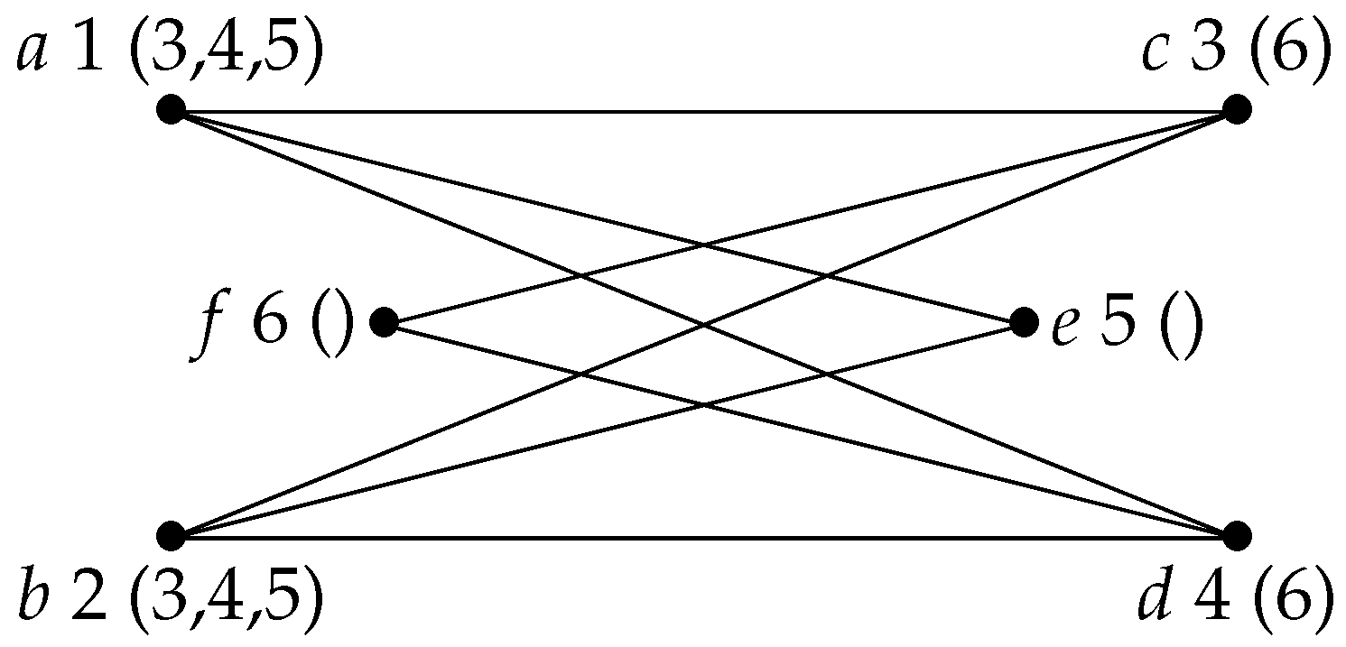
Counterexample 1.
An execution of the algorithm DCL-MLS-CliqueTree on the graph H shown in Figure 1 and the labeling structure computing ordering is shown in Figure 2. For each vertex x, the number and the final label of x are indicated. At the beginning of Iteration 4, -- and , with according to labeling structure . At Iteration 4, vertex d is chosen, and as --, the execution increases the current clique instead of starting new clique .
4. Clique Tree of the Complement Graph
The algorithm MLS can be used to compute a PEO of the complement graph [11]. We will show that it can be used to compute a PMO, a clique tree and the minimal separators of the complement graph, provided that this complement graph is connected and chordal.
Definition 6.
Let be a labeling structure. is complement-reversing if for any integers i and n with and any subsets I and of , if , then .
Remark 2.
[11] For each , is complement-reversing.
Definition 7.
For any labeling structure , denotes the labeling structure obtained from by replacing the order on the labels by its dual order.
Theorem 5.
[11] Let be a complement-reversing labeling structure. Then, an ordering of a graph G is a -MLS ordering of if and only if it is a -MLS ordering of G.
Thus, if is complement-reversing, then replacing “maximal” by “minimal” in the algorithm MLS results in an algorithm that, with G and as input, computes a -MLS ordering of G and therefore a -MLS ordering of , which is a PEO of if it is chordal. However, it is not correct to replace in the algorithm moplex-MLS or MLS-CliqueTree condition “if possible strictly greater than --” by “if possible strictly smaller than --” since in the case . With , we have , i.e., -- at iteration i (as x is adjacent to in H, it is not adjacent to in G, and therefore, its label is not increased during iteration ). We will show that -- is a necessary and sufficient condition for starting a new clique in H, whether the labeling structure is DCL or not.
Thus, the algorithm complement-DCL-MLS-CliqueTree (Algorithm 8) detects new cliques on the complement of the input graph by a condition on labels whether the labeling structure is DCL or not.
| Algorithm 8: complement-DCL-MLS-CliqueTree. |
 |
Note that as by condition, IC labels can only increase, -- is necessarily minimal.
Theorem 6.
The algorithm complement-DCL-MLS-CliqueTree is correct.
An ordering computed by the algorithm complement-DCL-MLS-CliqueTree is a -MLS ordering of G, and therefore, by Theorem 5 a -MLS ordering of H, which is a PEO of H. To prove Theorem 6, we will use the following Lemma.
Lemma 4.
In an execution of complement-DCL-MLS-CliqueTree, for each i in and each y in V such that , at the beginning of iteration i, the following propositions are equivalent:
- (1)
- ,
- (2)
- --,
- (3)
- .
Proof.
(1) ⇒ (2): We suppose that . Then, , and therefore, by Lemma 1, --. Moreover, -- since and -- are the labels of y and , respectively, at the beginning of iteration . Hence, --.
(2) ⇒ (3): We suppose that --. Then, the label of y is not increased during iteration (otherwise, it would have been strictly smaller than the label of at the beginning of iteration ). It follows that y is not adjacent to in G and therefore is adjacent to in H. As α is a PEO of H, . Moreover, , since otherwise, , and therefore, by Lemma 1, --. Hence, .
(3) ⇒ (1) is evident. ☐
Proof.
(of Theorem 6) Let be the ordering computed by an execution of complement-DCL-MLS-CliqueTree on input G and , and let . Let us show that it is a PMO of H, i.e., a MCComp PEO of H by Characterization 3. As α is an MLS ordering of H, it is a PEO of H. Let . We suppose that is not a maximal clique of H. Let us show that it is equal to . As is not a maximal clique of H, there is a vertex y, such that and , and therefore, by Lemma 4, -- at the beginning of iteration i in this execution. It follows by the condition on the choice of x that -- and, therefore, by Lemma 4 that .
It remains to show that condition -- correctly detects new cliques. It is evident at iteration n. For each iteration i with , it immediately follows from Lemma 4, as the condition to start a new clique is , i.e., by Invariant 2 (e). ☐
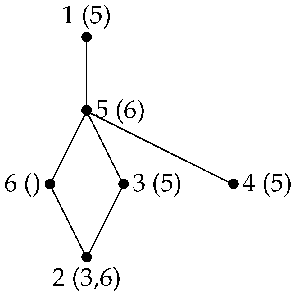
Example 3.
Let G be the complement graph of the graph H shown in Figure 1. An execution of the algorithm complement-DCL-MLS-CliqueTree on G and labeling structure computing ordering is shown in Figure 3. For each vertex x, the number and the final label of x are indicated. At the beginning of Iteration 4, and , with according to labeling structure and --; vertex d is chosen, and new clique is started at Iteration 4 as desired. Clique K is correctly started at Iteration 2 since -- and .
The algorithm complement-DCL-MLS-CliqueTree does not run in time, since computing S (in order to compute the maximal cliques and minimal separators of ) and k in StartClique (in order to compute the edges of the clique tree) globally, takes time, where is the number of edges of . However, the algorithm complement-DCL-MLS-generators (Algorithm 9) computes a PMO α and the generators of the maximal cliques and minimal separators w.r.t. α of in time.
| Algorithm 9: complement-DCL-MLS-generators. |
 |
Theorem 7.
The algorithm complement-DCL-MLS-generators is correct, and if the input labeling structure is with , then it runs in linear time.
Proof.
Correctness follows from the correctness of complement-DCL-MLS-CliqueTree.
We suppose that the input labeling structure is with . As the order on the labels is total, it is sufficient to choose a vertex x with the minimal label at each iteration. The linear time complexity of -MLS also holds for -MLS. Hence, it is sufficient to check that condition -- can be evaluated in time. This is obviously the case if . This is also the case if , since is of length at most . ☐
5. Extended Results
5.1. Clique Tree of a Minimal Triangulation
The algorithm MLSM computes an MEO and the associated minimal triangulation of the input graph G. It computes an MMO of G if the order on labels is total [12]. It can be modified into the algorithm moplex-MLSM computing an MMO of G whether the order on labels is total or not, which can be extended to the algorithms MLSM-CliqueTree and DCL-MLSM-CliqueTree computing an MMO, the associated minimal triangulation H of G, a clique tree and the minimal separators of H. Below are the algorithms moplex-MLSM and DCL-MLSM-CliqueTree (Algorithms 10 and 11).
| Algorithm 10: moplex-MLSM. |
 |
Theorem 8.
The algorithm moplex-MLSM computes an MMO and the associated minimal triangulation of the input graph.
To prove Theorem 8, we will use the following lemmas.
Lemma 5.
[8] A moplex of a minimal triangulation of G is a moplex of G.
Lemma 6.
If α is an MEO of G and a PMO of , then it is an MMO of G.
Proof.
Let . We prove this by induction on the size k of the perfect moplex partition associated with α in H. If , then H is a clique, so G is a clique, as well, since H is a minimal triangulation of G, and we are done. We assume that the property holds for a perfect moplex partition of size . Let be the perfect moplex partition associated with α in H. As is a moplex of H, by Lemma 5, it is a moplex of G. Let be the graph obtained from G by saturating and removing , and let be the restriction of α to .
As α is an MEO of G, is an MEO of and as , is a PMO of . Hence, by the induction hypothesis, is an MMO of , and therefore, α is an MMO of G. ☐
Note that the fact that α is a PMO of does not imply that it is an MMO of G. For instance, if G is a non-clique graph with a universal vertex, then any ordering α of G such that is universal is a PMO of (since is a clique), but not an MMO of G (since it is not an MEO of G).
Proof.
(of Theorem 8) Let α be the ordering and H be the graph computed by an execution of moplex-MLSM on input graph G. As this execution is also an execution of MLSM, α is an MEO of G and . As moreover at each iteration, the labels are increased exactly in the same way as in an execution of moplex-MLS on H, α is a PMO of H and, therefore, an MMO of G by Lemma 6. ☐
| Algorithm 11: DCL-MLSM-CliqueTree. |
 |
The correctness of the algorithm DCL-MLSM-CliqueTree immediately follows from the correctness of the algorithms moplex-MLSM and DCL-MLS-CliqueTree.
5.2. Atom Tree and Clique Minimal Separators
An atom tree of a connected graph G can be computed from a clique tree of a minimal triangulation of G as described in the following theorem.
Theorem 9.
[20] Let G be a connected graph; let H be a minimal triangulation of G; let be a clique tree of H; and let be the forest obtained from T by removing all edges such that is a clique in G; let be the tree obtained from T by merging the nodes of each tree of into one node; then, is an atom tree of G, and for each edge of T such that is a clique in G, , where A and are the atoms of G containing K and , respectively.
Thus, the algorithm DCL-MLSM-CliqueTree can be modified into the algorithm DCL-MLSM-AtomTree computing an atom tree and the clique minimal separators of the input graph G: in case a new clique is started, a new atom is started only if S is a clique in G; otherwise, the atom containing is increased. Note that the atoms are not built one after another, since an atom different from may be increased if a new clique is started and S is not a clique in G. Variable q contains the index of the current atom. The algorithm DCL-MLSM-AtomTree (Algorithm 12) generalizes the algorithm MCSM-atom-tree from [20], while correcting an error in this algorithm (a confusion between variables q and s).
InitAT // Initialize the Atom Tree
; ; ; ; ; ;
StartAtom // Start a new Atom
;
; ;
IncreaseAtom // Increase the current Atom
; ;
DefineAT // Define the Atom Tree
;
| Algorithm 12: DCL-MLSM-AtomTree. |
 |
The correctness of the algorithm DCL-MLSM-AtomTree follows from Theorem 9, Characterization 2 and from the correctness of the algorithm DCL-MLSM-CliqueTree.
5.3. MLS on a Non-Chordal Graph
A MLS ordering of a non-chordal graph G is not necessarily an MEO of G. It was shown in [8] that LexBFS ends on a moplex, i.e., if α is a LexBFS ordering of a non-clique graph G, then there is a moplex of G such that . As the restriction of α to is a LexBFS ordering of , it follows that α is compatible with a simple moplex partition of G. However, if G is not chordal, then α is not necessarily a PMO of G, and it is not necessarily an MMO of G and not even an MEO of G.
Example 4.
Let G be the graph shown in Figure 4, and let . α is a LexBFS ordering of G (the final labels are indicated). α is compatible with the simple moplex partition . However, α is not an MEO of G since the graph (shown in the figure with dashed fill edges) is not a minimal triangulation of G.
The work from [8] also showed that if α is a LexBFS ordering of a graph G, then the minimal separators included in are totally ordered by inclusion and that α consecutively numbers the vertices of each connected component of and its neighborhood. More accurately, there is an order on the connected component of , such that for each i in ; (the minimal separators included in are the sets ), and α is compatible with the ordered partition , where is the moplex containing . Xu et al. [14] showed that LexDFS also ends on a moplex of the input graph G (and therefore, a LexDFS ordering is compatible with a simple moplex partition of G), but they left open the question whether LexDFS orderings also have the properties on minimal separators and connected components. The following counterexample shows that these properties of LexBFS do not extend to LexDFS.
Counterexample 2.
Let G be the graph shown in Figure 5, and let . α is a LexDFS ordering of G (the final labels are indicated). The minimal separators included in are and and are incomparable for inclusion. If the property on connected components was true, would be the component numbered last by α, i.e., , but the vertices of (7, 6 and 2) are not numbered consecutively by α. If G is the graph shown in Figure 6 with , even the restriction of α to is not compatible with a sequence of the connected components of .
It is shown in [12] that for each labeling structure with a total order on labels and each -MLS ordering α of a graph G, is an OCF-vertex of G, i.e., satisfies the property: for each pair of non-adjacent vertices in , there is a connected component C of such that . However, the definition of a labeling structure given in [12] is less general than the definition given in this paper, as IC is replaced by conditions (p1): and (p2): : (p1) and (p2) imply IC and IC implies (p1), but does not imply (p2). It turns out that the property of being an OCF-vertex does not extend to a labeling structure defined with IC instead of (p1) and (p2) (a counterexample can be built with some effort). It is the only result from [12] that does not extend to a labeling structure defined with IC.
6. Conclusions
In this paper, we explain how a clique tree of a chordal graph H can be computed from an arbitrary PEO of H, from a PMO of H and from a modification of the algorithm MLS. We show that a PMO allows one to build the cliques of a clique tree one after another. We characterize labeling structures for which it is possible to detect the beginning of a new clique using the labels and show that each labeling structure can detect this with labels when building a clique tree of the complement graph.
Some results concerning algorithm MLS in Section 3 and MLSM in Section 5 are generalizations of the results already known for MCS, LexBFS or MCS-M. The proofs in this paper largely use Inclusion Condition (IC) (through Lemma 1) and make it clear that IC is fundamental for the properties of the computed orderings. We believe that many results proven for some particular instances of MLS or MLSM can be proven in a more general way for MLS or MLSM using IC. This has already been done in [10,12,20]. We leave open the question of which other results could be generalized using IC and which applications could follow from these generalizations.
Acknowledgments
We thank the reviewers for their helpfull comments and suggestions.
Author Contributions
Anne Berry and Geneviève Simonet both provided the contents and wrote the paper.
Conflicts of Interest
The authors declare no conflict of interest.
References
- Dirac, G.A. On rigid circuit graphs. Abh. Math. Sem. Univ. Hamburg 1961, 25, 71–76. [Google Scholar] [CrossRef]
- Fulkerson, D.R.; Gross, O.A. Incidence matrixes and interval graphs. Pac. J. Math. 1965, 15, 835–855. [Google Scholar] [CrossRef]
- Gavril, F. The Intersection Graphs of Subtrees in Trees Are Exactly the Chordal Graphs. Combin. Theory Ser. B 1974, 16, 47–56. [Google Scholar] [CrossRef]
- Blair, J.R.S.; Peyton, B.W. An introduction to chordal graphs and clique trees. Graph Theory Sparse Matrix Comput. 1993, 84, 1–29. [Google Scholar]
- Tarjan, R.E.; Yannakakis, M. Simple linear-time algorithms to test chordality of graphs, test acyclicity of hypergraphs, and selectively reduce acyclic hypergraphs. SIAM J. Comput. 1984, 13, 566–579. [Google Scholar] [CrossRef]
- Rose, D.J.; Tarjan, R.E.; Lueker, G.S. Algorithmic aspects of vertex elimination on graphs. SIAM J. Comput. 1976, 5, 266–283. [Google Scholar] [CrossRef]
- Kumar, P.S.; Madhavan, C.E.V. Minimal vertex separators of chordal graphs. Discret. Appl. Math. 1998, 89, 155–168. [Google Scholar] [CrossRef]
- Berry, A.; Bordat, J.P. Separability generalizes Dirac’s theorem. Discret. Appl. Math. 1998, 84, 43–53. [Google Scholar] [CrossRef]
- Corneil, D.G.; Krueger, R. A unified view of graph searching. SIAM J. Discret. Math. 2008, 22, 1259–1276. [Google Scholar] [CrossRef]
- Berry, A.; Krueger, R.; Simonet, G. Maximal Label Search Algorithms to Compute Perfect and Minimal Elimination Orderings. SIAM J. Discret. Math. 2009, 23, 428–446. [Google Scholar] [CrossRef]
- Krueger, R.; Simonet, G.; Berry, A. A General Label Search to investigate classical graph search algorithms. Discret. Appl. Math. 2011, 159, 128–142. [Google Scholar] [CrossRef] [Green Version]
- Berry, A.; Blair, J.R.S.; Bordat, J.-P.; Simonet, G. Graph extremities defined by search algorithms. Algorithms 2010, 3, 100–124. [Google Scholar] [CrossRef] [Green Version]
- Berry, A.; Pogorelcnik, R. A simple algorithm to generate the minimal separators and the maximal cliques of a chordal graph. Inform. Process. Lett. 2011, 111, 508–511. [Google Scholar] [CrossRef] [Green Version]
- Xu, S.-J.; Li, X.; Liang, R. Moplex orderings generated by the LexDFS algorithm. Discret. Appl. Math. 2013, 161, 2189–2195. [Google Scholar] [CrossRef]
- Berry, A.; Pogorelcnik, R.; Simonet, G. An introduction to clique minimal separator decomposition. Algorithms 2010, 3, 197–215. [Google Scholar] [CrossRef] [Green Version]
- Berry, A.; Wagler, A. Triangulation and clique separator decomposition of claw-free graphs. In Proceedings of the WG 2012, Jerusalem, Israel, 26–28 June 2012; pp. 7–21.
- Brandstädt, A.; Hoàng, C.T. On clique separators, nearly chordal graphs, and the Maximum Weight Stable Set Problem. Theoret. Comput. Sci. 2007, 389, 295–306. [Google Scholar] [CrossRef]
- Leimer, H.-G. Optimal decomposition by clique separators. Discret. Math. 1993, 113, 99–123. [Google Scholar] [CrossRef]
- Tarjan, R.E. Decomposition by clique separators. Discret. Math. 1985, 55, 221–232. [Google Scholar] [CrossRef]
- Berry, A.; Pogorelcnik, R.; Simonet, G. Organizing the atoms of the clique separator decomposition into an atom tree. Discret. Appl. Math. Math. 2014, 177, 1–13. [Google Scholar] [CrossRef] [Green Version]
- Berry, A.; Blair, J.R.S.; Heggernes, P.; Peyton, B.W. Maximum cardinality search for computing minimal triangulations of graphs. Algorithmica 2004, 39, 287–298. [Google Scholar] [CrossRef]
- Brandstädt, A.; Le, V.B.; Spinrad, J.P. Graph Classes: A Survey; Monographs on Discrete Mathematics and Applications; Society for Industrial and Applied Mathematics: Philadelphia, PA, USA, 1999; Volume 3. [Google Scholar]
- Golumbic, M.C. Algorithmic Graph Theory and Perfect Graphs; Academic Press: New York, NY, USA, 1980. [Google Scholar]
- Berry, A.; Bordat, J.P. Moplex elimination orderings. Electron. Notes Discret. Math. 2001, 8, 6–9. [Google Scholar] [CrossRef]
- Rose, D.J. Triangulated graphs and the elimination process. J. Math. Anal. Appl. 1970, 32, 597–609. [Google Scholar] [CrossRef]
- Spinrad, J.P. Efficient Graph Representations; Fields Institute Monographs, American Mathematical Society: Presidence, RI, USA, 2003. [Google Scholar]
Figure 1.
A chordal graph H.
Figure 2.
LexDFS labels do not detect new maximal cliques.
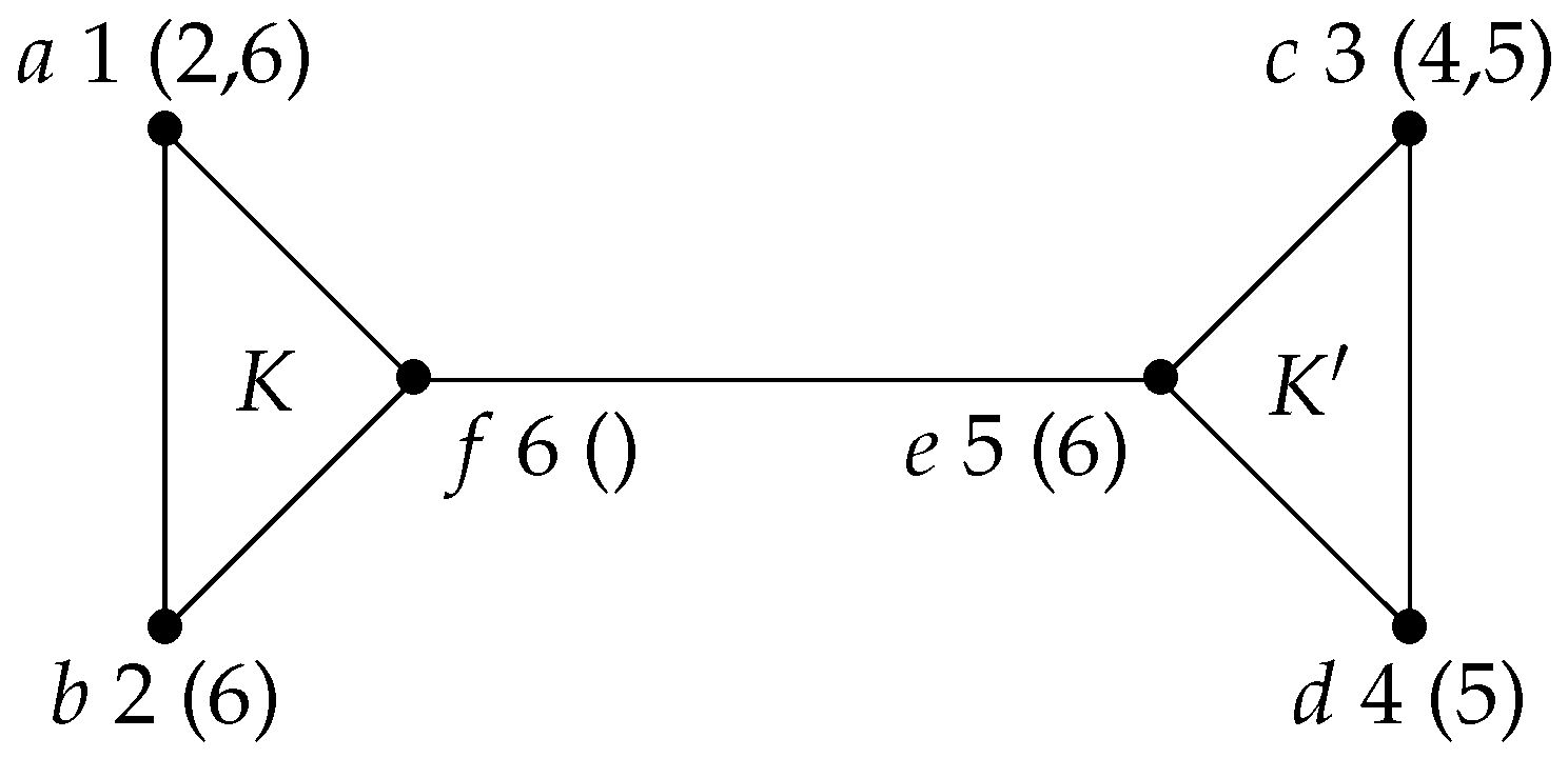
Figure 3.
Lexicographic Depth-First Search (LexDFS) labels detect new cliques on the complement.

Figure 4.
Lexicographic Breadth-First Search (LexBFS) on a non-chordal graph computes an ordering that is compatible with a simple moplex partition, but not with an MEO.
Figure 4.
Lexicographic Breadth-First Search (LexBFS) on a non-chordal graph computes an ordering that is compatible with a simple moplex partition, but not with an MEO.
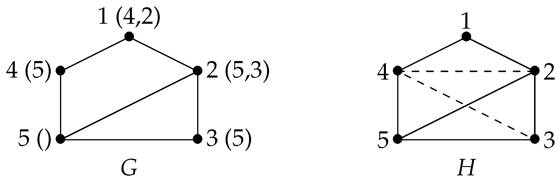
Figure 5.
With LexDFS, the minimal separators included in are not totally ordered by inclusion.
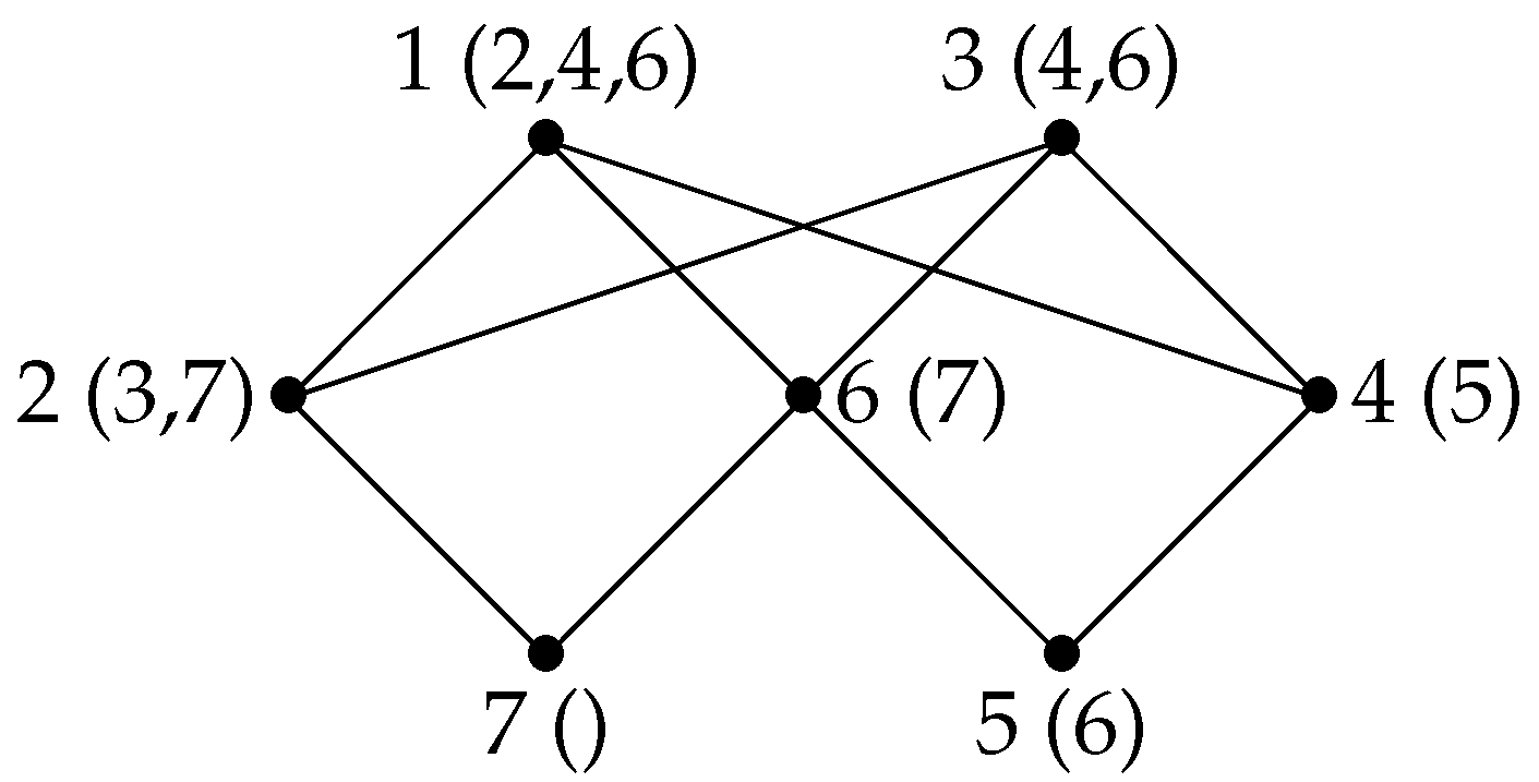
Figure 6.
LexDFS does not number the connected components of one after another.

© 2017 by the authors. Licensee MDPI, Basel, Switzerland. This article is an open access article distributed under the terms and conditions of the Creative Commons Attribution (CC BY) license ( http://creativecommons.org/licenses/by/4.0/).
Share and Cite
MDPI and ACS Style
Berry, A.; Simonet, G. Computing a Clique Tree with the Algorithm Maximal Label Search. Algorithms 2017, 10, 20. https://doi.org/10.3390/a10010020
AMA Style
Berry A, Simonet G. Computing a Clique Tree with the Algorithm Maximal Label Search. Algorithms. 2017; 10(1):20. https://doi.org/10.3390/a10010020
Chicago/Turabian StyleBerry, Anne, and Geneviève Simonet. 2017. "Computing a Clique Tree with the Algorithm Maximal Label Search" Algorithms 10, no. 1: 20. https://doi.org/10.3390/a10010020
Note that from the first issue of 2016, this journal uses article numbers instead of page numbers. See further details here.