
Efficient Algorithms for the Maximum Sum Problems

1
Algorithm Research Institute, Christchurch 8053, New Zealand
2
Computer Science and Software Engineering, University of Canterbury, Christchurch 8140, New Zealand
*
Author to whom correspondence should be addressed.
Algorithms 2017, 10(1), 5; https://doi.org/10.3390/a10010005
Submission received: 9 August 2016
/
Revised: 2 December 2016
/
Accepted: 26 December 2016
/
Published: 4 January 2017
Abstract
:We present efficient sequential and parallel algorithms for the maximum sum (MS) problem, which is to maximize the sum of some shape in the data array. We deal with two MS problems; the maximum subarray (MSA) problem and the maximum convex sum (MCS) problem. In the MSA problem, we find a rectangular part within the given data array that maximizes the sum in it. The MCS problem is to find a convex shape rather than a rectangular shape that maximizes the sum. Thus, MCS is a generalization of MSA. For the MSA problem, time parallel algorithms are already known on an 2D array of processors. We improve the communication steps from to n, which is optimal. For the MCS problem, we achieve the asymptotic time bound of on an 2D array of processors. We provide rigorous proofs for the correctness of our parallel algorithm based on Hoare logic and also provide some experimental results of our algorithm that are gathered from the Blue Gene/P super computer. Furthermore, we briefly describe how to compute the actual shape of the maximum convex sum.
1. Introduction
We face a challenge to process a big amount of data in the age of information explosion and big data [1]. As the end of Moore’s law comes in sight, however, the extra computing power is unlikely obtained from a single processor computer [2]. Parallel computing is obviously a direction to faster computation. However, efficient utilization of the parallel architecture is not an effortless task. New algorithms often need to be designed for specific problems on specific hardware.
In this paper, we investigate the maximum subarray (MSA) problem and the maximum convex sum (MCS) problem, the latter being a generalization of the former. We design efficient parallel algorithms for both problems and an improved sequential algorithm for the MCS problem.
The MSA problem is to find a rectangular subarray in the given two-dimensional (2D) data array that maximizes the sum in it. This problem has wide applications from image processing to data mining. An example application from image processing is to find the most distinct spot, such as brightest or darkest, in the given image. If all pixel values are non-negative, solving the MSA problem will return the trivial solution of the whole array. Thus, we normalize the input image (e.g., by subtracting the mean value), such that the relatively brighter spots will have positive sums, while the relatively darker spots will have negative sums. Then, solving the MSA problem on the normalized image can give us the brightest spot in the image. In data mining, suppose we spread the sales amounts of some product on a two-dimensional array classified by customer ages and annual income. Then, after normalizing the data, the maximum subarray corresponds to the most promising customer range.
We now consider the MCS problem that maximizes the sum in a convex shape. The definition of the word “convex” is not exactly the same as that in geometry. We define the convex shape as the joining of a W-shape and an N-shape, where W stands for widening and N for narrowing. We call this shape the -convex shape or -shape for short. In W, the top boundary goes up or stays horizontal when scanned from left to right, and the bottom boundary goes down or stays horizontal. Fukuda et al. defines a more general rectilinear shape [3], but for simplicity, we only consider the -shape. The paper is mainly devoted to computing the maximum sum, and one section is devoted to the computation of the explicit convex shape that provides the sum.
We give an example to illustrate how solving the MCS problem can provide a much more accurate data analysis compared to solving the MSA problem. We compared the size of the hole in the ozone layer over Antarctica between 2006 and 2011 by solving both the MSA problem and the MCS problem on the normalized input images (Figure 1a,d, respectively) of the Antarctic region. Figure 1b,e is from solving the MSA problem on the input images, while Figure 1c,f is from solving the MCS problem on the same set of input images. Solving the MCS problem clearly provides a much more accurate representation of the ozone hole. The numeric value returned by the MCS is also 22%~24% greater than that by the MSA on both occasions. Intuitively similar gains from the -shape compared to the rectangular shape can be foreseen for other types of data analysis.
In this paper, we assume that the input data array is an square two-dimensional (2D) array. It is a straightforward exercise to extend the contents of this paper to rectangular 2D input data arrays.
The typical algorithm for the MSA problem by Bentley [4] takes time on a sequential computer. This has been improved to a slightly sub-cubic time bound by Tamaki and Tokuyama [5] and also Takaoka [6]. For the MCS problem, an algorithm with time is given by Fukuda et al. [3], and an algorithm with a sub-cubic time bound is not known.
Takaoka discussed a parallel implementation to solve the MSA problem on a PRAM [6]. Bae and Takaoka implemented a range of parallel algorithms for the MSA problem on an 2D mesh array architecture based on the row-wise or column-wise prefix sum [7,8,9]. A parallel algorithm for the MSA problem was also implemented on the BSP/CGMarchitecture, which has more local memory and communication capabilities with remote processors [10].
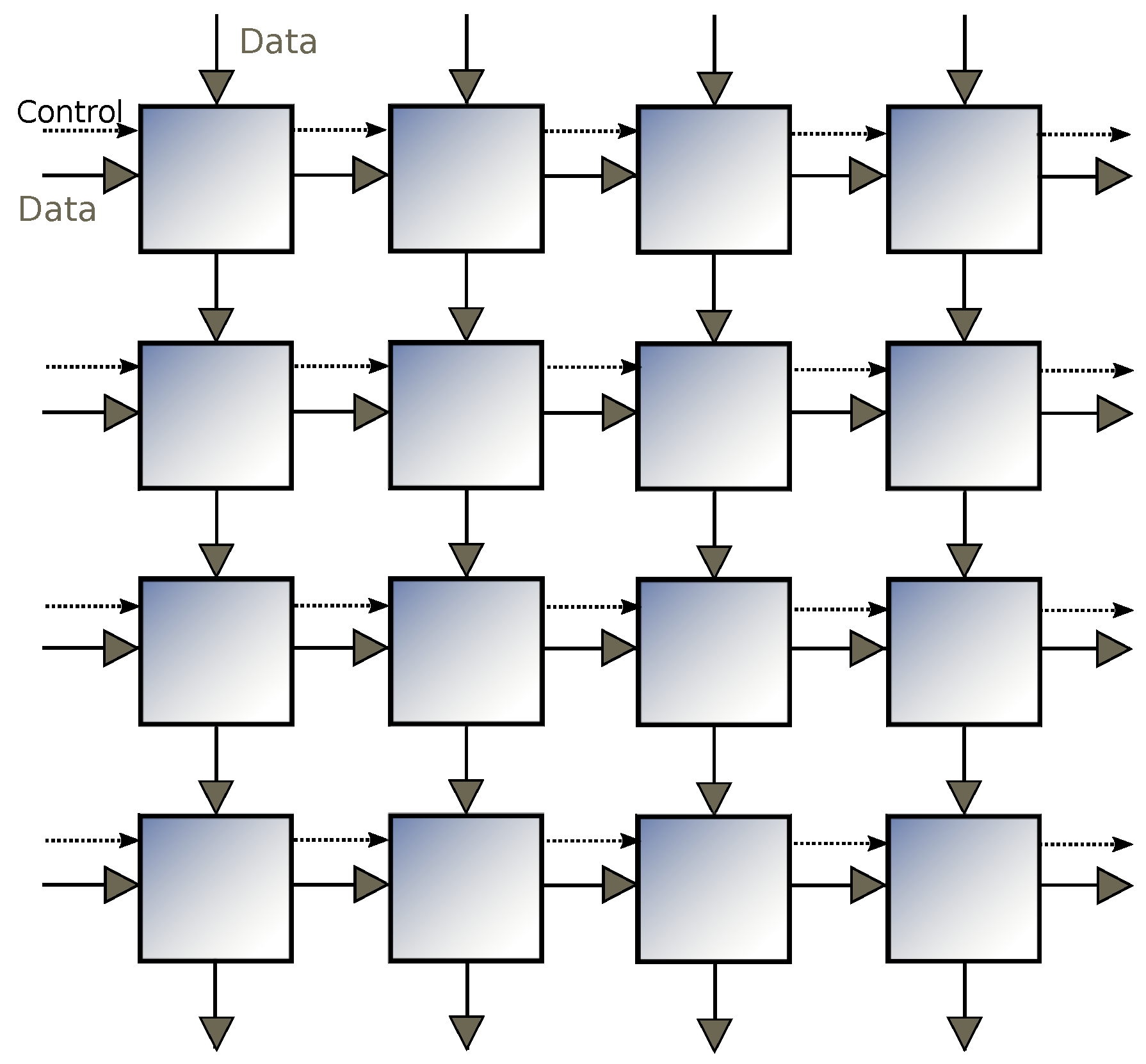
In this paper, we implement algorithms for the MSA and MCS problems based on the column-wise prefix sum on the 2D mesh architecture, as shown by Figure 2. This architecture is also known as a systolic array, where each processing unit has a constant number of registers and is permitted to only communicate with directly-connected neighbours. This seemingly inflexible architecture is well suited to be implemented on ASICs or FPGAs.
Our most efficient parallel algorithms complete the computation in communication steps for the MSA problem and communication steps for the MCS problem, respectively. In each step, all cells execute a constant number of statements in parallel. Thus, our algorithms are cost optimal with respect to the cubic time sequential algorithms [3,4].
We give a formal proof for the parallel algorithm for computing the maximum W (a part of computing the MCS problem). The proof is based on the space-time invariants defined on the architecture.
In a 2D array architecture, some processors to the right are sitting idle in the early stage of computation waiting for inputs to arrive. This is because the data only flows from left to right and from up to down (Figure 2). If appropriate, we attempt to maximize the throughput by extending data flows to operate in four directions. This technique reduces the number of communication steps by a constant factor.
Algorithms are given by pseudocode.
2. Parallel Algorithms for the MSA Problem
In this section, we improve parallel algorithms for the MSA problem on a mesh array and achieve the optimal n communication steps. Furthermore, we show how the programming techniques in this section lead to efficient parallel algorithms for the MCS problem in the later sections.
2.1. Sequential Algorithm
The computation in Algorithm 1 [8] proceeds with the strip of the array from position k to position i. See Figure 3. The variable is the sum of array elements in the j-th column from position k to position i in array a. The variable , called a prefix-sum, is the sum of the strip from Position 1 to position j. Within this strip, variable j sweeps to compute by adding to . Then, the prefix sum of this strip from Position 1 to position j is computed by adding to . The variable is the minimum prefix sum of this strip from Position 1 to position j. If the current is smaller than , is replaced by it. is the maximum sum in this strip so far found from Position 1 to position j. It is computed by taking the maximum of and , expressed by in the figure. After the computation for this strip is over, the global solution, S, is updated by . This computation is done for all possible i and k, taking time.
| Algorithm 1 MSA: sequential. |
|
2.2. Parallel Algorithm 1
Algorithm 2 is a parallel adaptation of Algorithm 1. The following program is executed by a processing unit at the grid point, which we refer to as . Each is aware of its position . Data flow is from left to right and from top to bottom. The control signals are fired at the left border and propagate right. When the signal arrives at , it accumulates the column sum “”, the sum “” and updates the minimum prefix sum “”, etc. Figure 4 illustrates the information available to at step k. At step , will have computed the maximum sum. We assume that all corresponding instructions in all cells are executed at the same time, that is they are synchronized. We will later make some comments on asynchronous computation.
| Algorithm 2 MSA Parallel 1. |
Initialization
|
2.3. Parallel Algorithm 2
This algorithm (Algorithm 3) does communication bi-directionally in a horizontal way. For simplicity, we assume n is even. The mesh is divided into two halves, left and right. The left half operates in the same way as Algorithm 2. The right half operates in a mirror image, that is control signals go from right to left initiated at the right border. All other data also flow from right to left. At the centre, that is at , performs “”, which adds the two values that are the sums of strip regions in the left and right whose heights are equal and, thus, can be added to form a possible solution crossing over the centre. At the end of the k-th iteration, all properties in Algorithm 2 hold on the left half, and the properties in the mirror image hold on the right half. In addition, we have that is the value of the maximum subarray that lies above or that is touching the i-th row and crosses over the centre line.
| Algorithm 3 MSA Parallel 2. |
Initialization
|
The strip processes is in the left half, and that in the right half is . Thus, the cells and processes the strips of the same height in the left half and the right half. Communication steps are measured by the distance from to or, equivalently, from to , which is . By adding the finalization step, we have for the total communication steps.
2.4. Parallel Algorithm 3
In Algorithm 4, data flow in four directions. The array is divided into two halves; left and right, as in the previous section. Column sums c and prefix sums s accumulate downwards as before, whereas column sums d and prefix sums t accumulate upwards. See Figure 5.
| Algorithm 4 MSA Parallel 3: initialization. |
|
The structure of Algorithm 4 reveals that at the end of the k-th iteration, is the sum of and is the sum of . The height of each subarray is . Since the widths of those two areas are the same, we can have the prefix sum that covers , the height of which is . That is, spending k steps, we can achieve twice as much height as that in Algorithm 3.
The solution array is calculated as before, but the result is sent into three directions; up, down and right in the left half and up, down and left in the right half. We have the property that is the maximum sum in subarray in the left half. Substituting , and yields the subarray . Similarly, is the maximum sum in the subarray . For simplicity, we deal with the maximum subarray whose height is an even number. For a general case, see the note at the end of this section.
The computation proceeds with steps by k and the last step of comparing the results from and , resulting in steps in total.
Note that we described the algorithm for the solution whose height is an even number. This fact comes from the assignment statement “” where the heights of subarrays whose sums are s and t are equal. To accommodate a height of an odd number, we can use the value of t one step before, whose height is one shorter. To accommodate such odd heights, we need to almost double the size of the program by increasing the number of variables.
3. Review of Sequential Algorithm for the MCS Problem
We start from describing a sequential algorithm for W based on column sums, given by Fukuda et al. [3]. We call the rightmost column of a W-shape the anchor column of W. The array portion of general array b, , is the rectangular portion whose top left corner is , and the bottom right corner is . The column is abbreviated as . In Algorithm 5, is a W-shape based on the anchor column of . The sum of this anchor column is given by .
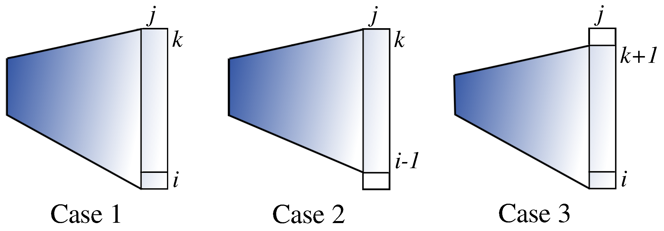
The computation proceeds with the strip of the array from row k to row i (Figure 6) based on dynamic programming. Within this strip from row k to row i, variable j sweeps to compute by adding to (Case 1 of Figure 7) or extending a W-shape downward or upward by one (Cases 2 and 3 of Figure 7, respectively). Note that the width of the strip is given by . That is, we go through from thinner to thicker strips, so that the results for thinner ones are available when needed for Cases 2 and 3. Obviously, Algorithm 5 takes time.
| Algorithm 5 Sequential algorithm for W. |
Initialization
|
After all W are computed, we compute the N-shape in array N for all anchor columns by a mirror image of the algorithm for W. Then, the finalization of the -shape is given by Algorithm 6.
| Algorithm 6 Combining W and N. |
|
Note that the W-shape and the N-shape share the same anchor column, meaning we need to subtract one . This computation is done for all possible i, j and k, taking time, resulting in time for the maximum convex sum.
4. Improved Sequential Algorithm
We can observe that Algorithm 5 not only takes time, but also requires memory. The reason for this memory requirement is that the algorithm stores maximum W and maximum N for all possible anchor columns.
We can improve the memory requirement of Algorithm 5 significantly to with a simple modification. Firstly, we observe that there is no reason to keep all maximum W and maximum N for all possible anchor columns. Instead, we can iterate over the possible anchor column sizes and compute the maximum W and N for the given anchor column size in each iteration, thereby computing the maximum for the given anchor column size in each iteration. Thus, in each iteration, we only need memory, and there is no need to store maximum W and N values from previous iterations. Note that W and N on shorter columns are available for the t-th iteration.
Algorithm 7 is the pseudocode for achieving the memory bound. The pseudocode has been simplified, since much of the details have already been provided in Section 3.
| Algorithm 7 Sequential algorithm for . |
|
We note that the reduction in the memory bound is very significant in practical terms. The difference between memory and memory, if we take image processing as an example, is the difference between being able to process a mega-pixel image entirely in memory and having to resort to paging the results in an incomparably slow execution time.
5. Parallel Algorithm for MCS
We now give a parallel algorithm that corresponds to the sequential algorithm described in Section 3. Algorithm 8 is executed by the cell at the grid point. Each is aware of its position . Data flow is from left to right and from top to down. The control signals are fired at the left border and propagate right. When the signal arrives at , it starts to accumulate the column sum and update , W and . The value of at time k is to hold the maximum W-value based on the anchor column in the j-th column from position to position i. This is illustrated in Figure 8. The value of is to hold the best W-value obtained at so far. The role of is to bring down the top value of anchor column to in time. The role of “” is to provide the value of W one step before, with being undefined.
| Algorithm 8 Parallel algorithm for W. |
Initialization
|
Note that the memory requirement for each cell in Algorithm 8 is constant. When we put W-shapes and N-shapes together, however, we need space in each cell, as we will explain later on. We assume that all corresponding instructions in all cells are executed in parallel in a synchronized manner. We later make some comments regarding how synchronization is achieved in the actual implementation of the parallel algorithm.
We prove the correctness of Algorithm 8 in the framework of Hoare logic [11] based on a restricted form of that in Owicki and Gries [12]. The latter is too general to cover our problem. We keep the minimum extension of Hoare logic to our mesh architecture.
The meaning of Hoare’s triple is that if P is true before program (segment) S, and if S halts, then Q is true after S stops. The typical loop invariant appears as that for a while-loop; “while B do S”. Here, S is a program, and B is a Boolean condition. If we can prove , we can conclude while B does , where ∼B is the negation of B. P is called the loop invariant, because P holds whenever the computer comes back to this point to evaluate the condition B. This is a time-wise invariant as the computer comes back to this point time-wise. We establish invariants in each cell. They are regarded as time-space invariants because the same conditions hold for all cells as computation proceeds. Those invariants have space indices i and j and time index k. Thus, our logical framework is a specialization of Owicki and Gries to indexed assertions.
The main assertions are given in the following. is the rectangular array portion from the top-left corner to the bottom-right corner where a candidate for the solution can be found.
At the end of the k-th iteration, the following holds in :
For and :
The above are combined to P, where:
Here, Q states that variables in each cell keep the initial values. In the following descriptions, we omit the second portion Q of the above logical formula.
We can prove that to are all true for by checking the initialization. For each to , we omit indices i and j. Using the time index k, we prove to . We use the following rules of Hoare logic. Let to be assignment statements in to in general. There can be several in each cell. We use one for simplicity. The meaning of is that the occurrence of variable in Q is replaced by . Parallel execution of to is shown by .
Parallel assignment rule:
Other programming constructs such as composition (semi-colon), if-then-else statement, etc., in sequential Hoare logic can be extended to the parallel versions. Those definitions are omitted, but the following rule for the if-then and for-loop for the sequential control structure, which controls a parallel program S from outside, is needed for our verification purpose.
Rule for if-then statement:
In our proof, corresponds to P, to B and to Q.
Rule for the for-loop:
This P represents to in our program. S is the parallel program . Each has a few local variables and assignment statements. For an arbitrary array x, we regard as a local variable for . A variable from the neighbour, , for example, is imported from the upper neighbour. Updated variables are fetched in the next cycle. The proof for each for P is given in Appendix.
Theorem 1.
Algorithm 8 is correct. The result is obtained at in steps.
Proof.
From the Hoare logic rule for the for-loop, we have at the end.
☐
We used array to compute the maximum W-shape. The value of at is ephemeral in the sense that its value changes as computation proceeds. That is, at time k holds the maximum W-shape anchored at column , and at the next step, it changes to that value of W anchored at column .
In order to combine W and N, we must memorize the maximum W and the maximum N for each anchor column. Thus, we need the three-dimensional array , as well as the array . Since in the final stage of computation, the same anchor column is added from W and N, we need to subtract the sum of the anchor column. For that purpose, the sum of anchor column is stored in . Note that the computation of N goes from right to left.
In Algorithm 9, we provide the complete algorithm that combines W and N, where is dropped, and the initialization is omitted. The computation of W and N takes steps, and takes n steps.
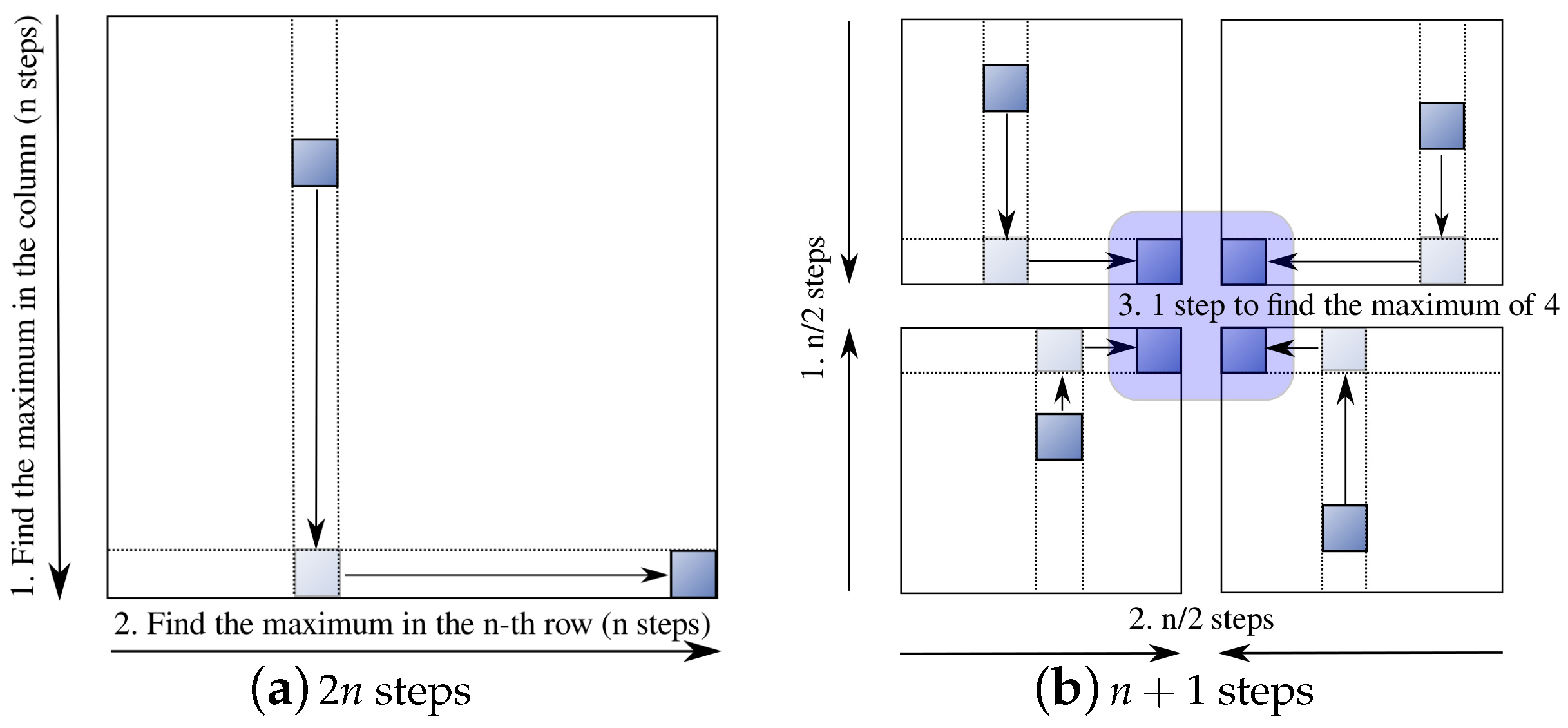
Selecting the maximum of can be done in parallel. Algorithm 10 and Figure 9a illustrate how to find the maximum in a 2D mesh in steps, where the maximum can be retrieved at the bottom right corner. If we orchestrate the bidirectional data movement in each of four quarters of the mesh (Figure 9b), so that the maximum of each quarter can meet at the centre for the final selection, it can be done in steps. Therefore, Algorithm 9 takes total of communication steps.
| Algorithm 9 Combining W and N. |
|
| Algorithm 10 Find the maximum of in steps. |
|
6. Computation of the Boundary
So far, we computed the maximum sum of the -shape. For practical purposes, we sometimes need the shape itself. This problem was solved by Thaher [13] for the sequential algorithm (Algorithm 11). We show how the idea works in our parallel situation. For simplicity, we only show the boundary computation of the W-shape. We prepare the array to memorize the direction from which the algorithm took one of Case 1, Case 2 or Case 3. This part of enhancement in Algorithm 9 is shown below.
Let array , if is on the boundary, and zero otherwise. Let denote the j-th column from position k to position i, to represent the anchor column of some W-shape. Suppose the anchor column of the maximum W-shape after Algorithm 9 is . The following sequential algorithm goes backward from guided by the data structure . The correctness of the algorithm is obvious. The time can be shown as follows.
| Algorithm 11 Computing the boundary. |
|
The time is proportional to the number of changes on indices i, j and k. The index j can be reduced at most n times. For i and k, we observe decreases whenever i or k changes, resulting in time for i and k. The time for the boundary can be absorbed in time of Algorithm 9. It will be easy to organize parallel computation of tracing back over array by the mesh architecture. For example, we can convert the array index j to a processor index j and use a one-dimensional mesh architecture as shown below (Algorithm 12).
This version has time, which provides no gain time-wise, but the space requirement on a single processor can be eased.
| Algorithm 12 Computing the boundary; j-th cell. |
|
7. Implementation
We implemented Algorithm 9 on the Blue Gene/P computer under the MPI/Parallel C program environment. There were many practical issues to be considered. We summarize just three issues here as representatives.
Firstly, we cannot assume that each cell knows its own position within the mesh array. Depending on the architecture, additional computation is required for each cell to gather this information. Within the MPI environment, we can let each know its position by the system call “MPI_Cart_coords()”.
The second issue is synchronization. We assumed the corresponding statements in all cells are executed in a synchronized manner. If we remove this assumption, that is if the execution proceeds in an asynchronous manner, the algorithm loses its correctness.
In MPI, “MPI_Send()”, “MPI_Recv()” and “MPI_Sendrecv()” functions are used to perform synchronous blocking communications [14]. As we call these functions in each step, no further mechanisms are necessary to ensure synchronization between cells as the function calls ensure that any given cell cannot progress one or more steps further than the rest. In other words, one cell may reach the end of the given step and tries to move onto the next step before others, but then, the cell must wait for the other cells to reach the same point due to the blocking nature of the MPI communication functions.
The third implementation issue is related to the number of available processors. As the number of processors is limited, for large n, we need to have what is called a coarse grain parallel computer. Suppose, for example, we are given a input array and only 16 processors are available. The input array is divided into sixteen sub-arrays, to which the sixteen processors are assigned. Let us call the sub-array for each processor its territory. Each processor simulates one step of Algorithm 8 sequentially. These simulation processes by sixteen processors are done in parallel. At the end of each simulation, the values in the registers on the right and bottom border are sent to the left and top borders of the right neighbour and the lower neighbour, respectively. The simulation of one step takes time, and steps are carried out, meaning the computing time is at the cost of processors. When , we hit the sequential complexity of . If , we have the time complexity of Algorithm 8, which is .
While resolving the third implementation issue, we must again face the second issue of synchronization. For each processor to simulate the parallel computation in its own territory in a coarse-grained implementation, we must take extra care to ensure synchronization between simulated cells within each territory. Specifically, we must double the number of variables, that is we prepare variable for every variable x. Let us associate the space/time index, with each variable. Let us call the current variable and the variable with indices different by one a neighbour variable. For example, in the right-hand side of the assignment statement is a time-wise neighbour, and that at the left-hand side is a current variable. Furthermore, in the right-hand side is a neighbour variable space-wise and time-wise, and so on. If x is a current variable, change it to . If it is a variable of a neighbour, keep it as it is. Let us call the modified program . Now, we define “update” to be the set of assignment statements of the form .
Example 1.
Let P be a one-dimensional mesh program given by Algorithm 13, which shifts array x by one place. Let us suppose and are already given.
In Algorithm 13, is the current variable, and is a neighbour variable space-wise and time-wise. An asynchronous computer can make all values zero. For the intended outcome, we perform , given by Algorithm 14, which includes “synchronize” and “update”.
| Algorithm 13 Program P. |
|
| Algorithm 14 Program . |
|
For our mesh algorithm, Algorithm 8, omitting the initialization part, we make the program of the form that is given by Algorithm 15.
| Algorithm 15 Synchronization for coarse grain. |
|
Algorithm 9 was executed on Blue Gene/P with up to 1024 cores. For the software side, the programming environment of MPI and the parallel C compiler, mpixlc, were used with Optimization Level 5. The results are shown in Table 1. Arrays of size containing random integers were tested. The times for generating uniformly-distributed random numbers, as well as loading the data onto each processor were not included in the time measurement. On Blue Gene/P, the mesh architecture can be configured into a 2D mesh or 3D mesh. The time taken to configure the mesh into a 2D mesh array for our algorithm was included in the time measurement. As we can see from the table, for small n, the configuration time dominates, and increasing the number of processors does not result in a decrease in the execution time. As the size of the input array increases, however, we can see noticeable improvements in the execution times with a larger number of processors.
Note that we were unable to execute the program under certain configurations as shown by `x’ in Table 1. This was due to memory requirements. With large n and small p, each processor must simulate a very large territory. With each cell in the territory requiring memory to store the maximal values of W and N, the memory requirements can become prohibitive. This highlights the fact that parallelization is required not only to reduce the execution time, but also to handle larger input data.
8. Lower Bound
Algorithm 8 for W is not very efficient, as cells to the right are idling at the early stage. Suppose we are given an input array with the value a in the top-left cell and b in the bottom-right cell, while all other value are . Obviously the solution is a if , and b otherwise. The values a and b need to meet somewhere. It is easy to see that the earliest possibility is at time . Our algorithm for W takes steps, meaning there is still a gap of n steps with the lower bound. This is a sharp contrast with the mesh algorithm for MSA (Algorithm 4) that completes in steps. The role of Algorithm 8 is to establish an time for the MCS problem on the mesh architecture.
9. Concluding Remarks
We gave an time parallel algorithm for solving the MSA and MCS problem with processors and a formal proof for the algorithm to compute the W-shape, a part of the MCS problem. The formal proof for the N-shape can be given in a similar way. The formal proof not only ensures correctness, but also clarifies what is actually going on inside the algorithm.
The formal proof was simplified by assuming synchronization. The asynchronous version with (synchronize, update) in Section 7 would require about twice as much complexity for verification, since we double the number of variables. Once the correctness of the synchronized version is established, that of the asynchronous version will be acceptable without further verification.
It is open whether there is a mesh algorithm for the MCS problem with the memory requirement in each cell. Mesh algorithms are inherently easy to implement on an FPGA and, thus, can be considered for practical applications.
multiple
Appendix A. Proof for Invariants
In the following, is the sum of array portion . We assume .
Proof.
For : At the beginning of the k-th iteration, for , equivalently for . performs “” for . Thus, we have for . ☐
Proof.
For : At time , . “” is performed for and in parallel. Thus, holds. ☐
Proof.
For : At time , . At time k, “” is performed for and in parallel. Thus, , and holds. ☐
Proof.
For : At time , is the maximum of W-shapes anchored at column . By adding the sum of column , is made. is the maximum of the W-shape anchored at column . By adding , is made. is at time , which is the maximum of W-shapes anchored at column . By adding , is made. Since the maximum of the W-shape based on column is chosen from only those three possibilities, is correctly computed. ☐
Proof.
For : After , the value of changes from at to . Thus, holds. ☐
Proof.
For : The scopes for the four candidates are given below.
- at :
- at :
- at :
- at k is anchored at column with
There are only four candidates for from those four scopes. Thus, holds.
Acknowledgments
This research was supported by the EU/NZ Joint Project, Optimization and its Applications in Learning and Industry (OptALI). The experiments were conducted utilising high performance computing resources from the New Zealand eScience Infrastructure (NeSI), especially the High Performance Computing unit at the University of Canterbury (UCHPC). [NeSI-UCHPC]URL https://www.nesi.org.nz or http://www.hpc.canterbury.ac.nz.
Author Contributions
All authors contributed to the design of algorithms; T.S. provided the codes; T.S. and S.E.B. designed and performed the experiments; T.T. provided the formal proofs; S.E.B provided the figures; T.T. wrote more of the initial draft, and all authors contributed to the finalization of the paper
Conflicts of Interest
The authors declare no conflict of interest.
References
- Bell, G. Tony hey and alex szalay: Beyond the data deluge. Science 2009, 323, 1297–1298. [Google Scholar] [CrossRef] [PubMed]
- Pavlus, J. The search for a new machine. Sci. Am. 2015, 312, 48–53. [Google Scholar] [CrossRef]
- Fukuda, T.; Morimoto, Y.; Morishita, S.; Tokuyama, T. Data mining with optimized two-dimensional association rules. ACM Trans. Database Syst. 2001, 26, 179–213. [Google Scholar] [CrossRef]
- Bentley, J.L. Perspective on performance. Commun. ACM 1984, 27, 1087–1092. [Google Scholar] [CrossRef]
- Tamaki, H.; Tokuyama, T. Algorithms for the maximum subarray problem based on matrix multiplication. In Proceedings of the 9th Annual ACM-SIAM Symposium on Discrete Algorithms (SODA 1998), San Francisco, CA, USA, 25–27 January 1998; pp. 446–452.
- Takaoka, T. Efficient algorithms for the maximum subarray problem by distance matrix multiplication. Electr. Notes Theor. Comput. Sci. 2002, 61, 191–200. [Google Scholar] [CrossRef]
- Bae, S.E. Sequential and Parallel Algorithms for Generalized Maximum Subarray Problem. Ph. D Thesis, University of Canterbury, Christchurch, New Zealand, 2007. [Google Scholar]
- Bae, S.E.; Takaoka, T. Algorithms for the Problem of K Maximum Sums and a VLSI Algorithm for the K Maximum Subarrays Problem. In Proceedings of the 7th International Symposium on Parallel Architectures, Algorithms and Networks (I-SPAN 2004), Hong Kong, China, 10–12 May 2004; pp. 247–253.
- Takaoka, T. Efficient parallel algorithms for the maximum subarray problem. In Proceedings of the 12th Australasian Symposium on Parallel and Distributed Computing (AusPDC 2014), Auckland, New Zealand, 20–23 January 2014; Volume 152, pp. 45–50.
- Alves, C.E.R.; Caceres, E.N.; Song, S.W. BSP/CGM Algorithms for Maximum Subsequence and Maximum Subarray. In Proceedings of the 11th European PVM/MPI Users’ Group Meeting, Budapest, Hungary, 19–22 September 2004; pp. 139–146.
- Hoare, C.A.R. An axiomatic basis for computer programming. Commun. ACM 1969, 12, 576–580. [Google Scholar] [CrossRef]
- Owicki, S.; Gries, D. Verifying properties of parallel programs: An axiomatic approach. Commun. ACM 1976, 19, 279–285. [Google Scholar] [CrossRef]
- Thaher, M. Efficient Algorithms for the Maximum Convex Sum Problem. PhD Thesis, University of Canterbury, Christchurch, New Zealand, 2014. [Google Scholar]
- IBM: Parallel Environment Runtime Edition for Linux: MPI Programming Guide (SC23-7285-01) (7/2015). Available online: http://publib.boulder.ibm.com/epubs/pdf/c2372851.pdf (accessed on 29 December 2016).
Figure 1.
Ozone hole identified by the maximum subarray (MSA) and maximum convex sum (MCS) algorithms (Courtesy of NASA).
Figure 1.
Ozone hole identified by the maximum subarray (MSA) and maximum convex sum (MCS) algorithms (Courtesy of NASA).
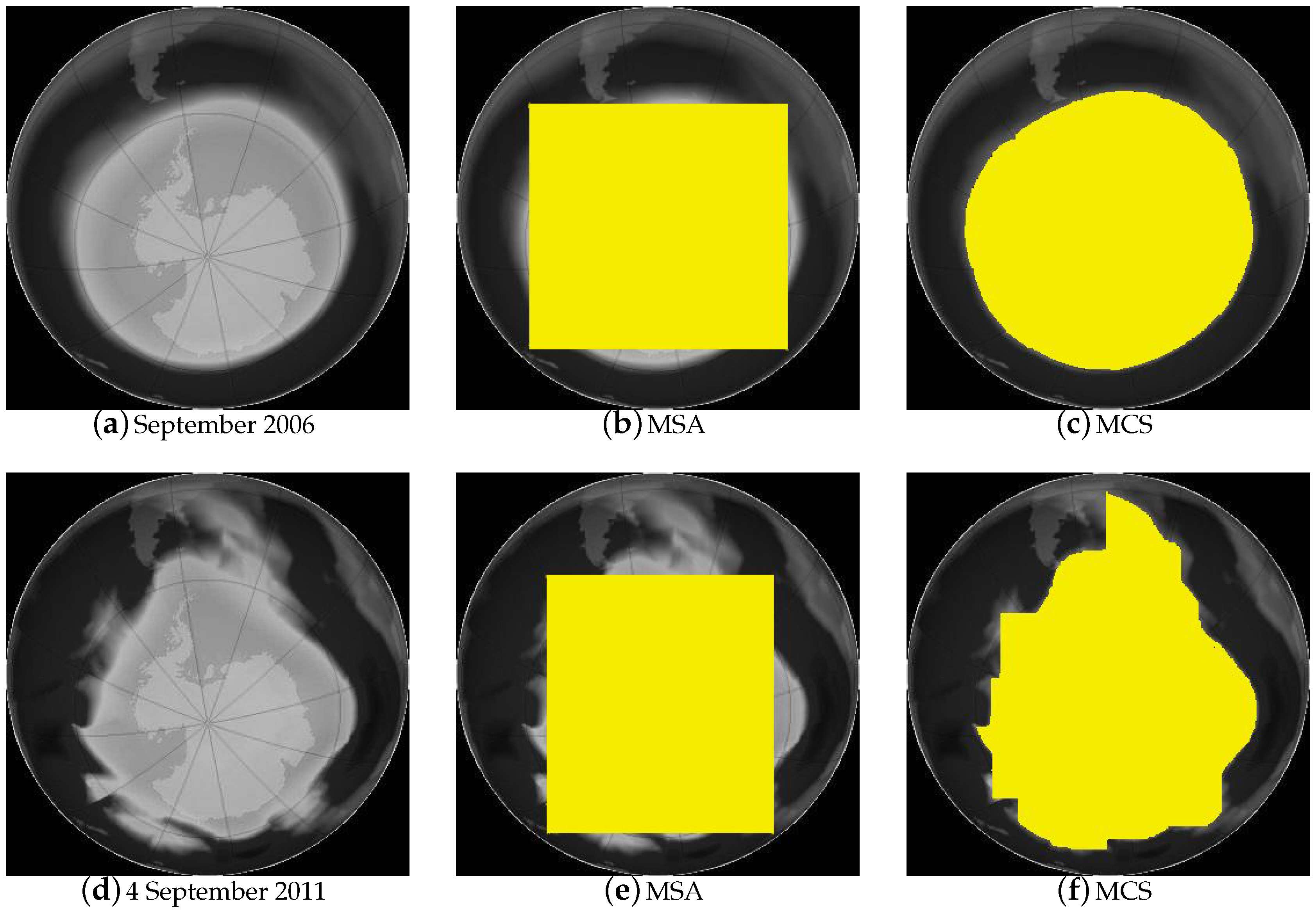
Figure 2.
Two-dimensional architecture.

Figure 3.
Strip-based sequential computation.
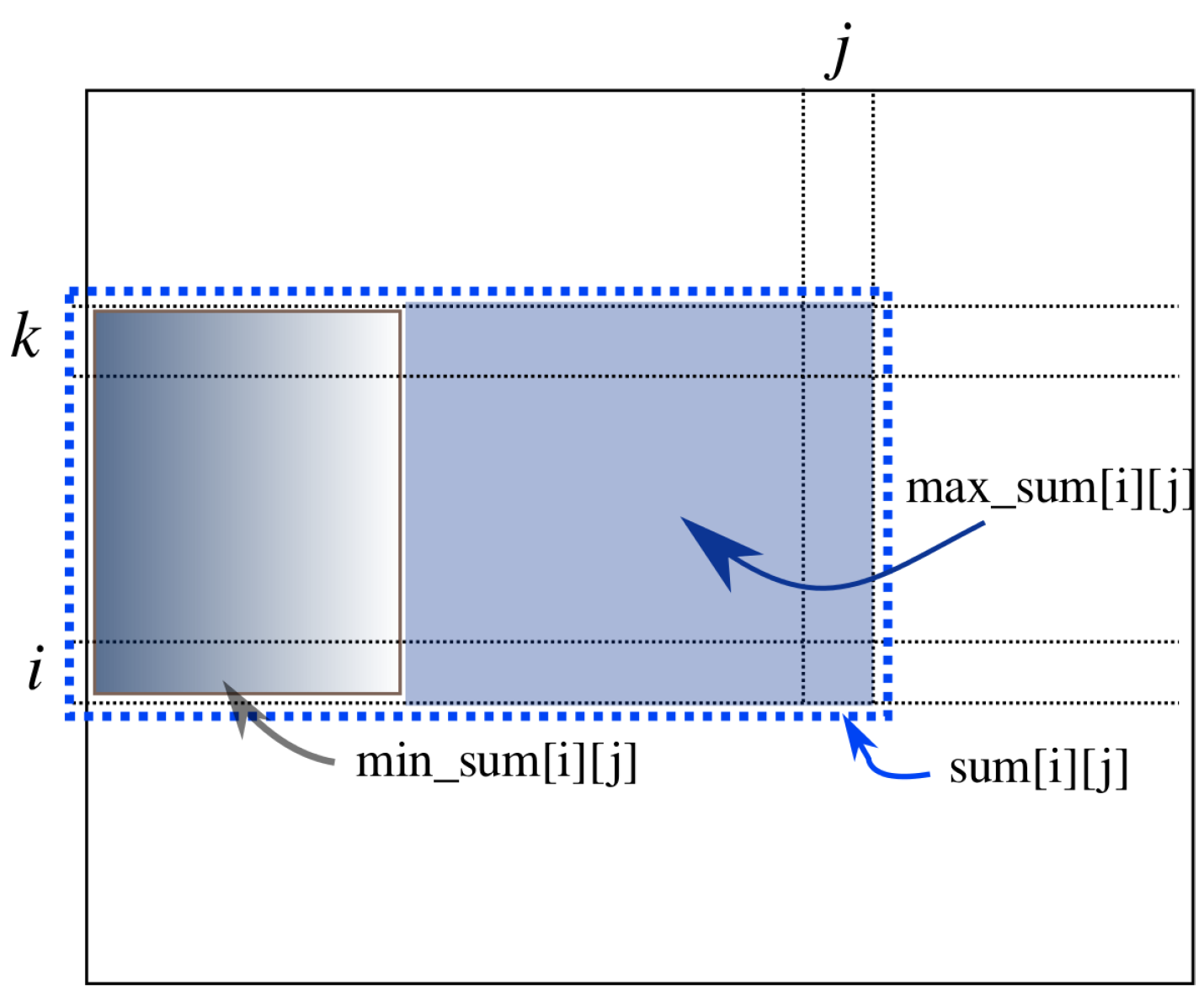
Figure 4.
Illustration for Algorithm 2: The coverage of at step k.
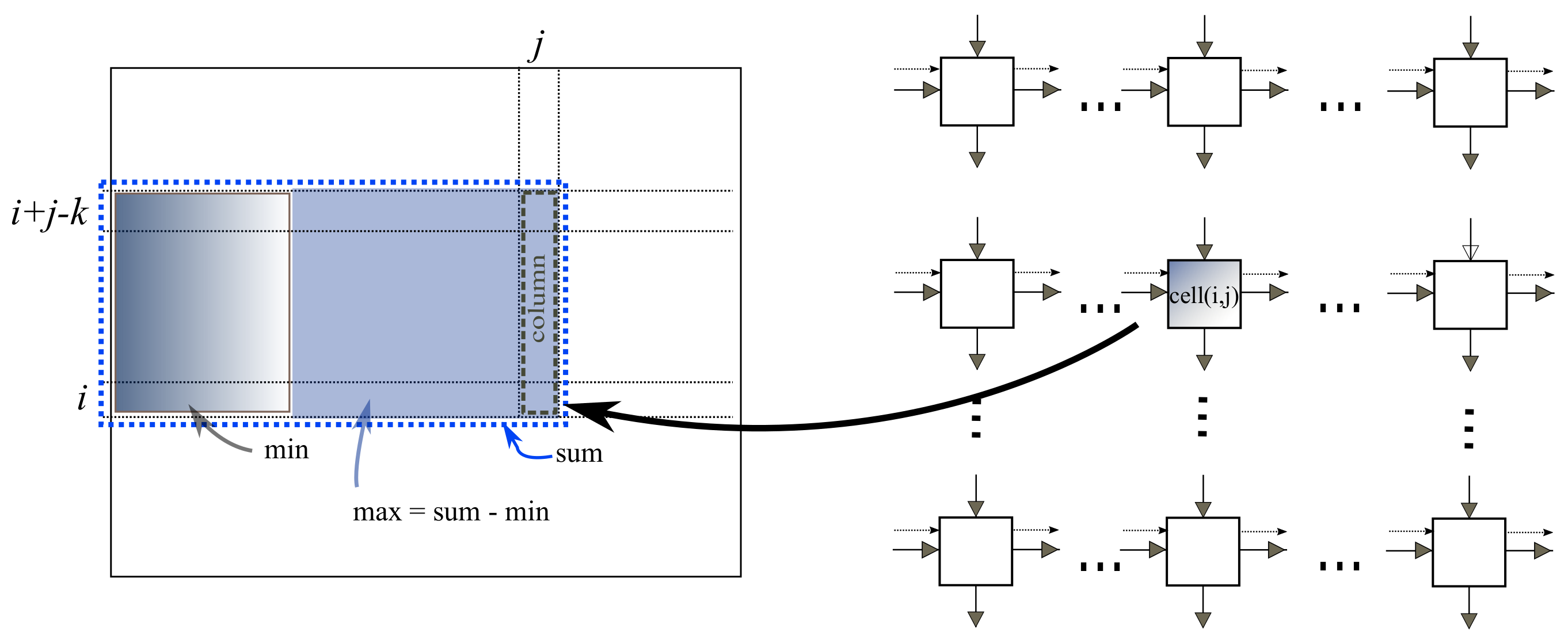
Figure 5.
Illustration for Algorithm 4.
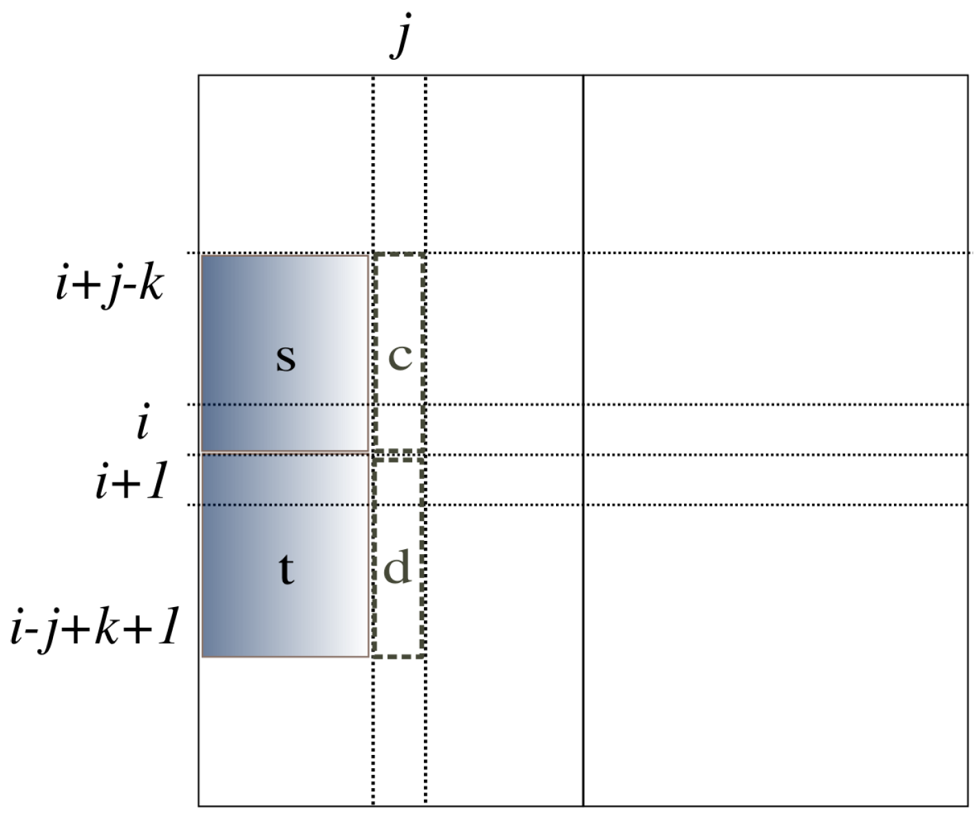
Figure 6.
Sequential computation with position indices i, j, k.

Figure 7.
Three cases for candidates.

Figure 8.
Illustration for Algorithm 8 with position indices and time index k.
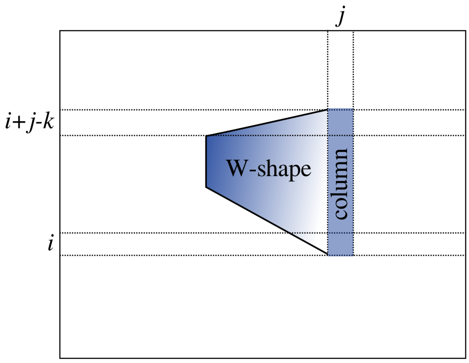
Figure 9.
Maximum finding in 2D mesh.


| = 4 | 16 | 64 | 256 | 1024 | |
|---|---|---|---|---|---|
| n = 64 | 0.1069 | 0.0329 | 0.0258 | 0.0251 | 0.0272 |
| 128 | 0.8435 | 0.2298 | 0.0989 | 0.1253 | 0.1252 |
| 256 | 7.2762 | 1.7506 | 0.4783 | 0.3783 | 0.6088 |
| 512 | 64.5455 | 15.8192 | 3.6038 | 1.3141 | 2.9883 |
| 1024 | 332.8847 | 137.6626 | 33.9193 | 7.7712 | 7.9303 |
| 2048 | x | x | 188.9598 | 87.5153 | 43.5064 |
© 2017 by the authors. Licensee MDPI, Basel, Switzerland. This article is an open access article distributed under the terms and conditions of the Creative Commons Attribution (CC BY) license ( http://creativecommons.org/licenses/by/4.0/).
Share and Cite
MDPI and ACS Style
Bae, S.E.; Shinn, T.-W.; Takaoka, T. Efficient Algorithms for the Maximum Sum Problems. Algorithms 2017, 10, 5. https://doi.org/10.3390/a10010005
AMA Style
Bae SE, Shinn T-W, Takaoka T. Efficient Algorithms for the Maximum Sum Problems. Algorithms. 2017; 10(1):5. https://doi.org/10.3390/a10010005
Chicago/Turabian StyleBae, Sung Eun, Tong-Wook Shinn, and Tadao Takaoka. 2017. "Efficient Algorithms for the Maximum Sum Problems" Algorithms 10, no. 1: 5. https://doi.org/10.3390/a10010005
Note that from the first issue of 2016, this journal uses article numbers instead of page numbers. See further details here.