Multivariate Statistical Process Control Using Enhanced Bottleneck Neural Network


Laboratory of Automatic and Signals-Annaba (LASA), Department of Electronics, Faculty of Engineering, Badji-Mokhtar University, P.O. Box 12, 23000 Annaba, Algeria
*
Author to whom correspondence should be addressed.
Algorithms 2017, 10(2), 49; https://doi.org/10.3390/a10020049
Submission received: 10 March 2017
/
Revised: 24 April 2017
/
Accepted: 24 April 2017
/
Published: 29 April 2017
Abstract
:Monitoring process upsets and malfunctions as early as possible and then finding and removing the factors causing the respective events is of great importance for safe operation and improved productivity. Conventional process monitoring using principal component analysis (PCA) often supposes that process data follow a Gaussian distribution. However, this kind of constraint cannot be satisfied in practice because many industrial processes frequently span multiple operating states. To overcome this difficulty, PCA can be combined with nonparametric control charts for which there is no assumption need on the distribution. However, this approach still uses a constant confidence limit where a relatively high rate of false alarms are generated. Although nonlinear PCA (NLPCA) using autoassociative bottle-neck neural networks plays an important role in the monitoring of industrial processes, it is difficult to design correct monitoring statistics and confidence limits that check new performance. In this work, a new monitoring strategy using an enhanced bottleneck neural network (EBNN) with an adaptive confidence limit for non Gaussian data is proposed. The basic idea behind it is to extract internally homogeneous segments from the historical normal data sets by filling a Gaussian mixture model (GMM). Based on the assumption that process data follow a Gaussian distribution within an operating mode, a local confidence limit can be established. The EBNN is used to reconstruct input data and estimate probabilities of belonging to the various local operating regimes, as modelled by GMM. An abnormal event for an input measurement vector is detected if the squared prediction error (SPE) is too large, or above a certain threshold which is made adaptive. Moreover, the sensor validity index (SVI) is employed successfully to identify the detected faulty variable. The results demonstrate that, compared with NLPCA, the proposed approach can effectively reduce the number of false alarms, and is hence expected to better monitor many practical processes.
1. Introduction
Recently, increasing sensor availability in process monitoring has led to higher demands on the ability to early detect and identify any sensor faults, especially when the monitoring procedure is based on the information obtained from many sensors. Thus, monitoring or control using accurate measurements is very useful to enhance process performance and improve production quality. In the literature, multivariate statistical tools have been widely used to enhance process monitoring [1,2,3,4,5,6,7,8,9,10,11]. Among the popular multivariate statistical process control, the traditional principal component analysis (PCA) and the independent component analysis (ICA) [10,12,13] are the most early and major methods often used in monitoring, which serve as reference of the desired process behaviour and against which new data can be compared (Rosen and Olsson, 2007). However, recent modification of them, such as multiscale PCA, robust NLPCA, kernel PCA, and ICA–PCA combination are used in the literature (Bakshi, 1998, Xiong Li et al., 2007, Zhao and Xu, 2005). Generally, traditional industrial process monitoring relies on the Gaussian assumption of mean and variance which leads to obtaining a confidence limit as constant threshold. However, in practice, the process variables follow approximately mixture Gaussian distributions due to process nonlinearity, which gives a multimodal behaviour; therefore, an adaptive confidence limit (ACL) is expected to improve the process performance. In this context, we propose a robust process monitoring strategy based on Gaussian mixture model (GMM) to extract multiple normal operating modes characterized by m Gaussian components during normal conditions [14,15].
In this work, an enhanced bottleneck neural network (EBNN) is used to estimate the monitored measurements and to classify them according to their probability rates of belonging to various operating modes. Compared to the classical auto-associative neural networks (AANNs) that can be used only for mapping inputs to outputs, the proposed EBNN is not limited to mapping the outputs from input dataset, but also provides a supervised classification of the monitored variables. Then, the kernel density estimation has been adopted to calculate the local confidence limits of the various operating modes, [14,16,17,18].
Subsequently, an ACL is obtained through a weighted sum of the probability rates of each normal mode estimated by the m neurons of the EBNN output layer dedicated to classification and the m Local Confidence Limits of each local .
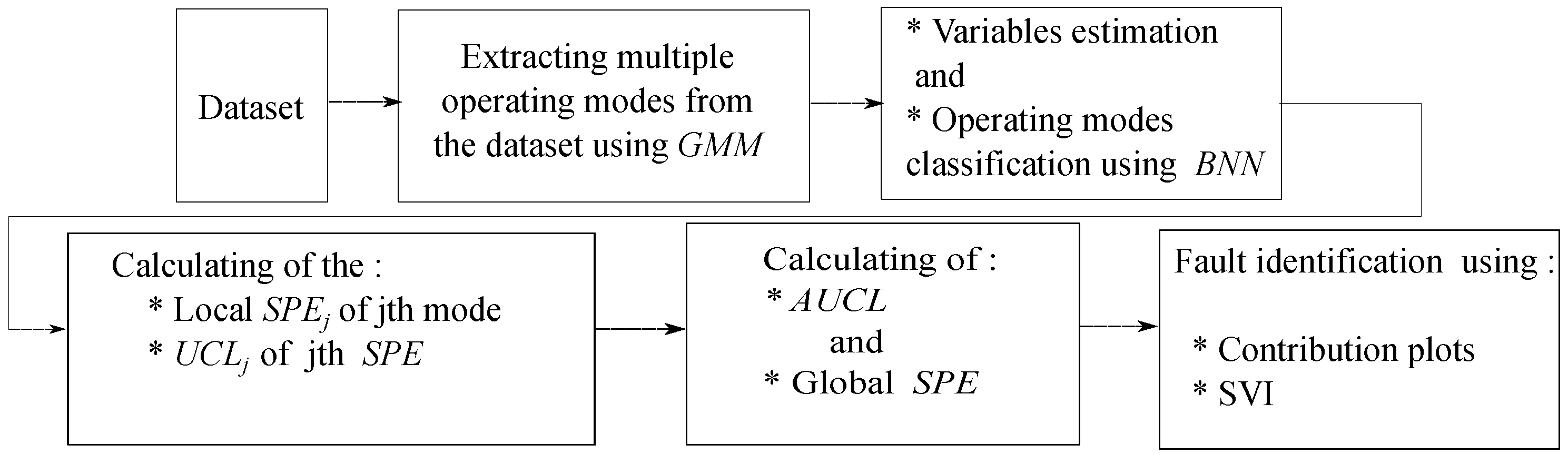
The obtained ACL is associated with the global , which is able to significantly improve the monitoring performance, reduce the false alarms, and detect the onset of process deviations earlier compared to other traditional methods. Traditional contribution plots to the squared prediction error (SPE) are used to isolate the defective sensor. In order to overcome the drawback of the contribution plots, we have successfully proposed a variant of the sensor validity index (SVI) method, which is based on the elimination of the fault on the SPE by reconstructing the faulty variable, the Figure 1 shows a monitoring cycle of the proposed strategy.
The paper is organised as follows: Section 2 introduces the multivariate monitoring tools, including the Gaussian mixture model for calculating the probability rates of normal operating modes, which are used as targets to train the EBNN. Section 3 is dedicated to the case study, in which the effectiveness of the proposed process monitoring strategy is investigated, where we discuss and assess the different results obtained from the used process monitoring tools which are tested on benchmark simulation model no. 1 (BSM1), which is introduced by the working group of the International Water Association (IWA) task group on benchmarking of control strategies for wastewater treatment plants and on actual process. Finally, conclusions are described in Section 4.
2. Materials and Methods
2.1. Multivariate Statistical Process Control
2.1.1. Gaussian Mixture Model
The use of Gaussian mixture models for modelling data distribution is motivated by the interpretation that the Gaussian components represent some general underlying physical phenomena and the capability of Gaussian mixtures to arbitrary shaped densities model densities. This subsection describes the form of the Gaussian mixture model (GMM) and motivates its use as a representation of historical data for advanced statistical process monitoring (SPM). The use of Gaussian mixture density for process monitoring is motivated by two interpretations. First, the individual component Gaussians are interpreted to represent some operating modes or classes. These classes reflect some underlying phenomena having generated data; for example, hydrological or biological in water treatment plants. Second, a Gaussian mixture density is shown to provide a smooth approximation of the underlying long-term sample distribution of observations collected from industrial plants. The GMM parametrization and the maximum-likelihood parameter estimation are described. Multiple operating modes in normal process conditions can be characterized by different Gaussian components in GMM, and the prior probability of each Gaussian component represents the percentage of total operation when the process runs at the particular mode [19,20]. The probability density function of Gaussian mixture model is equivalent to the weighted sum of the density functions of all Gaussian components as given below:
where , denotes the prior probability of the Gaussian component and is the multivariate Gaussian density function of the component. For each component, the model parameters to be estimated are and , the latter of which include the mean vector and the covariance matrix (Duda et al., 2001). During the model learning, the following log-likelihood function is used as objective function to estimate the parameter values
where is the training sample among the total N measurements.
The Gaussian mixture model can be estimated by Expectation-Maximization algorithm through the following iterative procedure:
- E-Step: compute the posterior probability of the training sample at the iterationwhere denotes the Gaussian component.
- M-Step: update the model parameters at the iteration
It should be noted that the number of Gaussian components corresponds to the number of operating modes in normal conditions [21]. The next phase after extracting the mixture operating modes consists to design the EBNN model.
2.1.2. Enhanced Bottleneck Neural Network
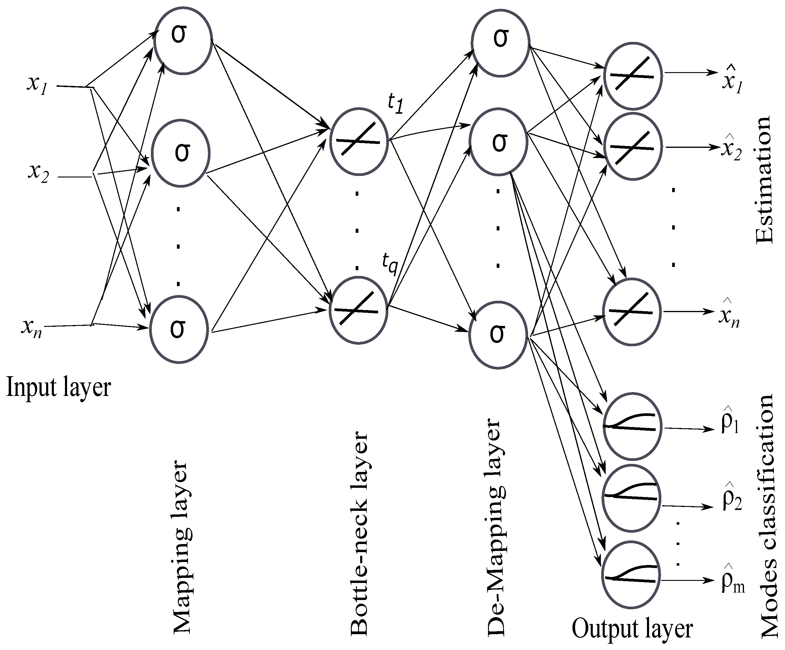
Auto-associative neural networks are powerful tools for mapping inputs to outputs, especially when this mapping is nonlinear. In this work, an enhanced bottleneck neural network (EBNN) topology is used that includes five layers with three hidden layers: mapping layer, bottleneck layer, and de-mapping layer, the input and output variables [13,22,23]. Once the general structure is defined, it remains to determine the necessary number of neurons in each hidden layer. This number is generally determined by cross-validation. In addition, the classification using feedforward artificial neural networks is an effective tool to produce a specific output pattern for a specific input pattern. For this purpose, a small artificial neural network classifier (ANNC) is included in the output layer of EBNN (part dedicated to estimating the probability rates of normal operating modes) as shown in Figure 2. ANNC is used because of its ability to estimate the probability rates of the monitored variables, leading to their classification according to their operating modes. In the training phase, the number of normal operating modes to be extracted is assumed to be known.
The training of the whole network includes two steps:
- Encoding process (compression): For an input vector , the encoding process (compress inputs) can be described as:When the bottleneck layer forces the EBNN to compress the inputs (variables to be monitored).
- Decoding process (decompression): The bottleneck layer produces the network outputs (estimation and classification) by decompression, which is given as:with
- -
- n is the number of neurons in the input layer.
- -
- h is the number of neurons in the mapping layer.
- -
- q is the number of neurons in the bottleneck layer.
- -
- w is the weight values of the network.
- -
- is the threshold value for the node of the mapping layer.
- -
- m is the number of neurons in the output layer of the operating modes classification part.
- -
- is the sigmoid transfer function,
where the transfer function in the mapping and de-mapping layers is sigmoid, and in bottleneck and output layers is linear. Exceptionally, in the output classification part is log-sigmoid in order to generate a posterior probability rates vary between 0 and 1.
The gradient descent algorithm is adopted to train the BNN and to find the optimal values [24,25]. This is done iteratively by changing the weights w and threshold (randomly initialized before the training) according to the gradient descent so that the difference between the ideal output and the real output is the smallest. The training process is finished when the cost function E for all samples is minimized, which is calculated as:
where
- -
- N is the number of training samples.
- -
- n is the number of neurons in the output layer of the estimation part.
- -
- m is the number of neurons in the output layer of the modes classification part.
the variables estimation part:
- -
- is the n desired values of the output neuron.
- -
- is the n actual outputs of that neuron.
the modes classification part:
- -
- is the probability rate already obtained with GMM of the mode.
- -
- is the actual output of neuron which corresponds to jth mode.
It should be noted that the number of neurons in the output layer of the modes classification part corresponds to the extracted normal operating modes.
2.2. Process Monitoring and Diagnosis
2.2.1. Squared Prediction Error
The difference between the enhanced BNN inputs and their estimated values can be used as an indicator to judge the occurrence of the abnormal events and their severity. Several multivariate extensions of fault detection approaches have been proposed in literature; the univariate statistic SPE, which is established using the error that follows a central Chi-squared distribution [9,26] has a fundamental importance for process monitoring because it indicates the changes in the correlation structure of the measured variables. Its expression at the instant k is given by:
where;
In offline stage, once the EBNN model is designed, it should be noted that m local and must be calculated in residual subspace for the various operating modes.
In online phase, the global (which is multimodal) provides fault detection in residual space. The process is considered in abnormal operating state at the observation if the global :
with is the adaptive upper control limit of the global .
2.2.2. Adaptive Upper Control Limits
Once the constants of each and the probability rates of each operating mode are calculated, an adaptive upper control limit can be obtained according to the following formula:
where
- -
- m is number of Gaussian components corresponding to the normal operating modes.
- -
- is the probability rate of mode during the normal operating regime.
- -
- is the upper control limit using the kernel density estimation (KDE) of each mode during the normal operating regime.
- -
- n is the number of samples.
2.2.3. Upper Control Limit by KDE
is a powerful data-driven technique for the nonparametric estimation of density functions [27,28,29]. Given a sample matrix with n variables and l samples , a general estimator of the density function can be defined as:
where is the bandwidth matrix, indicates the determinant of H, and is the kernel function, where the kernel estimator is the sum of the bumps placed at the sample points. The defines the shape of the bumps, while the bandwidth defines the width. A popular choice for is the Gaussian kernel function:
The critical issue for determining is the selection of bandwidth matrix H. In order to determine H, we must first determine its matrix structure. Generally, there are three possible matrix structure cases:
- (1)
- a full symmetrical positive definite matrix with parameters —for example, in which = ;
- (2)
- a diagonal matrix with only l parameters, ;
- (3)
- a diagonal matrix with one parameter, , where, I is unit matrix.
According to [30], the first case is the most accurate, but is unrealistic in terms of computational load and time, while the third case is the simplest but can cause problems in certain situations due to the loss of accuracy by forcing the bandwidths in all dimensions to be the same. In this study, the second matrix structure bandwidth will be studied as a compromise of the first case and the third case, and an optimal selection of bandwidth matrix algorithm will be used [31].
The above approach is able to estimate the underlying probability density function (PDF) of the matrix. Thus, the corresponding upper control limit can be obtained from the of the matrix with a given confidence bound by solving the following equation:
where is the probability density function of for normal operating data, is the confidence level, and are the local .
Therefore, the KDE is a well-established approach to estimating the PDF, particularly for random variables like which are univariate although the underlying processes are multivariate.
2.3. Fault Isolation
After detecting a fault, it is necessary to identify which sensor becomes faulty. In this section, we re-examine the concept of contribution plots and SVI based on nonlinear reconstruction.
2.3.1. Isolation by Contribution Plots
The contribution plot is the most conventional method that has been widely used in fault isolation approaches. This method is generally based on the contribution rate of each variable to indicate which variable has an extreme contribution to the . These contributions can be calculated as:
2.3.2. Sensor Validity Index
This approach is applied when a fault sensor is detected. Thus, it consists of reconstructing its measurement using the EBNN model which was already trained in normal operating conditions. Therefore the isolation is performed by calculating the indicators of each measurement ( is the number of sensors) after the reconstruction of all sensors. It is noted that the reconstruction of the faulty sensors eliminates the abnormal condition; we must also remember that the indicator of the faulty sensor calculated after reconstruction is below its adaptive upper control limit compared to the of other variables, which are all above their respective [32].
The reconstructed measurement can be obtained iteratively, estimated, and re-estimated (re-injected) by EBNN model until convergence as indicated in Figure 3.
The SVI is based on the reconstruction principle, which consists to suspect a faulty sensor and reconstruct (or correct) the value of the faulty sensor based on the EBNN model already performed and the other measurements of all sensors; the procedure is repeated for each sensor. The identification is performed by comparing the SVIs before and after reconstruction. The sensor validity index is a measure of sensor performance; it should have a standardized range regardless of the number of principal components in the bottleneck layer, noise, measurement variances, or fault type. The ratio of and the global SPE can provide these desired properties for the identification of a sensor fault [4]). The SVI can be calculated as:
where the SPE is the global squared prediction error calculated before reconstruction and SPE is the sensor calculated after reconstruction, [33,34,35].
3. Case Study : Wastewater Treatment Plant (WWTP) Monitoring
The main purpose in biological wastewater treatment is to transform nitrogen compounds in order to remove them from wastewater, where admissible concentrations of these harmful pollutants are defined by European standards. In order to generate a limit for the toxic organic chemicals which have recently caused a lot of harm both to human beings and the environment, stringent laws have been increasingly imposed on the quality of wastewater discharged in industrial and municipal effluent. This rising concern about the environmental protection leads the wastewater treatment plants (WWTPs) to the necessity of running under normal operating conditions. To improve the operating performance of wastewater treatment plants like all industrial processes, an on-line monitoring system equipped with electronic sensors is necessary for early detection and identification of any abnormal event affecting the process [36,37]. The proposed strategy is applied to the simulated wastewater treatment process BSM1 and to the real-process, where many sensor are prone to malfunctions [38,39,40].
3.1. Simulated Process Case
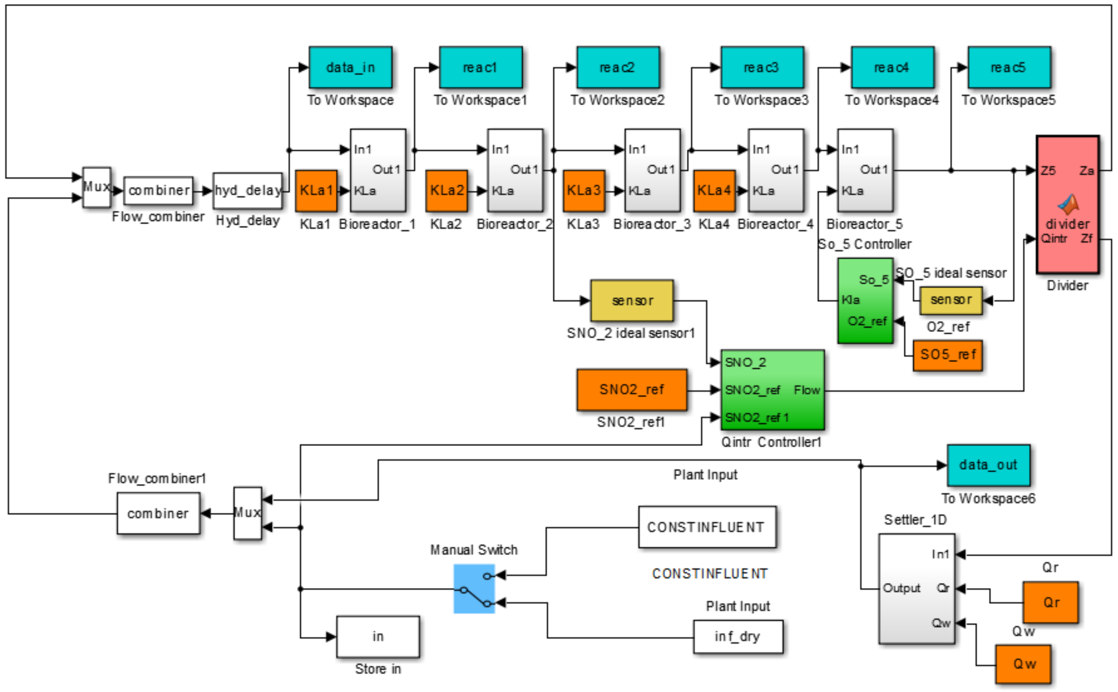
This benchmark plant is composed of a five compartment activated sludge reactor consisting of two anoxic tanks followed by three aerobic tanks (see Figure 4). The plant thus combines nitrification with pre-denitrification in a configuration that is commonly used for achieving biological nitrogen removal in full-scale plants. The activated sludge reactor is followed by a secondary settler. The simulated wastewater treatment process BSM1 (Figure 5) is used under dry weather during 7 days under normal operating conditions. The sampling period is 15 min, where the training dataset is composed of 673 observations and 672 observations are used for the test phase. The plant is designed for an average influent dry-weather flow rate of 18,446 md and an average biodegradable chemical oxygen demand (COD) in the influent of 300 g·m. For more details, the simulated wastewater treatment process BSM1 is available on [41].
The monitored sensors of the BSM1 used in this work are given in Table 1.
3.2. Real Process Case
In order to illustrate the effectiveness of the proposed strategy, the monitoring approaches have been tested on real data collected from an actual wastewater treatment process of Annaba, situated in the North-East Algeria (450 km of Algiers and 8 km east of Annaba city), where the real data contains 1300 observations of some sensors (see Table 2) in normal operating conditions, with a medium flow of 83,620 m/day and peak flow during dry weather 5923 m/h.
The purification process used is activated sludge, and has two principal treatment sectors; the primary includes bar racks, grit chamber, de-oiling, and sand filters, whose objective is the removal of solids. The secondary sector is made for removing the organic matter present in the influent wastewater, where the organic matter pollutants serve as food for microorganisms. This is done by using either aerobic or anaerobic treatment processes. The schematic of the used actual plant is shown in Figure 6. The monitored sensors in this work are given in Table 2.
3.3. Results and Discussion
This section presents a simulation study with some comments about the obtained results to examine the effectiveness of the proposed strategy for on-line process monitoring applied to simulated wastewater treatment process BSM1 and to real data.
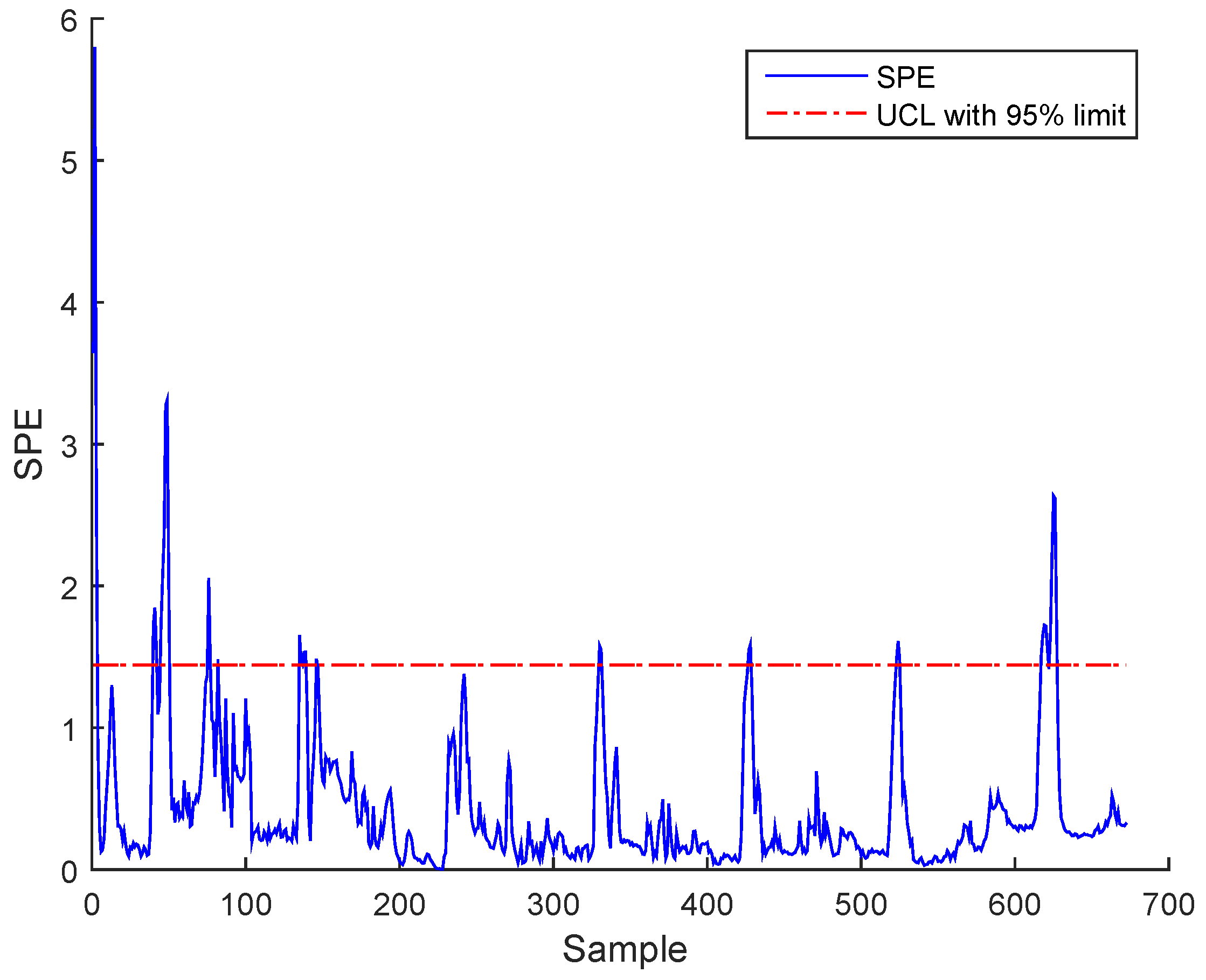
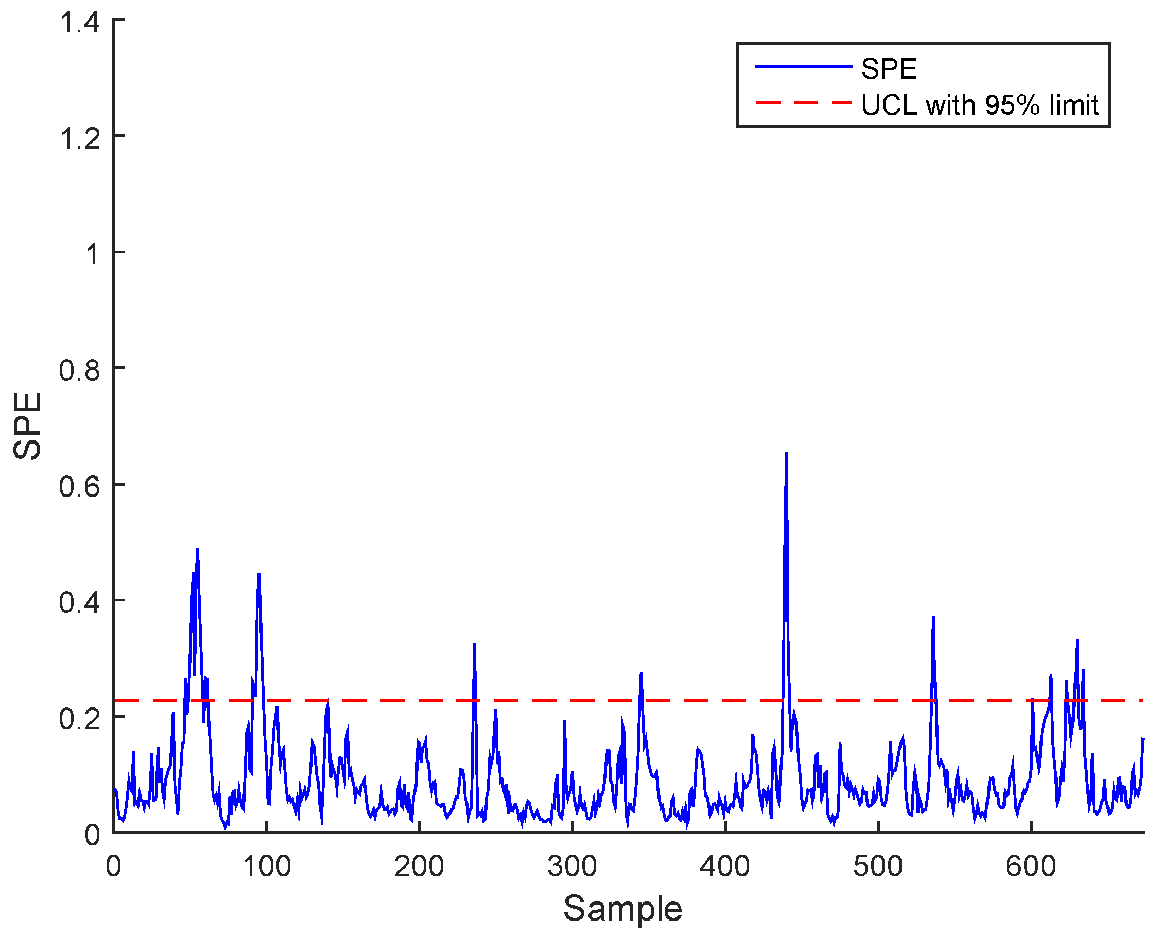
In order to illustrate the advantages of the AUCL based on EBNN compared to two base-line multivariate statistical monitoring methods (namely the nonlinear PCA (NLPCA) and ICA), simulation tests were carried out on BSM1 and on actual data. Figure 7 and Figure 8 show the SPE during normal conditions using ICA of BSM1 data and real data, respectively. The upper control limit (UCL) was made constant.
Figure 9 and Figure 10 present the SPE using the traditional NLPCA based on AANN with a constant UCL of the BSM1 data and real data, respectively. The high number of false alarms can be seen. In the following part of this section, the results of the proposed method using UACL based on EBNN show the effectiveness in overcoming this drawback.
Before the construction of EBNN, a normalization of the monitored variables is necessary. Each variable of the training and testing data matrices are centred and scaled by subtracting and dividing, respectively, the mean/standard-deviation from/by each column to render the results independent of the used units.
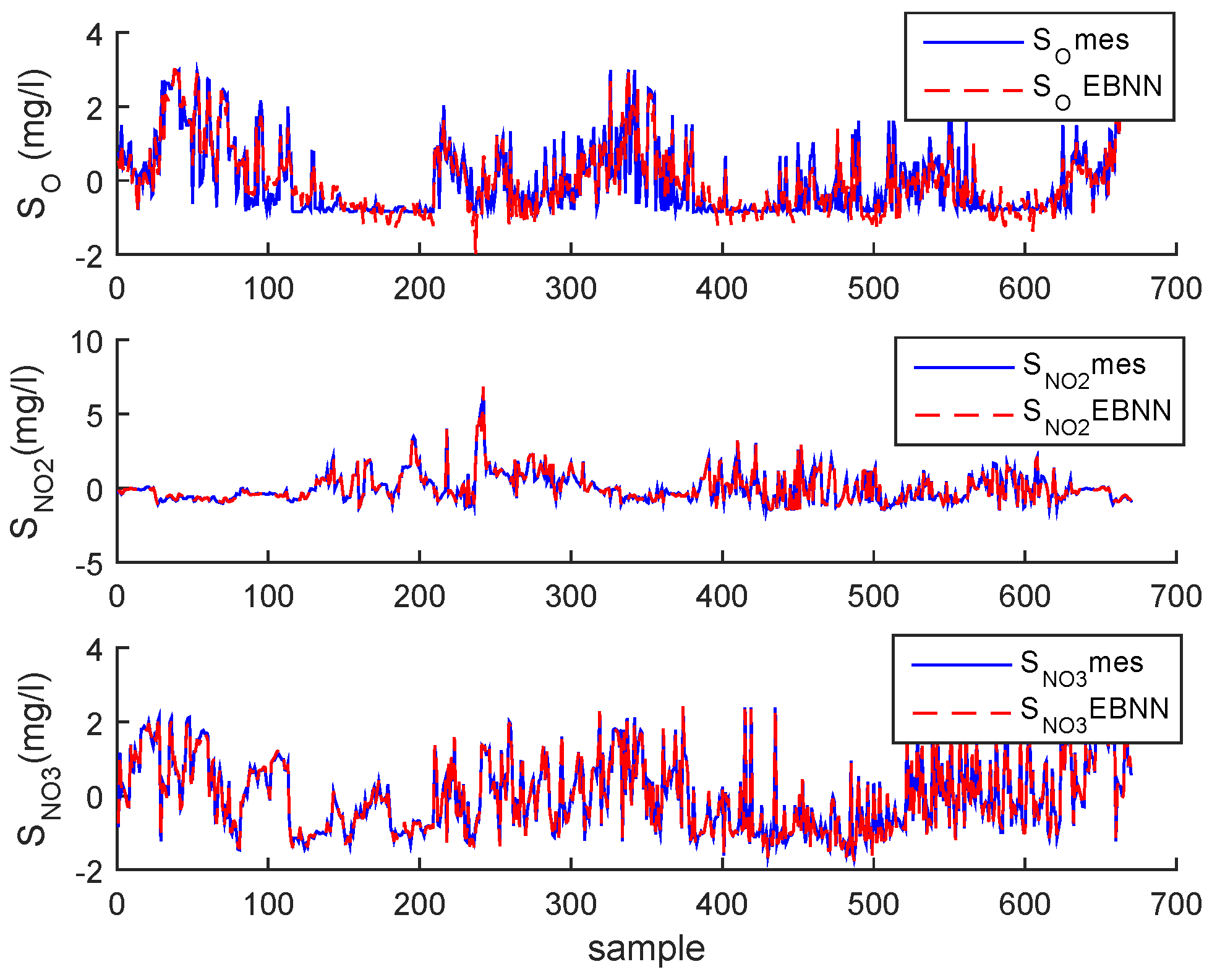
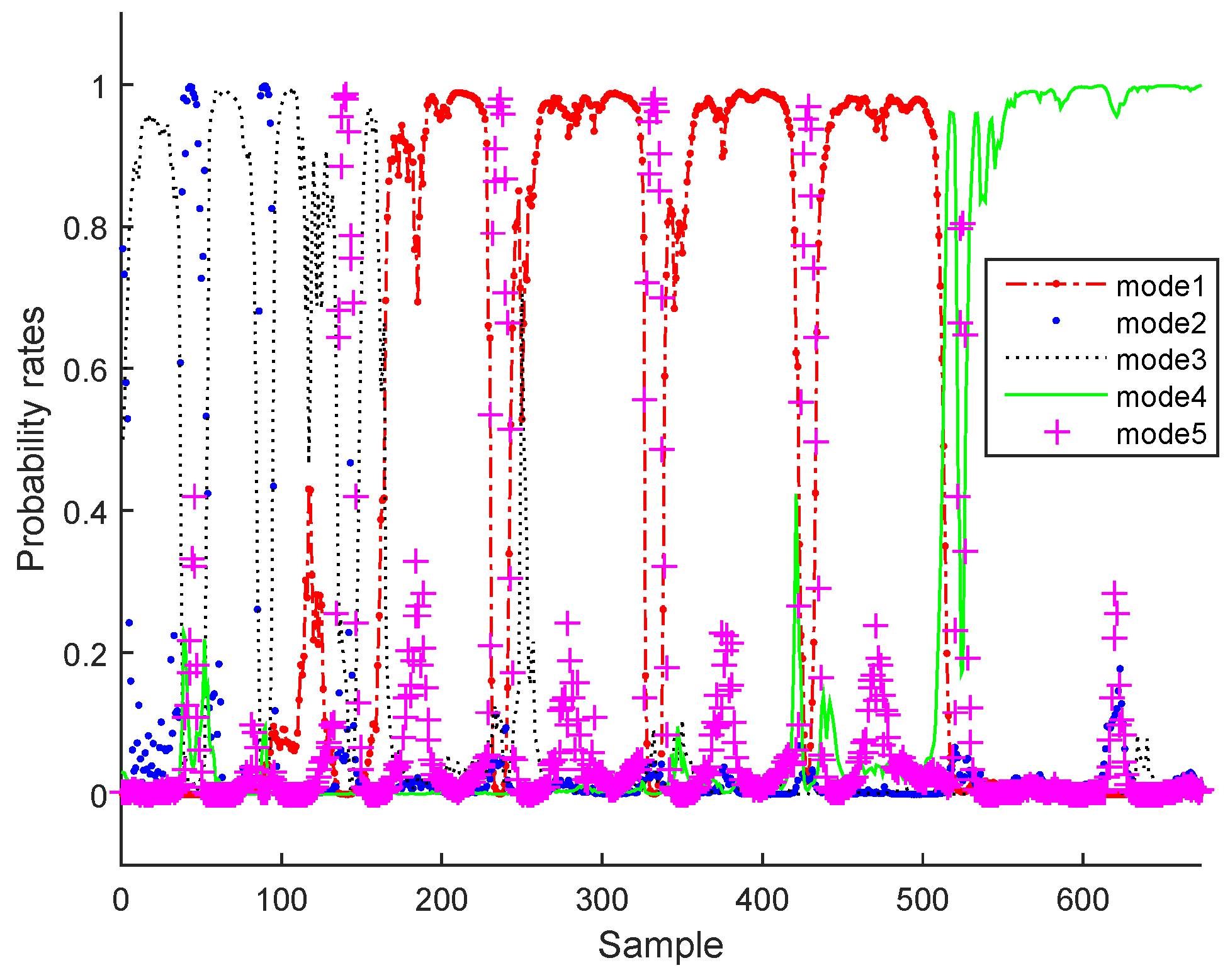
In the testing phase under normal operating conditions, as illustrative examples, three of the estimated variables and the output classified modes (for q = 5 the number of components in bottleneck layer and m = 5 the number of normal operating modes) are plotted in Figure 11 and Figure 12 for the BSM1 case and Figure 13 and Figure 14 for real data, respectively.
It can be clearly seen that the monitored variables have been reconstructed and the probability rates are successfully estimated.
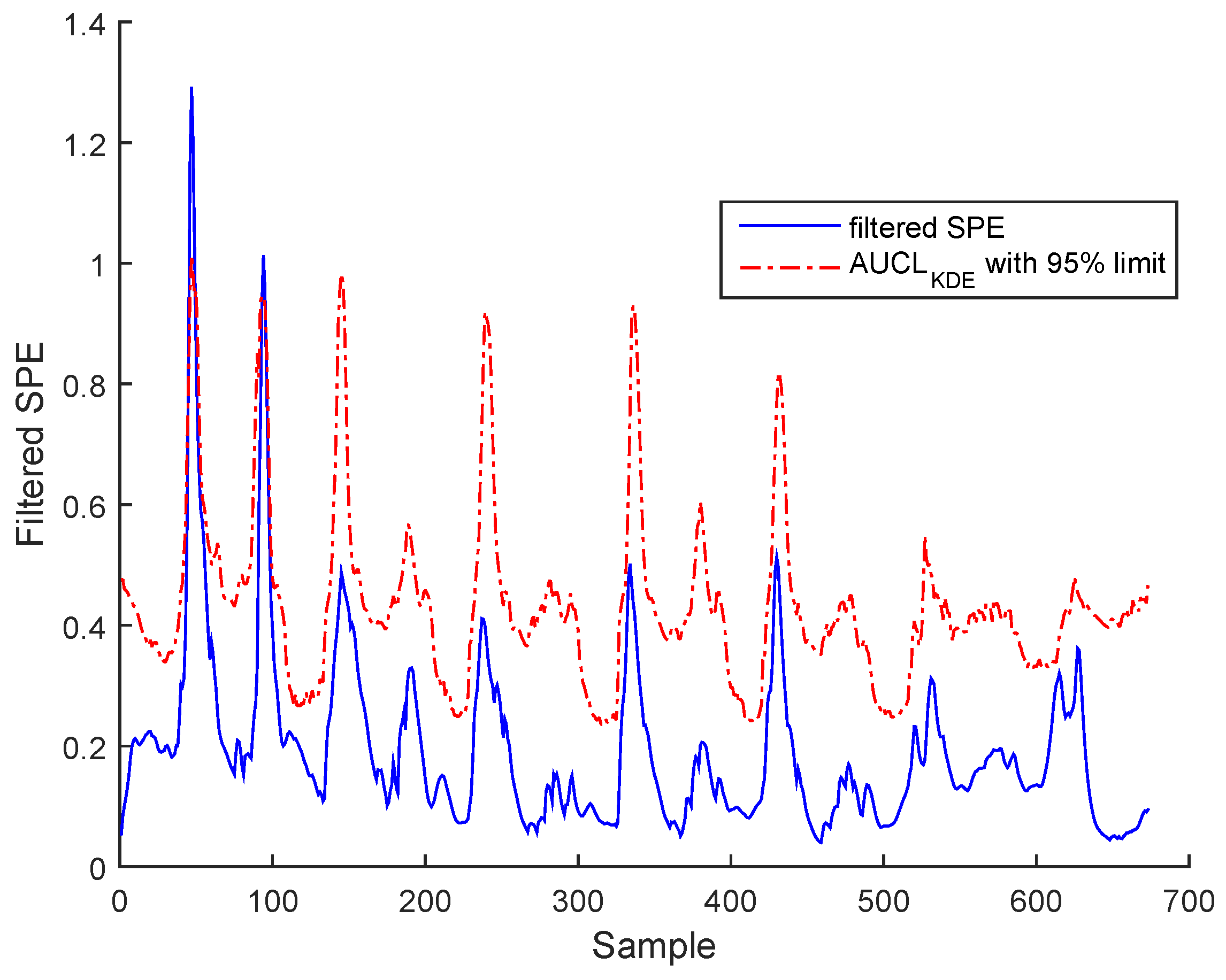
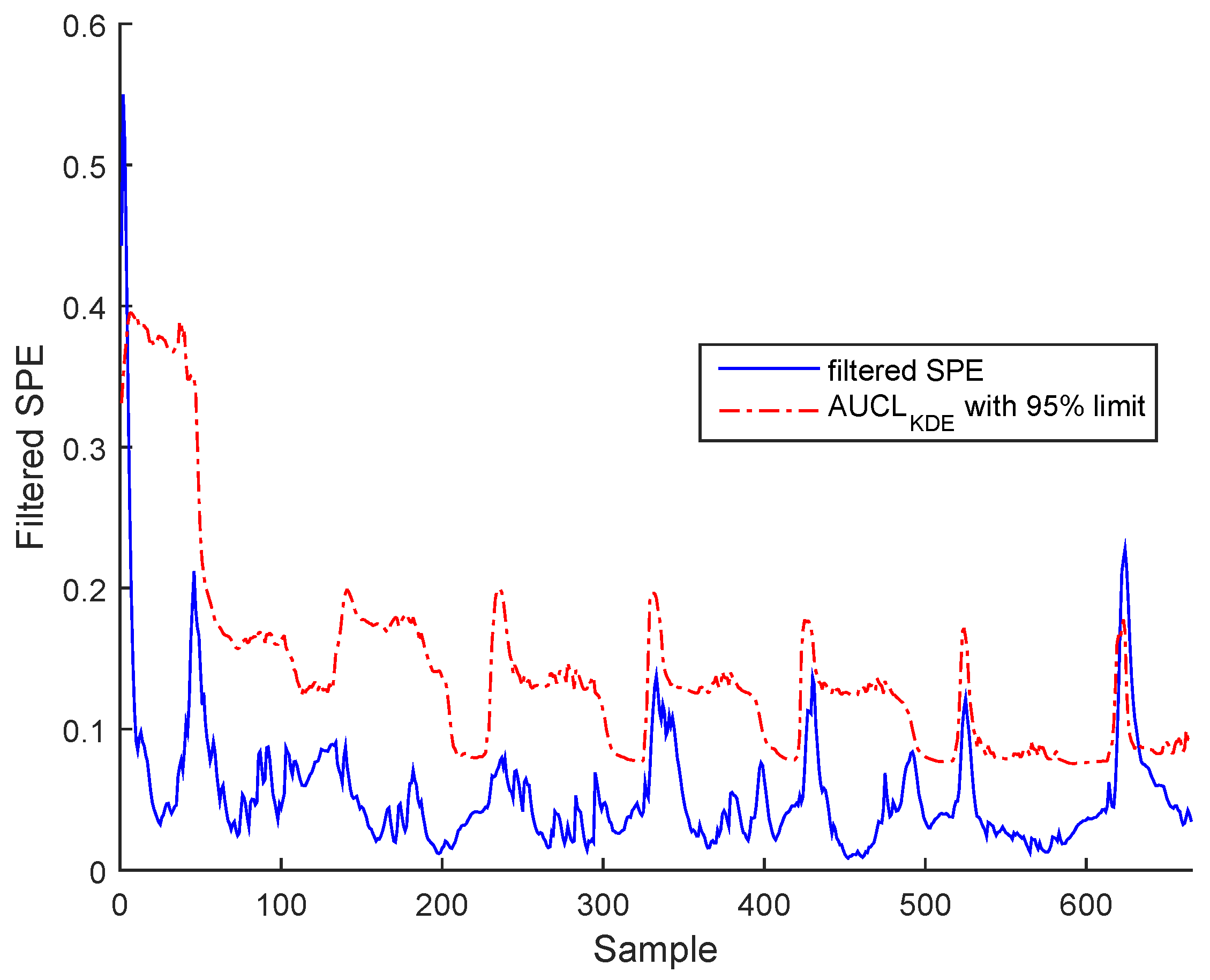
Figure 15 for BSM1 data and Figure 16 for real data represent the evolutions of the filtered SPE for BSM1 and real data, respectively, with an AUCL using KDE at a confidence level of under normal operating conditions. To reduce the false alarms, an exponentially weighted moving average (EWMA) is used to filter the effect of outliers and noise, as shown in figures of the filtered SPE.
The formulation of the process monitoring strategy of this work focuses on the problem of faulty sensors precisely in WWTP, which may exhibit partial failures such as precision degradation due to significant noise, bias, or drift due to sludge clogging [42,43], which can be defined below:
- a- Precision degradation: The precision degradation model is defined as a Gaussian random process with zero mean and unknown covariance matrix.
- b- Bias: The bias error evolution can be characterized by positive or negative value.
- c- Drift: This error follows an increasing deviation, such as polynomial change.
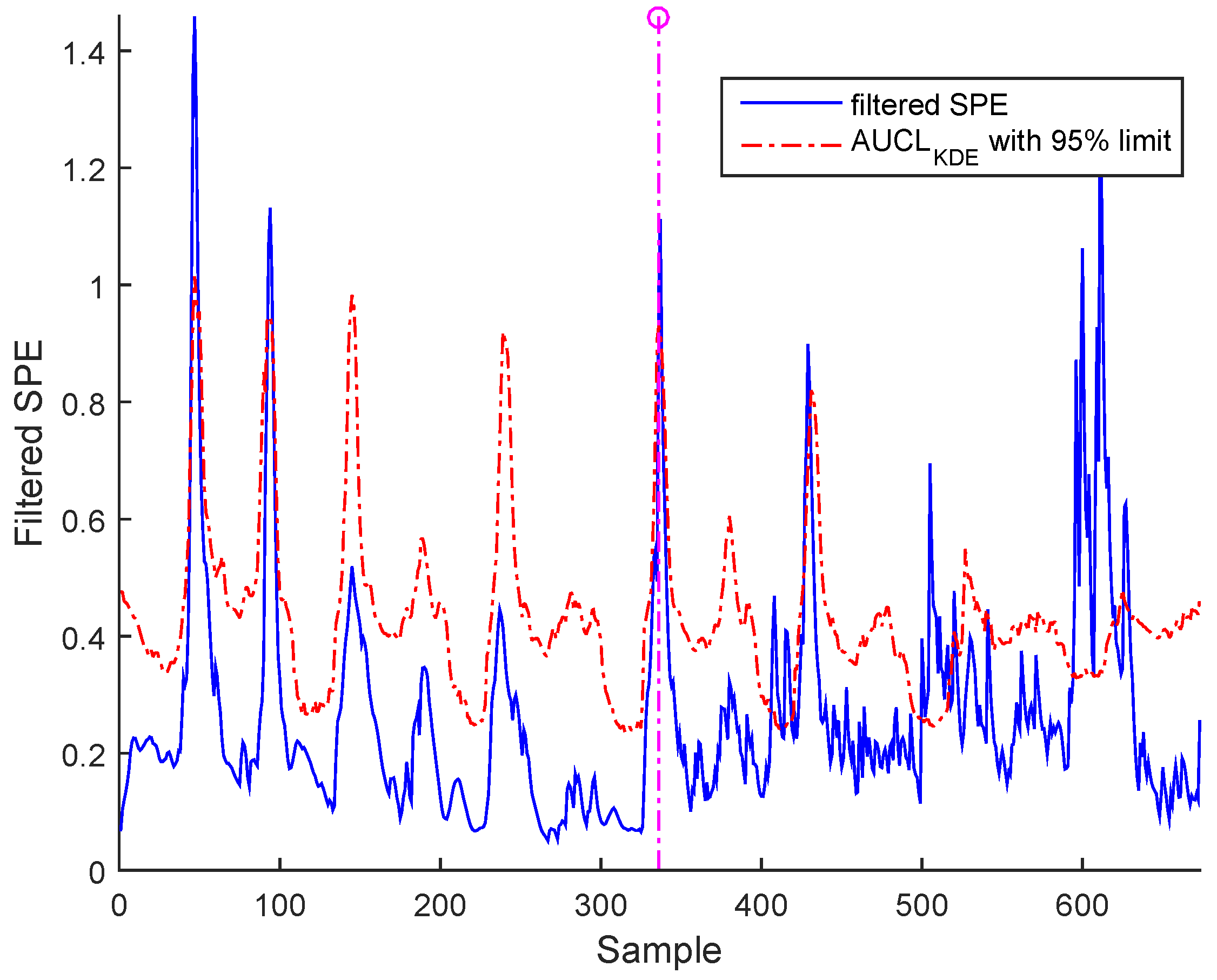
Figure 17 and Figure 18 show the results from a precision degradation fault tested on both cases of data, where the filtered SPE moves up and down many times above its AUCL.
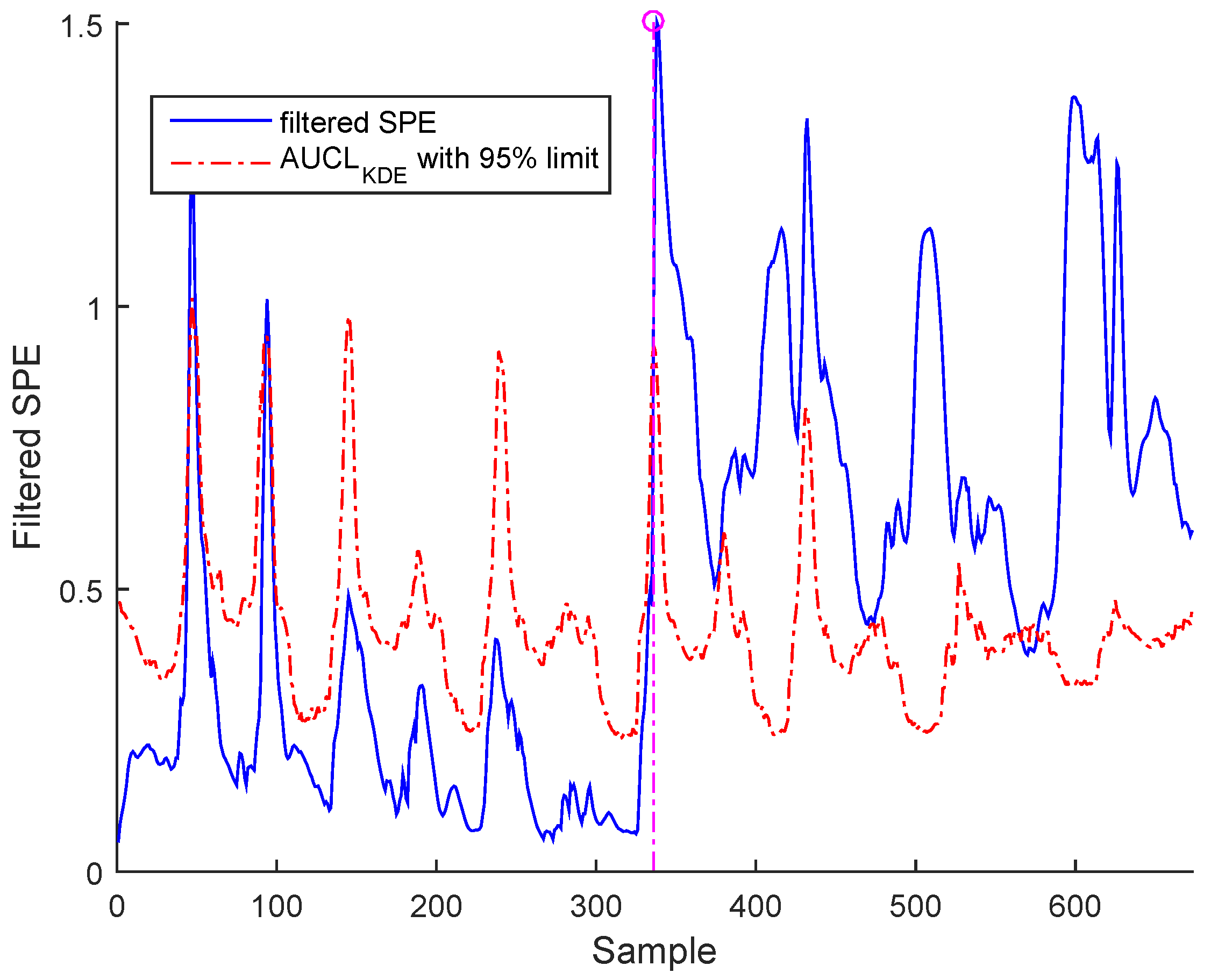
Bias fault can be detected by filtered SPE, as shown in Figure 19 for BSM1 data and Figure 20 for real data.
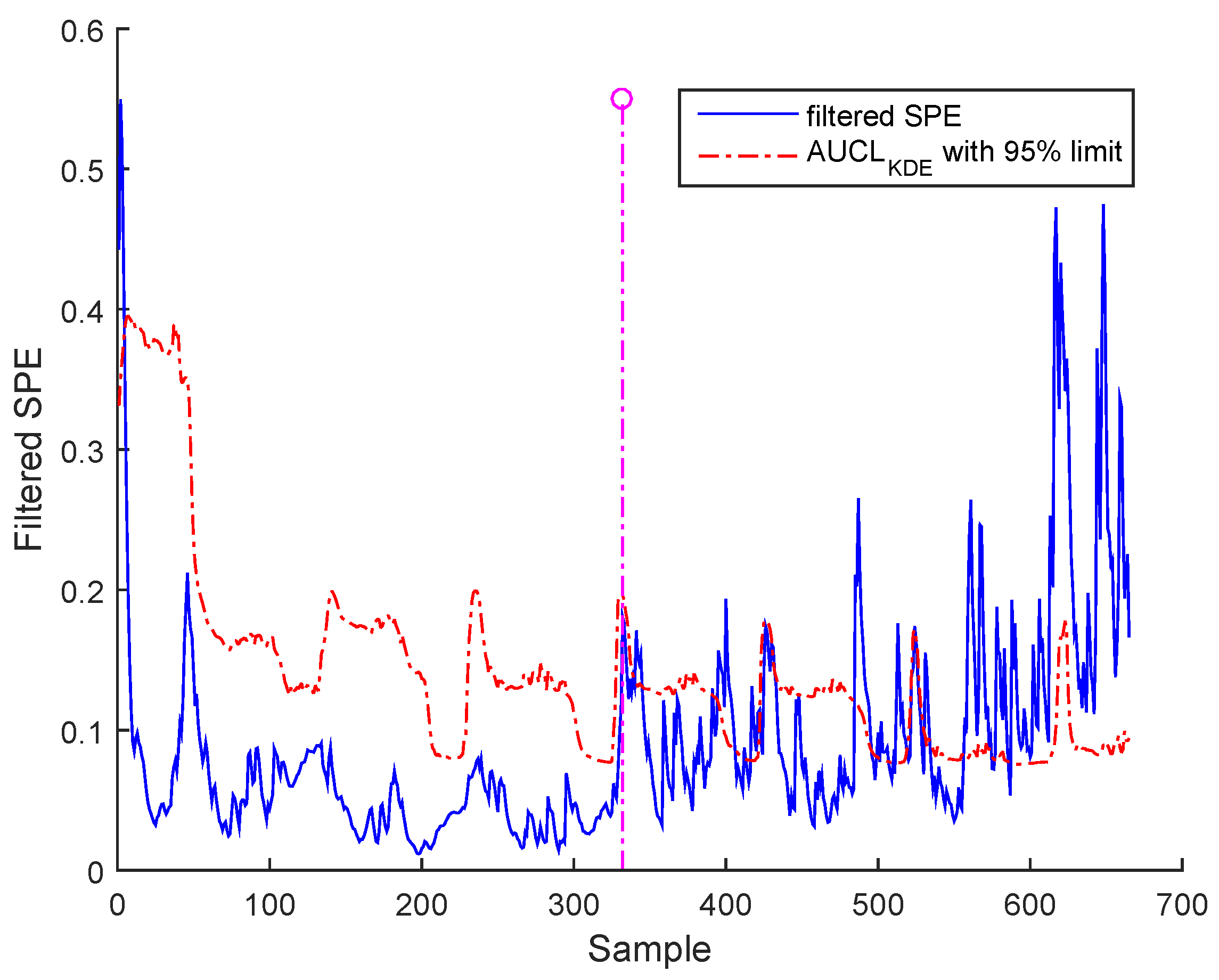
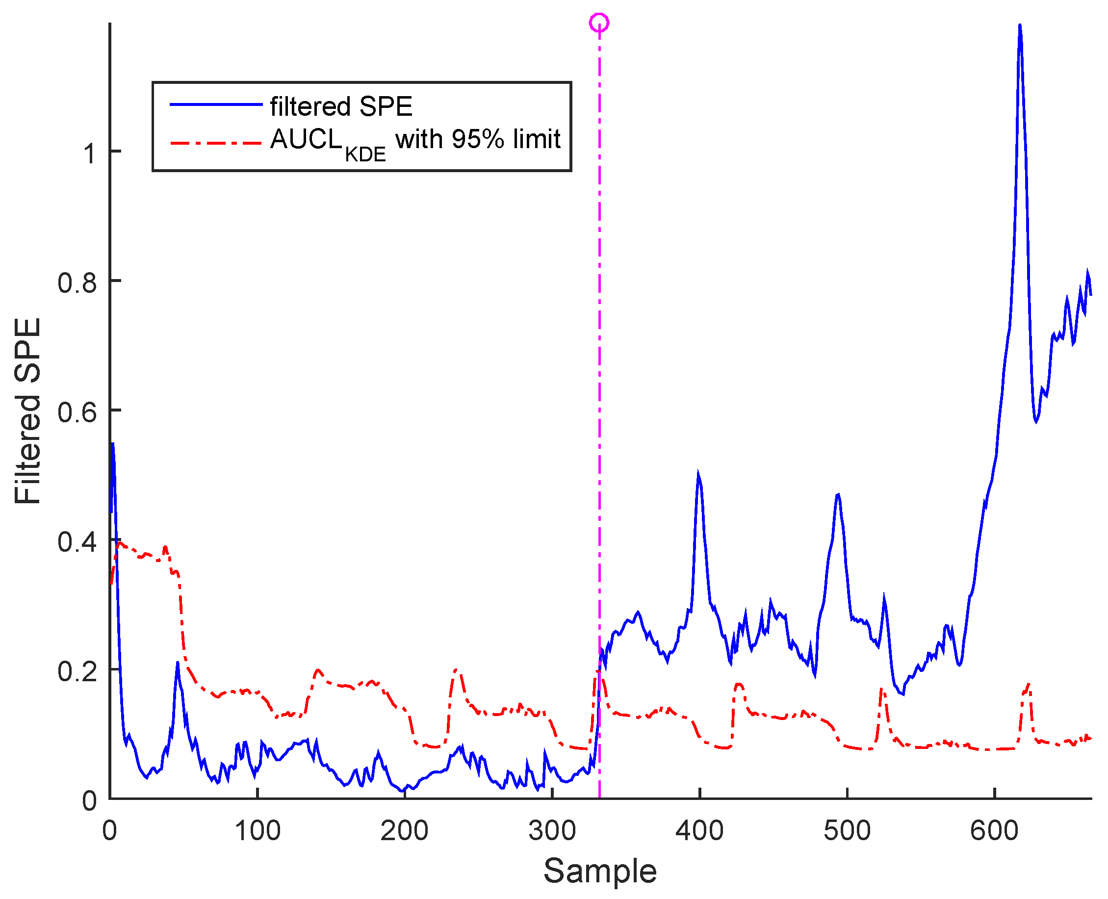
The last simulation test concerns the drift fault, which can also be detected by filtered SPE, as indicated in Figure 21 and Figure 22 for BSM1 data and real data, respectively.
It is worth noting that the selected abnormal events correspond, respectively, to precision degradation, bias, and drift malfunctions related to the sensors of dissolved oxygen, nitrate, and nitrite nitrogen, which are the most important sensors in WWTP. However, represents a high correlation with the other variables. It can be seen that the SPE indicator exceeds its adaptive upper control limit in the case of bias and drift faults; however, in the precision degradation case, it can be seen that this malfunction type is translated by discontinuous alarms despite the use of AUCL. It is clear that the different faults are detected at various samples according to the type of fault, as indicated in Table 3. The results show the proposed robust monitoring performance in the presence of faults and produces few alarms. For identification, we cannot observe anything in the previous figures.
Sensor Fault Identification and Reconstruction
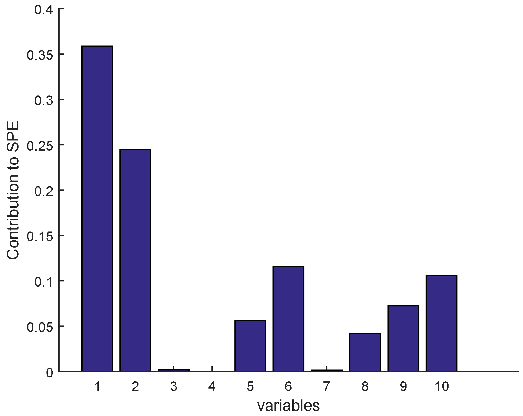
Once a fault is detected, it is necessary to identify the faulty sensor according to the contribution plots approach, as given in Figure 23 and Figure 24 for BSM1 data and real data, respectively (drift fault case), where in the detection moment the sensor having the largest contribution to the SPE is the faulty sensor. To overcome the drawbacks of the traditional contribution plots, identification via reconstruction is proposed, as illustrated in the figures below.
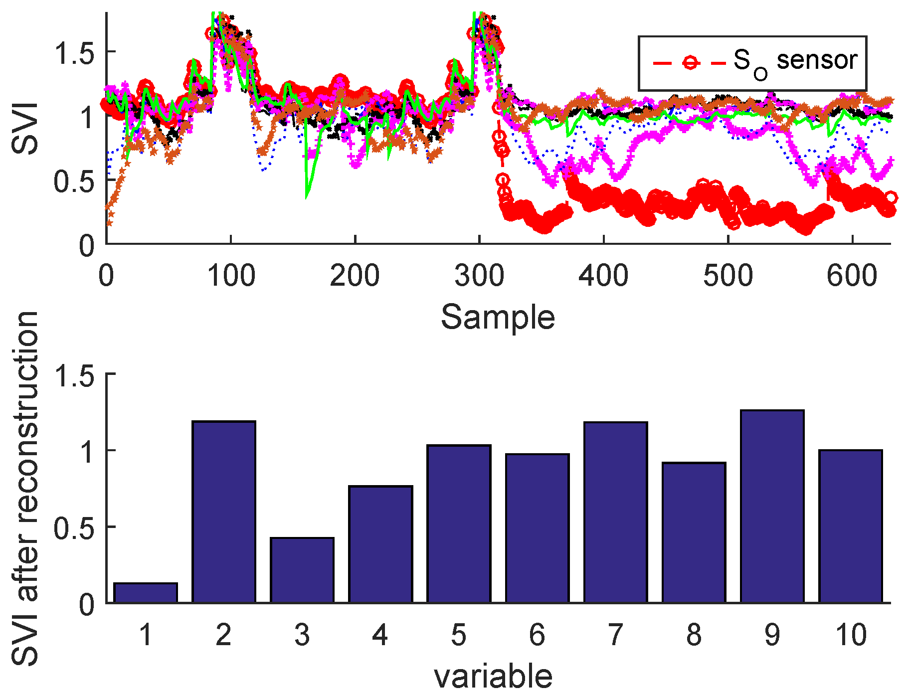
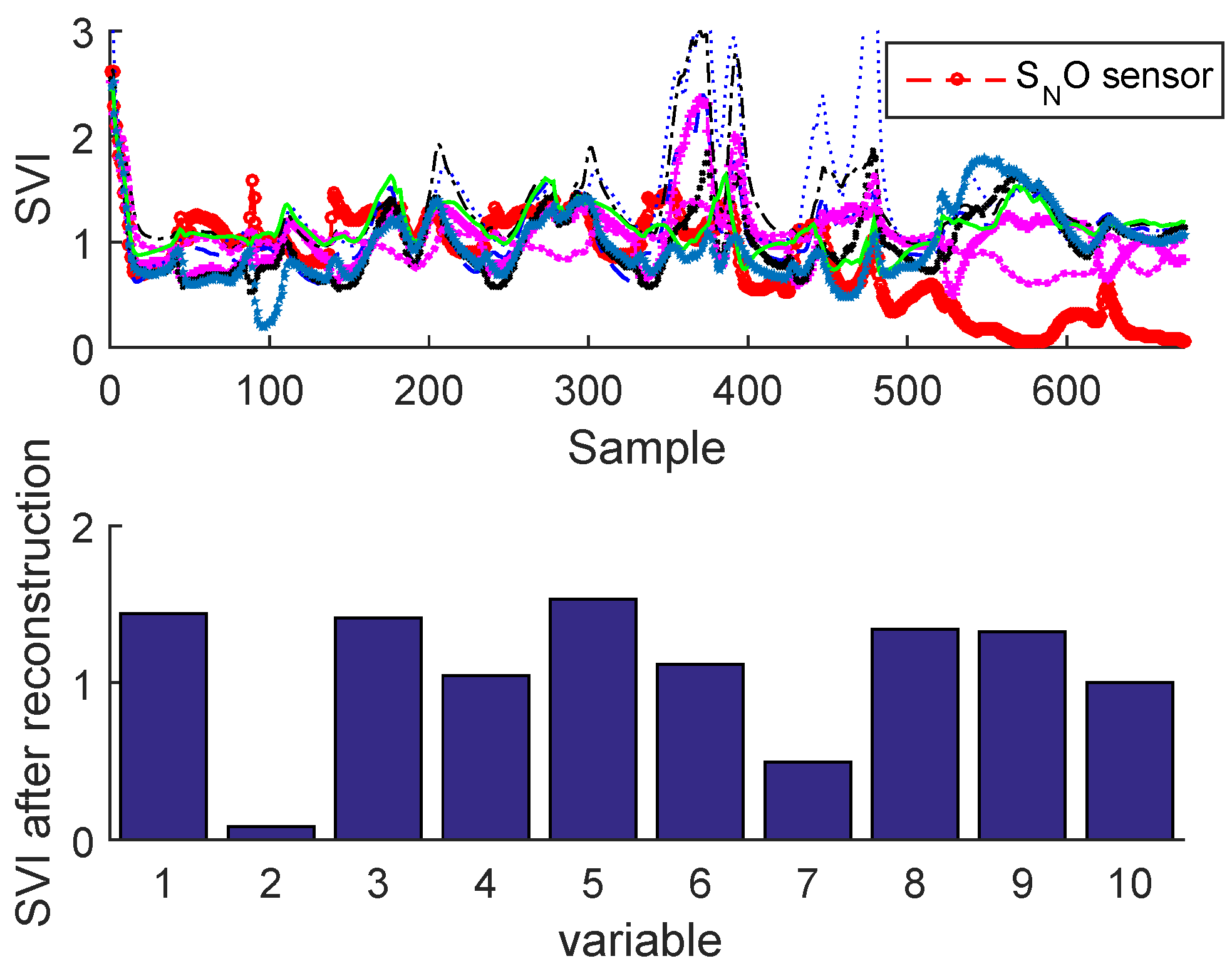
Figure 25 and Figure 26 illustrate the sensor validity indexes of BSM1 data and real data of all sensors after reconstruction for bias fault, and Figure 27 and Figure 28 for drift fault, in which the faults are eliminated by the correction of erroneous measure using the reconstruction principle. In this way, it is clear that the corrected sensor is faulty.
The SVIs can be immediately displayed on-line as soon as the abnormal event is detected. According to these SVIs which are not limited to isolating the faulty sensor, but can also show the correlation of the faulty sensor with other variables, in this way it can be seen that some sensors have been influenced by the reconstruction (as the sensor having the second largest contribution; see Figure 23 and Figure 24) due to high correlation with the faulty sensor. This can help the operator to provide a feasible interpretation. It should be noted that we can easily test any type of fault on any sensor, except the precision degradation fault is not localizable by the contribution plots or SVIs.
Finally, the comparative study shows that the proposed strategy has superior performance and is more effective for fault monitoring and diagnosis compared to the traditional methods like NLPCA or ICA, which are sensitive with the false alarms because of their constant confidence limit, and also are considered very late in fault detection.
4. Conclusions
The study described in this work concerns an enhanced control chart to monitor nonlinear processes and detect abnormal behaviours. The proposed strategy combines a Gaussian mixture model (GMM) with enhanced bottleneck neural networks (EBNN) to improve multivariate statistical process control (MSPC) using an adaptive upper control limit which is able to reduce the false alarms usually generated when the traditional upper control limit is used, since the proposed EBNN not only provides an estimated value of the input vector, but also probability rates of belonging to different operating modes. In addition, the filter applied to the SVI and SPE adds an important feature to minimize the number of false alarms.
To identify the faulty sensor, SVI based on the reconstruction error of the erroneous measure is successfully employed which gives a better diagnosis rate compared to the traditional contribution plots. However, the reconstruction allows the faulty sensor to be identified by comparing the sensor validity indexes before and after reconstructions of all measurements for each sensor—this can lead to the isolation of the faulty sensor.
Acknowledgments
The authors appreciate the valuable comments and suggestions of the reviewers. The authors would also like to thank the staff of the Annaba urban wastewater treatment plant, Algeria, for their time and help.
Author Contributions
Both authors contributed equally to the design, research and writing of the manuscript.
Conflicts of Interest
The authors declare no conflict of interest.
Abbreviations
The following abbreviations are used in this manuscript:
| PCA | Principal Component Analysis |
| ICA | Independent Component Analysis |
| BNN | Bottleneck Neural Network |
| EBNN | Enhanced Bottleneck Neural Network |
| GMM | Gaussian Mixture Model |
| KDE | Kernel Density Estimation |
| MSPC | Multivariate Statistical Process Control |
| SVI | Sensor Validity Index |
| AUCL | Adaptive Upper Control Limit |
| UCL | Upper Control Limit |
| SPE | Squared Prediction Error |
| AANN | Auto-Associative Neural Network |
| ANNC | Artificial Neural Network Classifier |
| IWA | International Water Association |
| EWMA | Exponentially Weighted Moving Average |
| WWTP | Wastewater Treatment Plant |
| BSM1 | Benchmark Simulation Model no. 1 |
| SPM | Statistical Process Monitoring |
| SPC | Statistical Process Control |
References
- Kresta, J.V.; MacGregor, J.F.; Marlin, T.E. Multivariate statistical monitoring of process operating performance. Can. J. Chem. Eng. 1991, 69, 35–47. [Google Scholar] [CrossRef]
- McAvoy, T.J.; Ye, N. Base Control for the Tennessee Eastman Problem. Comput. Chem. Eng. 1994, 18, 383–413. [Google Scholar] [CrossRef]
- Kourti, T.; MacGregor, J.F. Recent Developments in Multivariate SPC Methods for Monitoring and Diagnosing Process and Product Performance. J. Qual. Technol. 1996, 28, 409–428. [Google Scholar]
- Dunia, R.; Qin, S.J.; Edgar, T.F.; McAvoy, T.J. Use of principal component analysis for sensor fault identification. Comput. Chem. Eng. 1996, 20, S713–S718. [Google Scholar] [CrossRef]
- MacGregor, J.F.; Kourti, T.; Nomikos, P. Anlysis, Monitoring and fault diagnosis of industrial process using multivariate statistical projection methods. In Proceedings of the 13th Triennial Word Congress (IFAC), San Francisco, CA, USA, 30 June–5 July 1996; pp. 145–150. [Google Scholar]
- Wise, B.M.; Gallagher, N.B. The process chemometrics approach to process monitoring and fault detection. J. Process Control 1996, 6, 329–348. [Google Scholar] [CrossRef]
- Bakshi, B.R. Multiscale PCA with application to multivariate statistical process monitoring. AIChE J. 1998, 44, 1596–1610. [Google Scholar] [CrossRef]
- MacGregor, J.F.; Kourti, T. Statistical process control of multivariate processes. Control Eng. Pract. 1995, 3, 403–414. [Google Scholar] [CrossRef]
- Dunia, R.; Qin, S.J.; Edgar, T.F.; McAvoy, T.J. Identification of faulty sensors using principal component analysis. AIChE J. 1996, 42, 2797–2812. [Google Scholar] [CrossRef]
- Dong, D.; McAvoy, T.J. Nonlinear principal component analysis based on principal curves and neural networks. Comput. Chem. Eng. 1996, 20, 65–78. [Google Scholar] [CrossRef]
- Martin, E.B.; Morris, A.J.; Zhang, J. Process performance monitoring using multivariate statistical process control. IEE Proc.-Control Theory Appl. 1996, 143, 132–144. [Google Scholar] [CrossRef]
- Ge, Z.; Song, Z. Process monitoring based on independent component analysis—Principal component analysis (ICA-PCA) and similarity factors. Ind. Eng. Chem. Res. 2007, 46, 2054–2063. [Google Scholar] [CrossRef]
- Kramer, M.A. Nonlinear principal component analysis using autoassociative neural networks. AIChE J. 1991, 37, 233–243. [Google Scholar] [CrossRef]
- He, Q.P.; Wang, J. Fault Detection Using the k-Nearest Neighbor Rule for Semiconductor Manufacturing Processes. IEEE Trans. Semicond. Manuf. 2007, 20, 345–354. [Google Scholar] [CrossRef]
- Yu, H. A Just-in-time Learning Approach for Sewage Treatment Process Monitoring with Deterministic Disturbances. In Proceedings of the 2015-41st Annual Conference of the IEEE Industrial Electronics Society IECON, Yokohama, Japan, 9–12 November 2015; pp. 59–64. [Google Scholar]
- Dobos, L.; Abonyi, J. On-line detection of homogeneous operation ranges by dynamic principal component analysis based time-series segmentation. Chem. Eng. Sci. 2012, 75, 96–105. [Google Scholar] [CrossRef]
- Zhao, S.; Xu, Y. Multivariate statistical process monitoring using robust nonlinear principal component analysis. Tsinghua Sci. Technol. 2005, 10, 582–586. [Google Scholar]
- Verdier, G.; Ferreira, A. Fault detection with an adaptive distance for the k-nearest neighbors rule. Preoceedings of the IEEE International Conference on Computers and Industrial Engineering CIE, Troyes, France, 6–9 July 2009; pp. 1273–1278. [Google Scholar]
- Yu, J. A particle filter driven dynamic Gaussian mixture model approach for complex process monitoring and fault diagnosis. J. Process Control 2012, 22, 778–788. [Google Scholar] [CrossRef]
- Yu, J. A nonlinear kernel Gaussian mixture model based inferential monitoring approach for fault detection and diagnosis of chemical processes. Chem. Eng. Sci. 2012, 68, 506–519. [Google Scholar] [CrossRef]
- Figueiredo, M.A.T.; Jain, A.K. Unsupervised learning of finite mixture models. IEEE Trans. Pattern Anal. Mach. Intell. 2002, 24, 381–396. [Google Scholar] [CrossRef]
- Wang, G.; Cui, Y. On line tool wear monitoring based on auto associative neural network. J. Intell. Manuf. 2013, 24, 1085–1094. [Google Scholar] [CrossRef]
- Huang, Y. Advances in artificial neural networks methodological development and application. Algorithms 2009, 2, 973–1007. [Google Scholar] [CrossRef]
- Dev, A.; Krôse, B.J.A.; and Groen, F.C.A. Recovering patch parameters from the optic flow with associative neural networks. In Proceedings of the 1995 International Conference on Intelligent Autonomous Systems. Karlsruche, Germany, March 27–30; 1995; pp. 213–216. [Google Scholar]
- Jung, C.; Ban, S.W.; Jeong, S.; Lee, M. Input and output mapping sensitive auto-associative multilayer perceptron for computer interface system based on image processing of laser pointer spot. Neural Inf. Process. Models Appl. 2010. [Google Scholar] [CrossRef]
- Box, G.E.P. Some Theorems on Quadratic Forms Applied in the Study of Analysis of Variance Problems. Ann. Math. Stat. 1954, 25, 290–302. [Google Scholar] [CrossRef]
- Chen, T.; Morris, J.; Martin, E. Probability density estimation via an infinite Gaussian mixture model: Application to statistical process monitoring. J.R. Stat. Soc. Ser. C (Appl. Stat.) 2006, 55, 699–715. [Google Scholar] [CrossRef]
- Xiong, L.; Liang, J.; Jixin, Q. Multivariate Statistical Process Monitoring of an Industrial Polypropylene Catalyzer Reactor with Component Analysis and Kernel Density Estimation. Chin. J. Chem. Eng. 2007, 15, 524–532. [Google Scholar] [CrossRef]
- Odiowei, P.E.P.; Cao, Y. Nonlinear dynamic process monitoring using canonical variate analysis and kernel density estimations. IEEE Trans. Ind. Inform. 2010, 6, 36–45. [Google Scholar] [CrossRef]
- Chen, Q.; Wynne, R. J.; Goulding, P.; Sandoz, D. The application of principal component analysis and kernel density estimation to enhance process monitoring. Control Eng. Pract. 2000, 8, 531–543. [Google Scholar] [CrossRef]
- Liang, J. Multivariate statistical process monitoring using kernel density estimation. Dev. Chem. Eng. Min. Process. 2005, 13, 185–192. [Google Scholar] [CrossRef]
- Harkat, M.F.; Mourot, G.; Ragot, J. An improved PCA scheme for sensor FDI: Application to an air quality monitoring network. J. Process Control 2006, 16, 625–634. [Google Scholar] [CrossRef]
- Bouzenad, K.; Ramdani, M.; Zermi, N.; Mendaci, K. Use of NLPCA for sensors fault detection and localization applied at WTP. In Proceedings of the 2013 World Congress on Computer and Information Technology (WCCIT), Sousse, Tunisia, 22–24 June 2013; pp. 1–6. [Google Scholar]
- Bouzenad, K.; Ramdani, M.; Chaouch, A. Sensor fault detection, localization and reconstruction applied at WWTP. In Proceedings of the 2013 Conference on Control and Fault-Tolerant Systems (SysTol), Nice, France, 9–11 October 2013; pp. 281–287. [Google Scholar]
- Chaouch, A.; Bouzenad, K.; Ramdani, M. Enhanced Multivariate Process Monitoring for Biological Wastewater Treatment Plants. Int. J. Electr. Energy 2014, 2, 131–137. [Google Scholar] [CrossRef]
- Carnero, M.; HernÁndez, J.L.; SÁnchez, M.C. Design of Sensor Networks for Chemical Plants Based on Meta-Heuristics. Algorithms 2009, 2, 259–281. [Google Scholar] [CrossRef]
- Zhao, W.; Bhushan, A.; Santamaria, A.D.; Simon, M.G.; Davis, C.E. Machine learning: A crucial tool for sensor design. Algorithms 2008, 1, 130–152. [Google Scholar] [CrossRef] [PubMed]
- Aguado, D.; Rosen, C. Multivariate statistical monitoring of continuous wastewater treatment plants. Eng. Appl. Artif. Intell. 2008, 21, 1080–1091. [Google Scholar] [CrossRef]
- Rosen, C.; Olsson, G. Disturbance detection in wastewater treatment plants. Water Sci. Technol. 1998, 37, 197–205. [Google Scholar] [CrossRef]
- Zhao, L.J.; Chai, T.Y.; Cong, Q.M. Multivariate statistical modeling and monitoring of SBR wastewater treatment using double moving window PCA. Mach. Learn. Cybern. 2004, 3, 1371–1376. [Google Scholar]
- Alex, J.; Benedetti, L.; Copp, J.; Gernaey, K.V.; Jeppsson, U.; Nopens, I.; Pons, M.N.; Rieger, L.; Rosen, C.; Steyer, J. Benchmark Simulation Model no. 1 (BSM1.). 2008. Available online: http://www.iea.lth.se/publications/Reports/LTH-IEA-7229.pdf (accessed on 28 April 2017).
- Yoo, C.K.; Villez, K.; Lee, I.B.; Van Hulle, S.; Vanrolleghem, P.A. Sensor validation and reconciliation for a partial nitrification process. Water Sci. Technol. 2006, 53, 513–521. [Google Scholar] [CrossRef] [PubMed]
- Yoo, C.K.; Villez, K.; Van Hulle, S.W.; Vanrolleghem, P.A. Enhanced process monitoring for wastewater treatment systems. Environmetrics 2008, 19, 602–617. [Google Scholar] [CrossRef]
Figure 1.
Process monitoring cycle.

Figure 2.
EBNN for variables estimation and modes classification.

Figure 3.
Reconstruction principle.
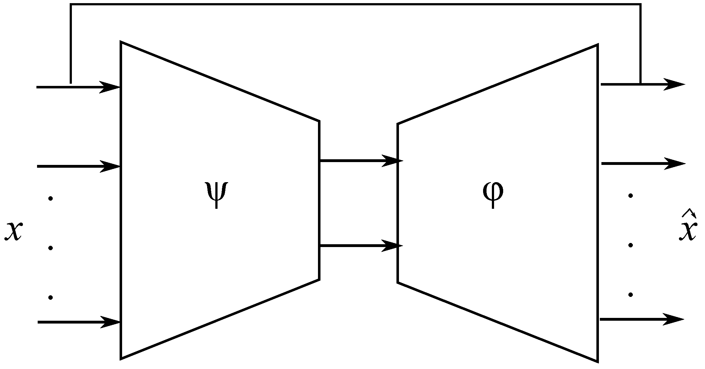
Figure 4.
General overview of the benchmark simulation model no. 1 (BSM1) plant.
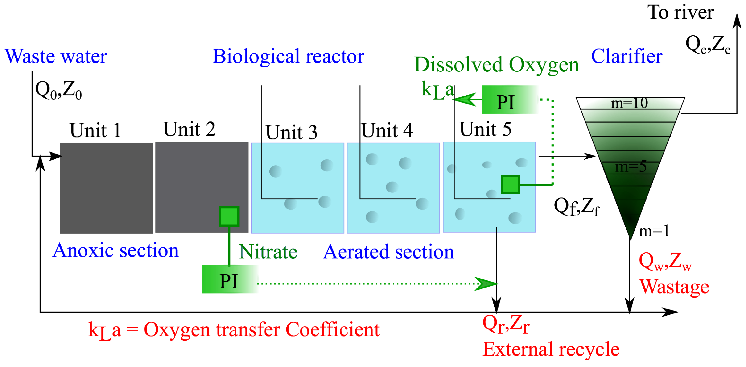
Figure 5.
Simulink of BSM1.

Figure 6.
Schematic of Annaba wastewater treatment plant.
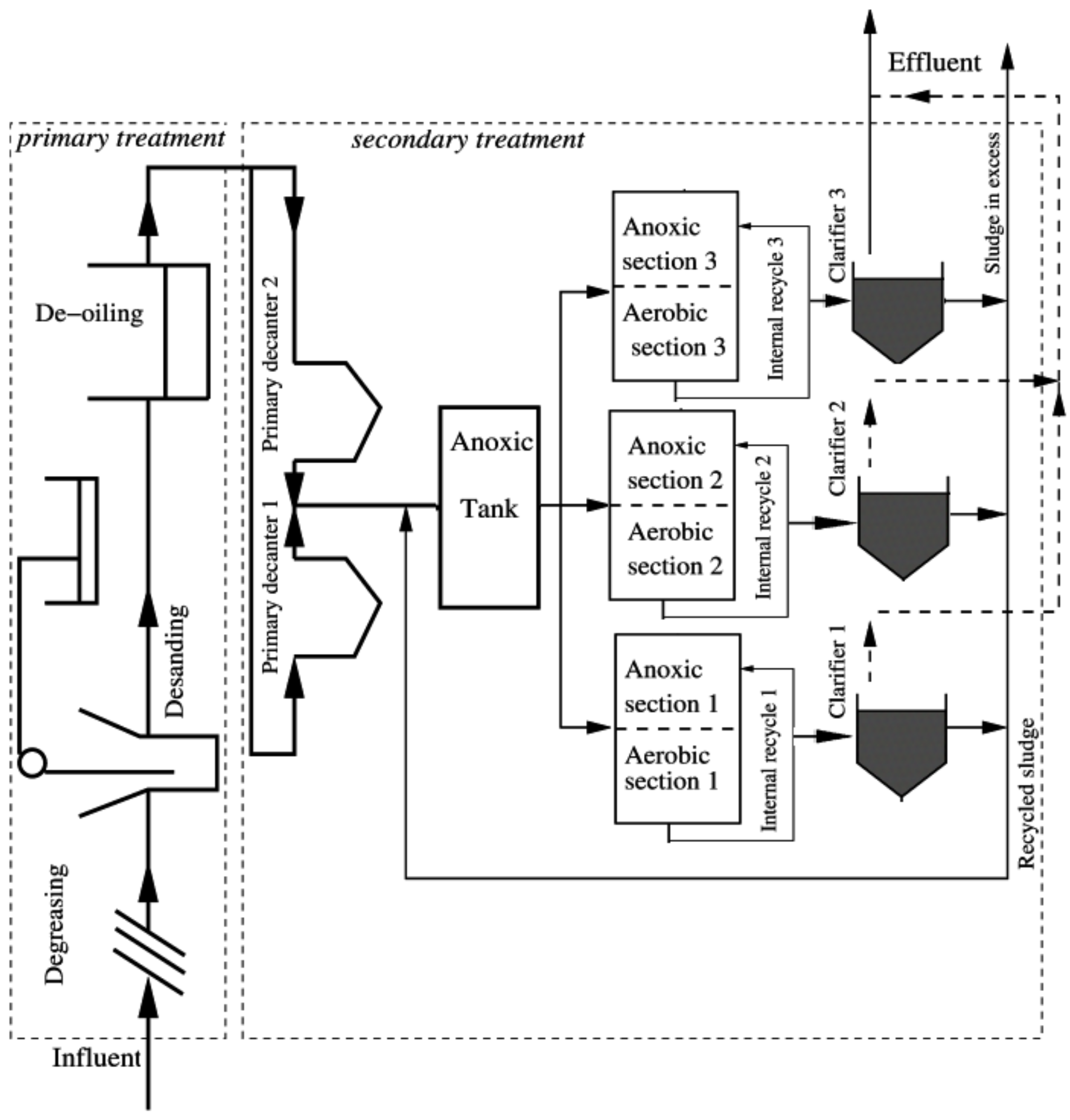
Figure 7.
Squared prediction error (SPE) during normal operating state (no fault) using independent component analysis (ICA) for the BSM1 data.
Figure 7.
Squared prediction error (SPE) during normal operating state (no fault) using independent component analysis (ICA) for the BSM1 data.
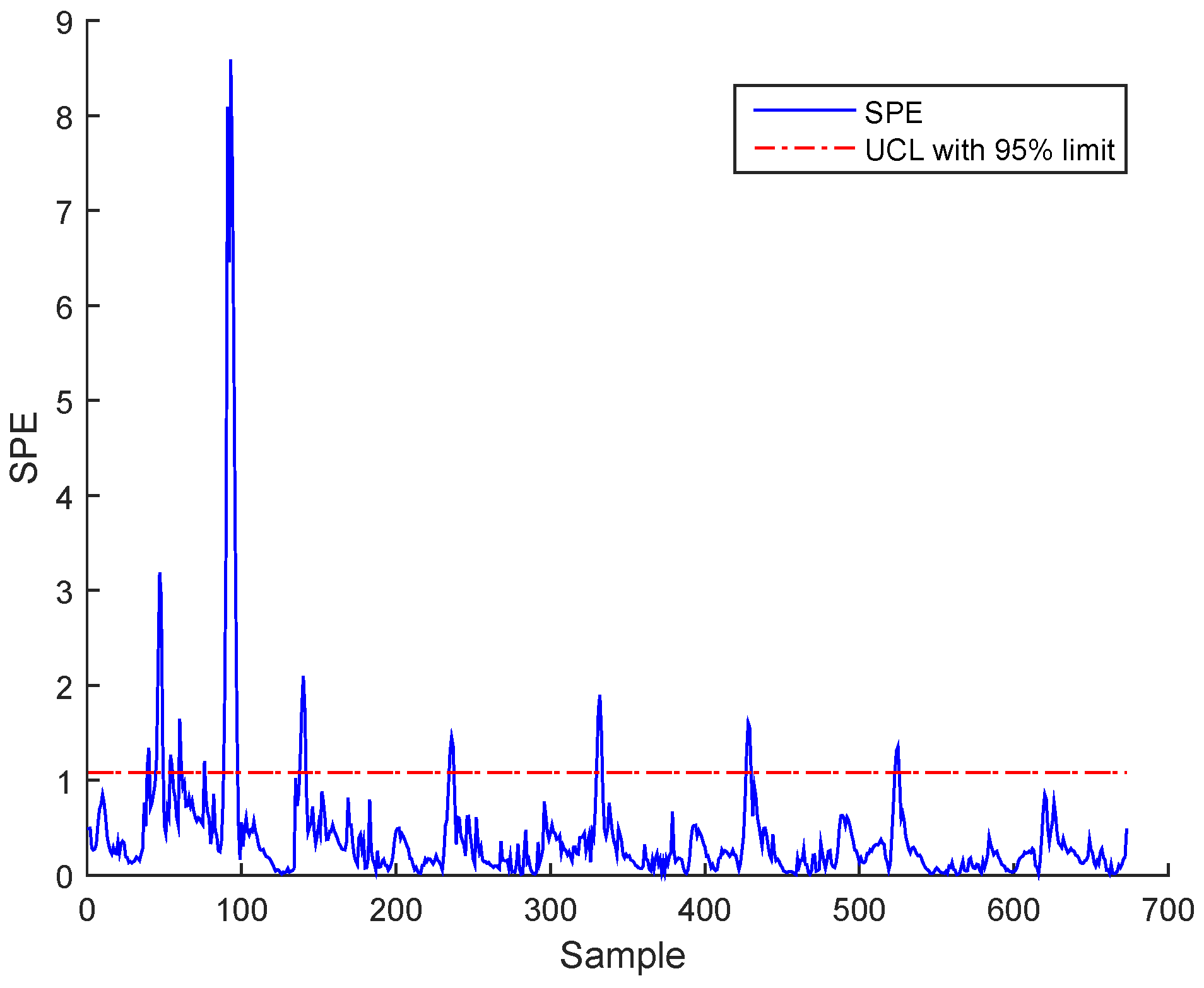
Figure 8.
SPE during normal operating state (no fault) using ICA for real data.

Figure 9.
SPE during normal operating state (no fault) using ICA for the BSM1 data.
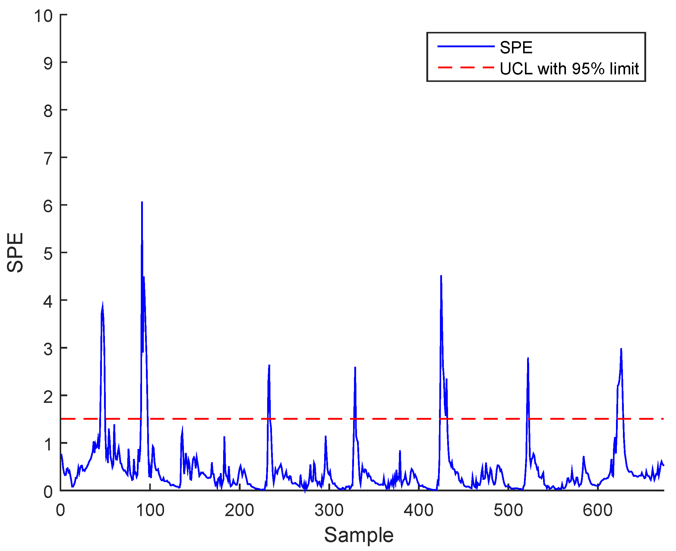
Figure 10.
SPE during normal operating state (no fault) with nonlinear principal component analysis (NLPCA) for the actual wastewater treatment plant (WWTP) data.
Figure 10.
SPE during normal operating state (no fault) with nonlinear principal component analysis (NLPCA) for the actual wastewater treatment plant (WWTP) data.

Figure 11.
Evolution of , and after normalization and their estimations of BSM1 data.
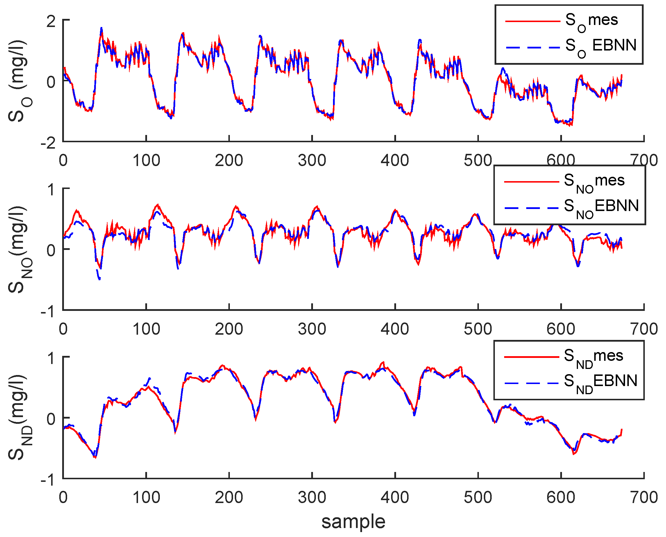
Figure 12.
Evolution of , and after normalization and their estimations of real data.

Figure 13.
Probability rates of various operating modes of BSM1 data.

Figure 14.
Probability rates of various operating modes of real data.
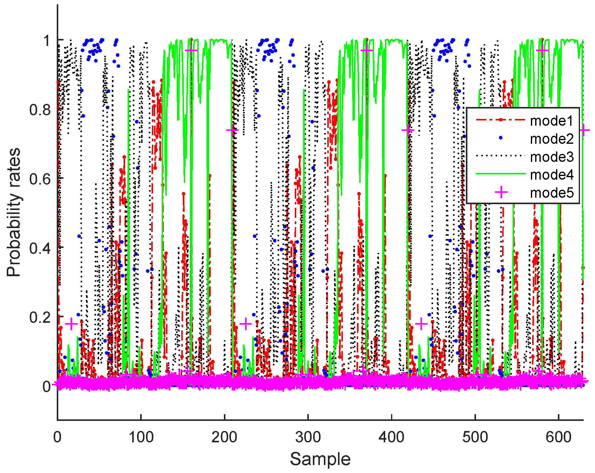
Figure 15.
Filtered SPE during normal operating state (no fault) with an adaptive upper control limit (AUCL) based on kernel density estimation (KDE) of BSM1 data.
Figure 15.
Filtered SPE during normal operating state (no fault) with an adaptive upper control limit (AUCL) based on kernel density estimation (KDE) of BSM1 data.

Figure 16.
Filtered SPE during normal operating state (no fault) with an adaptive UCL based on KDE of real data.
Figure 16.
Filtered SPE during normal operating state (no fault) with an adaptive UCL based on KDE of real data.

Figure 17.
Filtered SPE for precision degradation fault in sensor of BSM1.

Figure 18.
Filtered SPE for precision degradation fault in sensor of real data.

Figure 19.
Filtered SPE for bias fault in sensor sensor of the BSM1 data.

Figure 20.
Filtered SPE for bias fault in sensor sensor of the real data.

Figure 21.
Filtered SPE for drift fault in sensor sensor of the BSM1 data.
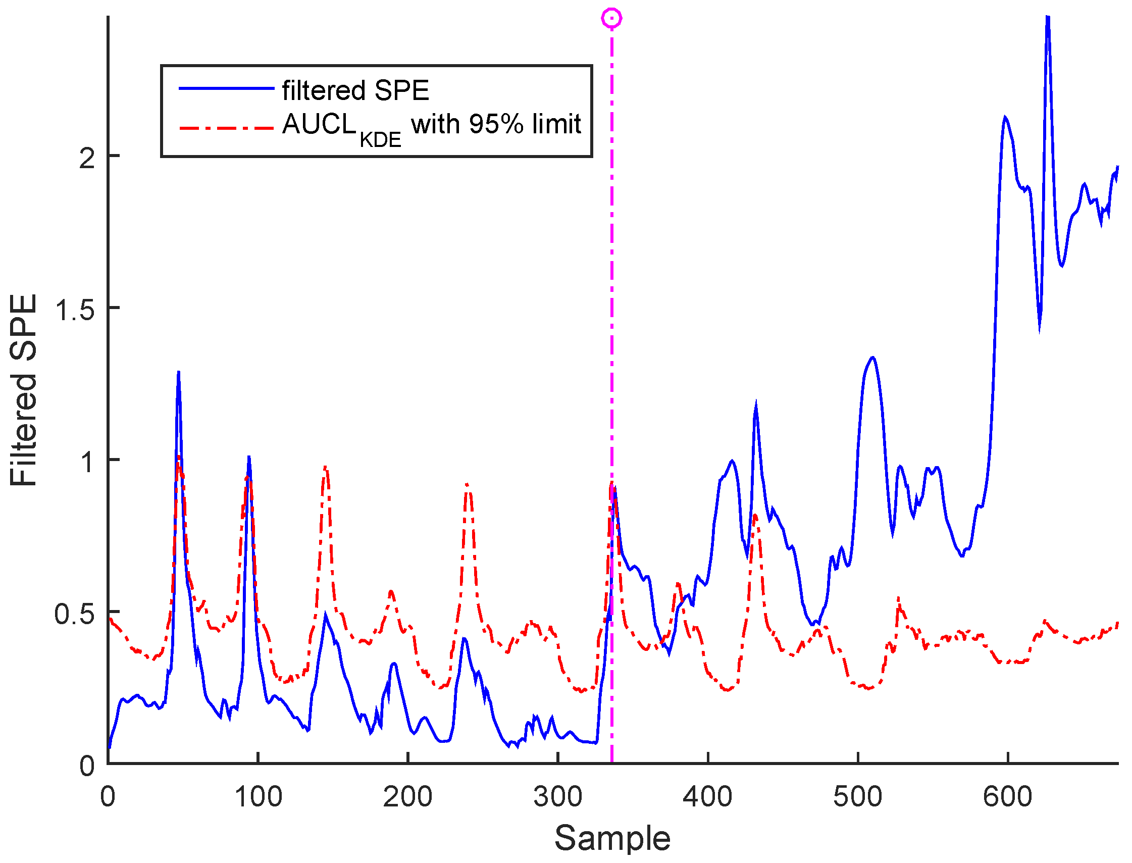
Figure 22.
Filtered SPE for drift fault in sensor sensor of the real data.
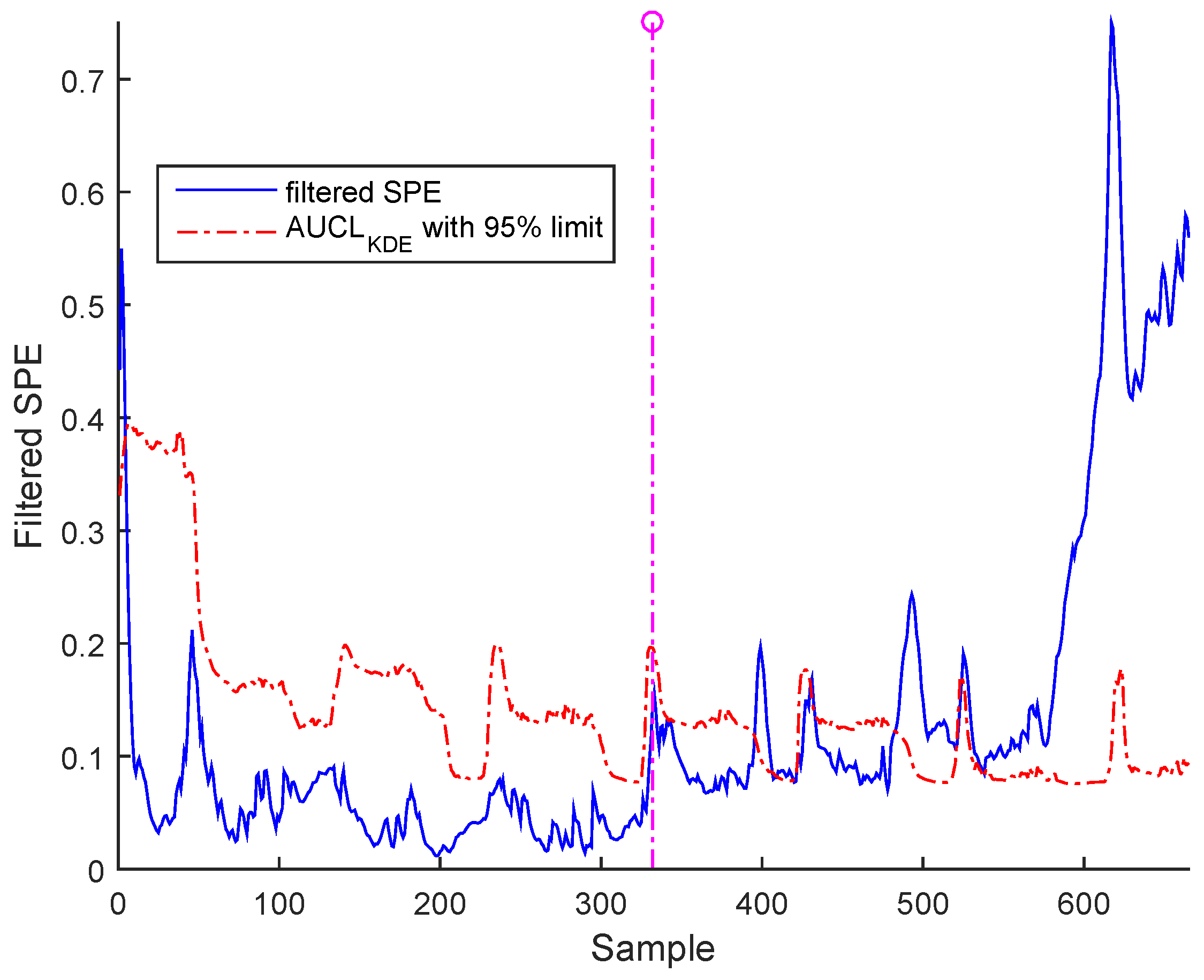
Figure 23.
Fault isolation by contribution plots for drift fault of BSM1 data (Sensor S).

Figure 24.
Fault isolation by contribution plots for drift fault of real data (Sensor S).
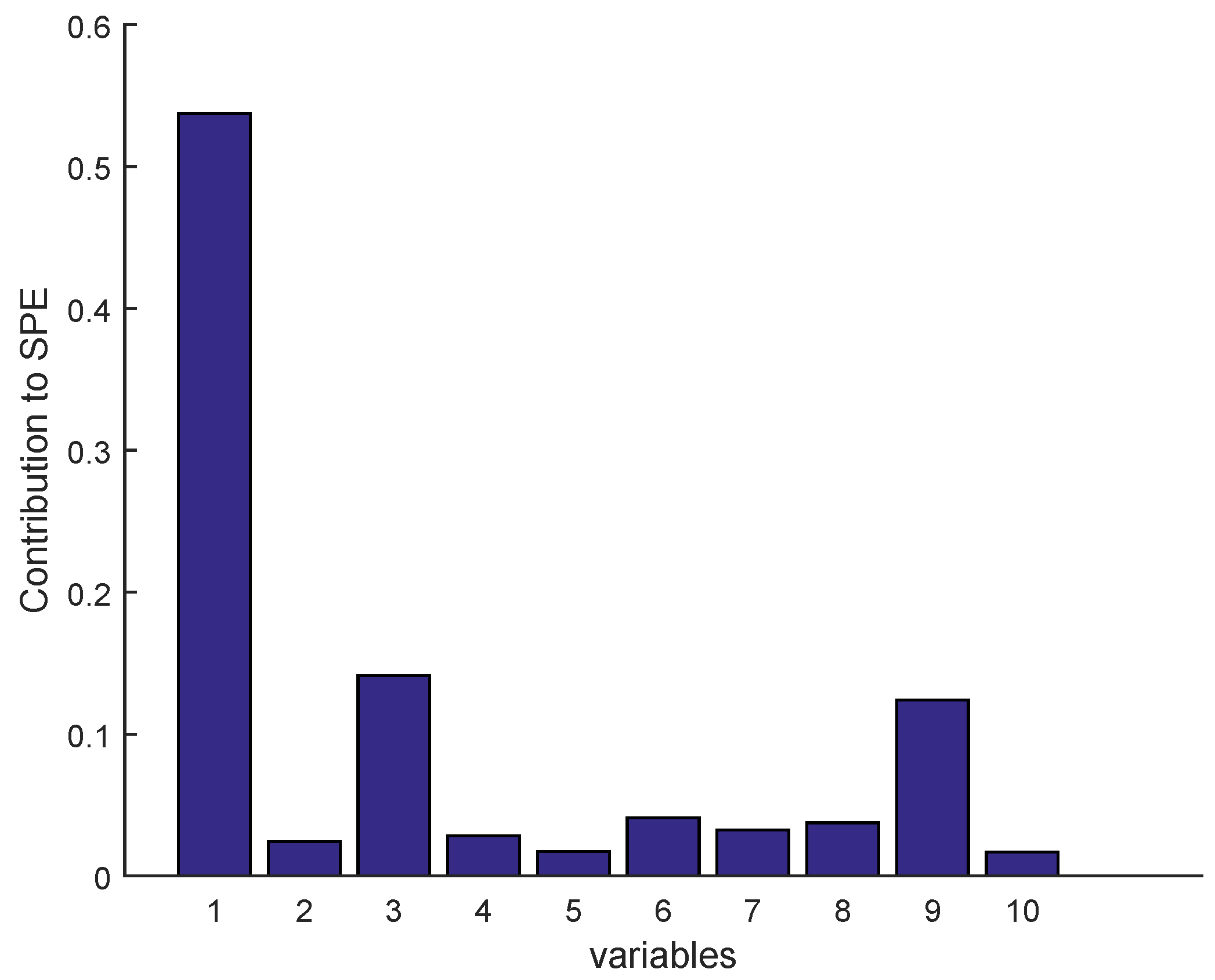
Figure 25.
Fault isolation by sensor validity indexes for bias fault of BSM1 data.
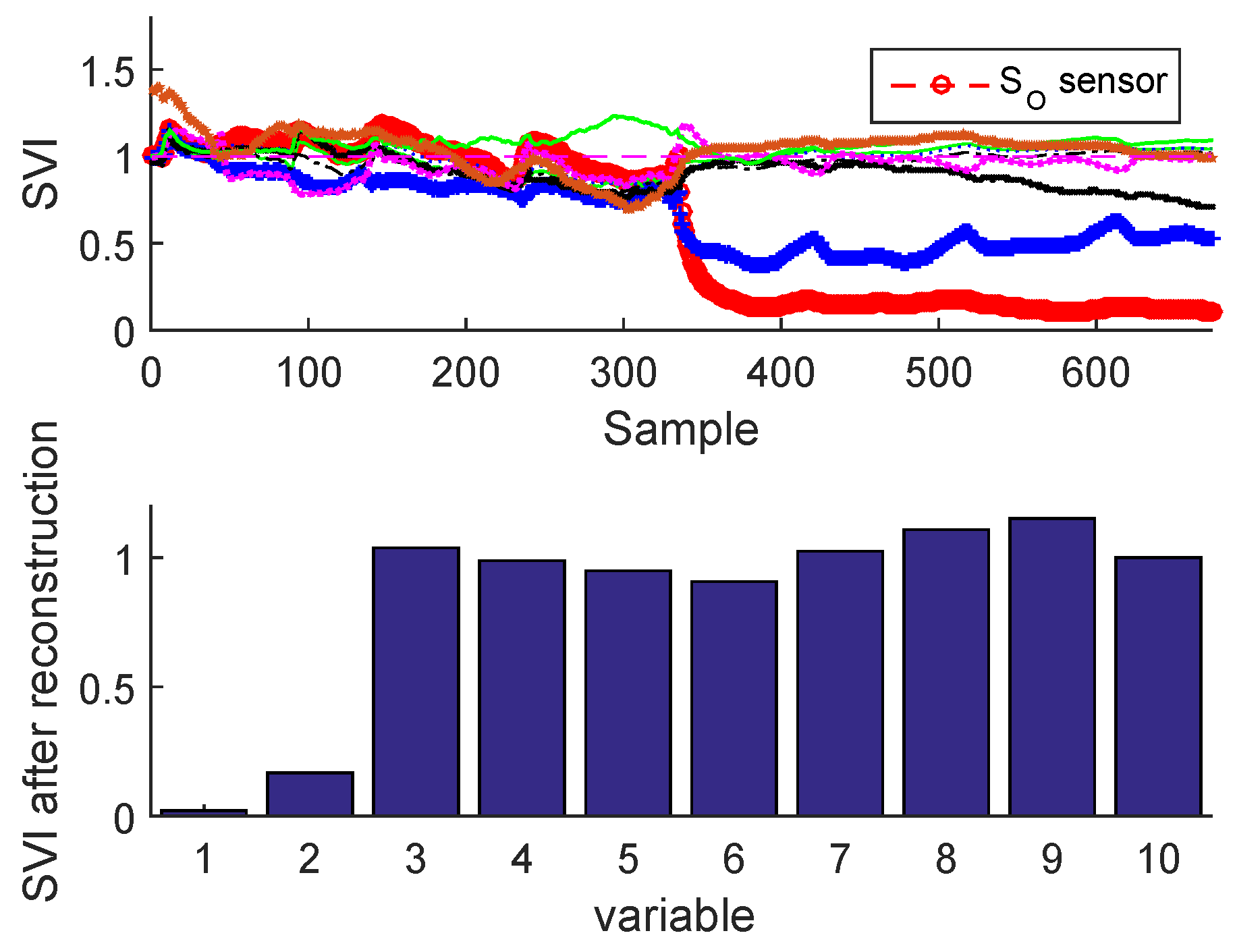
Figure 26.
Fault isolation by sensor validity indexes for bias fault of real data.

Figure 27.
Fault isolation by sensor validity indexes for drift fault of BSM1 data.
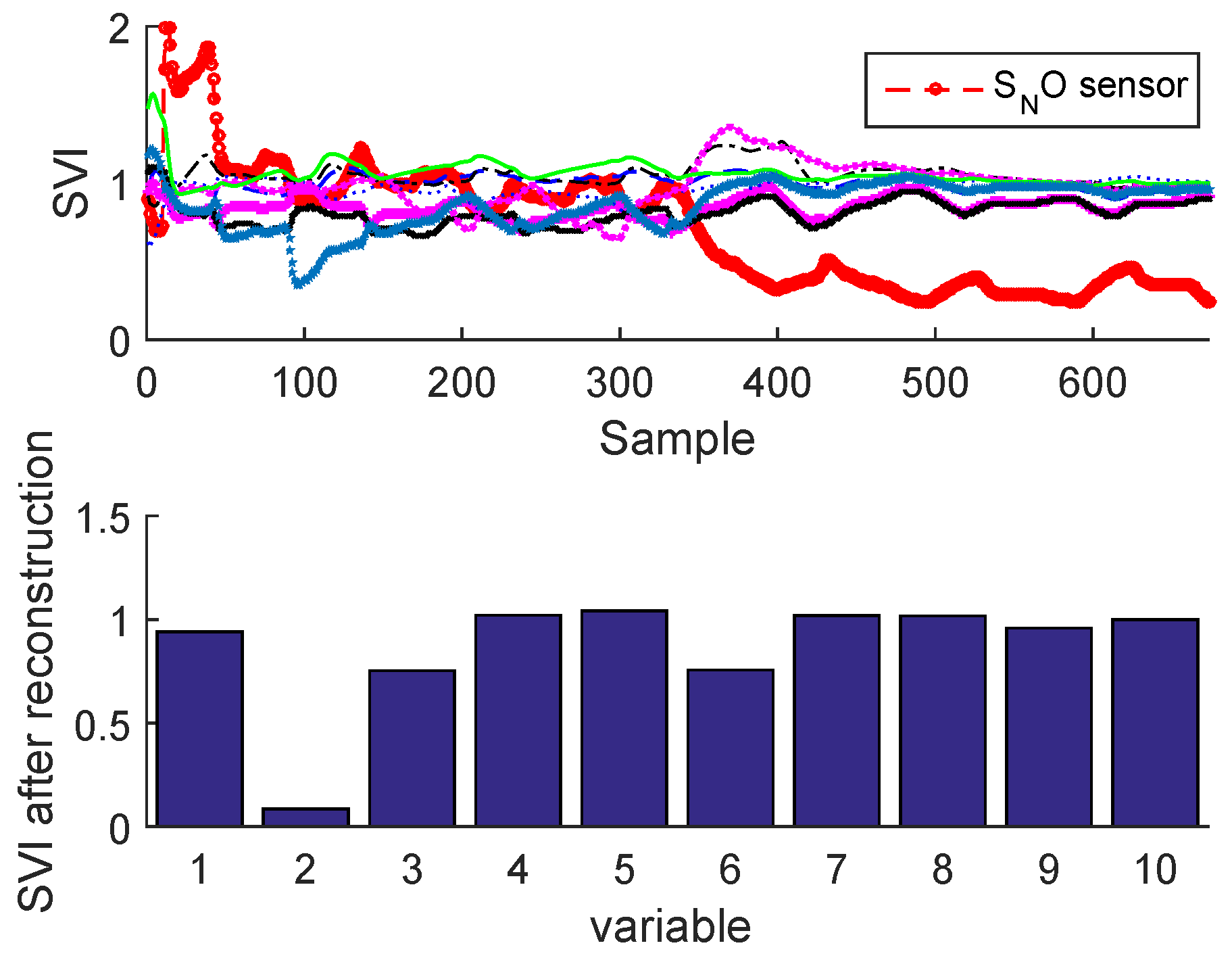
Figure 28.
Fault isolation by sensor validity indexes for drift fault of real data.


Table 1.
The monitored sensors for BSM1 plant.
| N | Monitored Sensors | Notation |
|---|---|---|
| 1 | Dissolved oxygen in | |
| 2 | Nitrate and nitrite nitrogen in | |
| 3 | nitrogen in | |
| 4 | Soluble biodegradable organic nitrogen in | |
| 5 | Particulate biodegradable organic nitrogen in | |
| 6 | Dissolved oxygen in | |
| 7 | Nitrate and nitrite nitrogen in | |
| 8 | nitrogen in | |
| 9 | Soluble biodegradable organic nitrogen in | |
| 10 | Particulate biodegradable organic nitrogen in |
Table 2.
The monitored sensors for the real process.
| N | Monitored Sensors | Notation |
|---|---|---|
| 1 | Dissolved oxygen in influent | |
| 2 | Nitrites in influent | |
| 3 | Nitrates in influent | |
| 4 | Ammoniacal nitrogen in influent | |
| 5 | Chemical oxygen demand in influent | |
| 6 | Dissolved oxygen in effluent | |
| 7 | Nitrites in effluent | |
| 8 | Nitrates in effluent | |
| 9 | Ammoniacal nitrogen in effluent | |
| 10 | Chemical oxygen demand in effluent |
Table 3.
Summary of fault scenarios.
| Fault type | Precision degradation | Bias | Drift |
|---|---|---|---|
| Fault expression | . | ||
| Faulty sensor expression | |||
| Fault time | 336 | 366 | 366 |
| 2*Detection time | 349.4 for BSM1 data and | 336.7 for BSM1 data and | 342.3 for BSM1 data and |
| 346.2 for real data | 337.2 for real data | 392.1 for real data |
© 2017 by the authors. Licensee MDPI, Basel, Switzerland. This article is an open access article distributed under the terms and conditions of the Creative Commons Attribution (CC BY) license (http://creativecommons.org/licenses/by/4.0/).
Share and Cite
MDPI and ACS Style
Bouzenad, K.; Ramdani, M. Multivariate Statistical Process Control Using Enhanced Bottleneck Neural Network. Algorithms 2017, 10, 49. https://doi.org/10.3390/a10020049
AMA Style
Bouzenad K, Ramdani M. Multivariate Statistical Process Control Using Enhanced Bottleneck Neural Network. Algorithms. 2017; 10(2):49. https://doi.org/10.3390/a10020049
Chicago/Turabian StyleBouzenad, Khaled, and Messaoud Ramdani. 2017. "Multivariate Statistical Process Control Using Enhanced Bottleneck Neural Network" Algorithms 10, no. 2: 49. https://doi.org/10.3390/a10020049
Note that from the first issue of 2016, this journal uses article numbers instead of page numbers. See further details here.