Intelligent Dynamic Backlash Agent: A Trading Strategy Based on the Directional Change Framework
by
Amer Bakhach
1,*, 
Venkata L. Raju Chinthalapati
2,
Edward P. K. Tsang
1 and
Abdul Rahman El Sayed
3 1
Centre for Computational Finance and Economic Agents, University of Essex, Colchester CO4 3SQ, UK
2
Department of Accounting and Finance, University of Greenwich, London SE10 9LS, UK
3
Department of Mathematics, Normandie University, 76620 Normandie, France
*
Author to whom correspondence should be addressed.
Algorithms 2018, 11(11), 171; https://doi.org/10.3390/a11110171
Submission received: 17 September 2018
/
Revised: 22 October 2018
/
Accepted: 26 October 2018
/
Published: 28 October 2018
(This article belongs to the Special Issue Algorithms in Computational Finance)
Abstract
:The Directional Changes (DC) framework is an approach to summarize price movement in financial time series. Some studies have tried to develop trading strategies based on the DC framework. Dynamic Backlash Agent (DBA) is a trading strategy that has been developed based on the DC framework. Despite the promising results of DBA, DBA employed neither an order size management nor risk management components. In this paper, we present an improved version of DBA named Intelligent DBA (IDBA). IDBA overcomes the weaknesses of DBA as it embraces an original order size management and risk management modules. We examine the performance of IDBA in the forex market. The results suggest that IDBA can provide significantly greater returns than DBA. The results also show that the IDBA outperforms another DC-based trading strategy and that it can generate annualized returns of about 30% after deducting the bid and ask spread (but not the transaction costs).
1. Introduction
Directional Change (DC) is an approach to summarizing market price movements [1]. Under the DC framework, the market is cast into alternating upward trends, which we call uptrend, and downward trends, which we call downtrend [2]. A trend is identified as a change in market price larger than, or equal to, a given threshold. This threshold, named is set by the observer and usually expressed as percentage. A trend ends whenever a price change of the same threshold, , is observed in the opposite direction. For example, a market downtrend ends when we observe a price rise of magnitude ; in this case, we say that the market changes its direction to an uptrend. Similarly, a market’s uptrend ends when we observe a price decline of magnitude , in which case we say that the market changes its direction to a downtrend.
Before we continue, we cite other studies that show the DC framework has helped in analyzing financial markets. For example, Glattfelder et al. [3] discovered twelve scaling laws which unveil new characteristics in the Forex (FX) market. These scaling laws are based on the DC concept. They aimed to establish mathematical relationships among price moves, duration and frequency. In addition, Bisig et al. [4] presented the so-called Scale of Market Quakes (SMQ) based on the DC concept. SMQ aims to quantify FX market activity during significant economic and political events declarations.
Furthermore, Masry [5] reported a study that deciphers FX market activity based on the DC concept. She introduced an approach that lays “the foundations for understanding how FX market activity changes as the price movement progresses” and explains how minor differences in market activities can change the price trend, under definite conditions, during the overshoot (OS) event [5]. Bakhach et al. [6] presented a model to forecast market trend’s direction under the DC framework. They tried to forecast whether a DC trend would continue for a specific threshold before the market’s trend reverses. AlKhamees and Fasli [7] proposed a DC-based approach with a dynamic threshold definition method to analyze the reaction of financial market to the published news (e.g., political, economic). They claimed that their approach can be used by investors to detect movements in the market so that they can, potentially, react to and take advantage of.
Tsang et al. [8] introduced an approach to profiling companies and financial markets. Their methodology embraces a set of innovative indicators that are based on the DC framework. These indicators aim to analyze and classify financial markets. They concluded that information obtained through DC-based analysis and from time series complement each other. Tsang and Chen [9] suggested an approach to profile a particular market over a rolling time window, and track the change of market positions over time. They employed some of the DC indicators previously introduced in [8] observed under different price events. They applied their approach to identify regime change during the Brexit period (more particularly between May and July 2016).
In addition, some studies have tried to develop trading strategies based on the DC framework (e.g., [10,11,12,13]). In this paper, we are particularly interested in the DC-based trading strategy named Dynamic Backlash Agent (DBA) by Bakhach et al. [14]. The preliminary results suggest that DBA can generate positive returns in many cases. However, DBA has two critical weaknesses: (a) it does not have any order size management; and (b) it does not have any risk management module. In this paper we introduce an improved version of DBA called Intelligent DBA (IDBA). IDBA is designed to overcome these two weaknesses of DBA.
This paper continues as follows: Section 2 describes the concept of Directional Changes. Section 3 provides a brief review of the existing trading strategies that are based on the DC framework. Section 4 provides a summary of the trading strategy named DBA. We present the components of IDBA and explain how it functions in Section 5. We discuss the selection and preparation of the datasets in Section 6. The details of the experiments, conducted to evaluate the performance of IDBA, are provided in Section 7. Section 8 reports and discusses the results of these experiments. Finally, we summarize the major findings of this paper in Section 9.
2. Directional Changes: An Introduction
In this section, we explain how market prices are summarized based on the DC concept. Under the DC framework, the market is represented as alternating uptrends and downtrends. The basic idea is that the magnitude of price change during an uptrend, or a downtrend, must be at least equal to a specific threshold . Here, is a percentage that the observer considers substantial (usually expressed as a percentage). For example, Figure 1 depicts a price’s drop between points A and A0.1. This price drop is equal to the selected, hypothetical, threshold of 0.1%. In this case, we say that we have a DC downtrend that starts at point A. Any price change less than the identified threshold, , will not be considered as a trend when summarizing price movements [1,2]. Under the DC framework, each uptrend is followed by a downtrend and vice versa. The detection of a new uptrend, or downtrend, is a crucial task. The detection of a new downtrend, or uptrend, is a two-step algorithmic approach:
- Step 1: If the market is currently in a downtrend, let denotes the lowest price in this downtrend. The value of may change as the price movement continues. We use Table 1 to exemplify this note. For example, at time 20:55:00, in Table 1, the mid-price is 1.48260. The lowest price observed between time 20:55:00 and 20:58:00 is 1.48230 which was observed at time 20:56:00. Therefore, the value of , at time 20:58:00 is 1.48230. However, as the price’s movement continues, at time 21:01:00, the mid-price becomes 1.48180. In this case, the lowest price observed between point time 20:55:00 and time 21:01:00 becomes 1.48150 (which was observed at time 21:00:00). Similarly, if the market is currently in uptrend, then would refer to the highest price in this uptrend.
- Step 2: Let be the current price. We say that the market switches its direction from a downtrend to an uptrend if becomes greater than by at least (where is the threshold predetermined by the observer). Similarly, we say that the market switches its direction from an uptrend to a downtrend if becomes less than by at least . The detection of a new DC uptrend or a new DC downtrend is a formalized inequality, as shown in Equation (1). For example, in Table 1, at time 21:05:00, the current price, , is 1.48310. At time 21:05:00, the is 1.48150 (which was observed at time 21:00:00). In this case, the magnitude of price’s change between and is 0.1%. Thus, the inequality in Equation (1) holds and we can confirm the observation of a new DC uptrend. In other words, at time 21:05:00, we can confirm the observation of a new DC uptrend which has started at time 21:00:00. If the inequality in Equation (1) holds, then the time at which the market traded at is called an “extreme point” (e.g., point B in Table 1) and the time at which the market trades at is called a DC confirmation point, or DCC point for short (e.g., point B0.1 in Table 1). By definition, the extreme point of an uptrend has the lowest price amongst all points of current uptrend and the immediately preceding downtrend. Similarly, the extreme point of a downtrend has the highest price amongst all points of current downtrend and the immediately preceding uptrend.
Figure 2 illustrates the identification of extreme and DCC points for a given financial time series. In Figure 2, points A, B, C, D, E, F and G are the “extreme points”, whereas points A0.1, B0.1, C0.1, D0.1, E0.1, F0.1, and G0.1 are the “DCC points”. An extreme point can be seen as a local minimum (e.g., point D in Figure 2) or a local maximum (e.g., point C in Figure 2). An extreme point is only recognized in hindsight-precisely at the DCC point (i.e., when the inequality in Equation (1) becomes true). For example, in Figure 2, at point A0.1, we confirm that point A is an extreme point. Similarly, in Figure 2, at point D0.1, we confirm that point D is an extreme point. We denote by “price extreme” () the price at which a trend starts. Eventually, when Equation (1) holds, i.e., when a new DC trend is recognized (either uptrend or downtrend), the becomes the of this new DC trend.
Under the DC framework, a trend is dissected into a DC event and an overshoot (OS) event. A DC event starts with an extreme point and ends with a DCC point. We refer to a specific DC event by its starting point, i.e., extreme point, and its DCC point. For example, in Figure 2, the DC event which starts at point A and ends at point A0.1 is denoted as [AA0.1]. An OS event starts at the DCC point and ends at the next extreme point.
2.1. The DC Summary
The DC summary of a given market is the identification of the DC and OS events, governed by the threshold . Figure 2 shows an example of a DC summary with 0.1%. Note that we can produce multiple DC summaries for the same considered price series by selecting multiple thresholds. For example, Figure 2 and Figure 3 illustrate two distinct DC summaries for the same price series using two thresholds: 0.1% for Figure 2 and 0.2% for Figure 3.
Keep in mind that the observer should specify the value of the DC threshold . One observer may consider 0.1% to be an important change, while another observer may consider 0.2% as important. The chosen threshold determines what constitutes a directional change [2,3]. If a greater threshold had been chosen, then fewer directional changes would have been concluded between the points. For instance, in Figure 2, the DC summary of threshold 0.1% uncovers four downtrends and three uptrends, whereas, in Figure 3, the DC summary of threshold 0.2% uncovers two downtrends and one uptrend.
2.2. DC Notations
In this section, we introduce some basic notations related to the DC concept. These notations were initially introduced in Tsang et al. [8] and reshaped to fit with the context of this paper.
- -
- : This denotes the current price.
- -
- Extreme point: This is the point at which the current DC event starts.
- -
- It is the price at the extreme point of the current DC event. In the case of a downward DC event, refers to the highest price in this trend. In the case of an upward DC event, refers to the lowest price in this trend.
- -
- : If the market is in a downtrend (uptrend), then would refer to the lowest (highest) price in this downtrend (uptrend).
- -
- and The interpretations of these two variables depend on whether the market is in uptrend or downtrend:
- ○
- If the market is in uptrend, then would denote the minimum price required to confirm the current uptrend (see Equation (3)). If the market is in downtrend, then would denote the minimum price required to confirm the next downtrend.
- ○
- If the market is in downtrend, then would denote the highest price required to confirm the current downtrend (see Equation (2)). If the market is in downtrend, then would denote the highest price required to confirm the next uptrend.
- -
- : If the market is currently in downtrend, then we have = ; otherwise, = . In the case of downtrend, we compute as:otherwise:
- -
- : The objective of Overshoot Value (OSV) is to measure the magnitude of an overshoot event. Instead of using the absolute value of the price change, we would like this measure to be relative to the threshold, . OSV was initially formalized by Tsang et al. [8] as:
More details and examples regarding as to how to compute and are provided below.
3. Related Works
In this section, we review some existing DC-based trading strategies. However, firstly, we list and explain some common evaluation metrics that are usually employed to evaluate the performance of a trading strategy.
3.1. Evaluation Metrics
Many studies define success solely based on returns and win ratios, which, practically, has little value [15,16]. In fact, an investor might be interested in other metrics that evaluate the risk and risk-adjusted performance of a given trading strategy [17,18]. In this section, we explain a range of evaluation metrics that were marked as adequate for a decent evaluation of the performance of a given trading model [17,19].
- Rate of return: The rate of return (RR) symbolizes the bottom line for a trading system over a definite period. Total Profit (TP) represents the profitability of total trades. TP is computed by removing the sum of all losing trades from the sum of all winning trades (Equation (5)). TP can be negative when the loss is greater than the gain. We denote by RR (Equation (6)) the gain or loss on an investment over a given evaluation period expressed as a percentage of the amount invested. In Equation (6), INV denotes the initial capital employed in investment.
- Profit factor [17]: The profit factor is defined as the sum of profits of all profitable trades divided by the sum of losses of all losing trades for the entire trading period. This metric measures the amount of profit per unit of risk, with values greater than one signifying a profitable system.
- Max drawdown (%) [20]: The drawdown (Equation (8)) is defined as the difference, in percentage, between the highest profit (or capital), previous to the current time point, and the current profit (or capital) value. The Maximum Drawdown (MDD) is the largest drawdown observed during a specific trading period. MDD measures the risk as the “worst case scenario” for a trading period. This metric can help measure the amount of risk incurred by a system and determine if a system is practical. In Equations (8) and (9), denotes the time-index (i.e., time-stamp). capital() denotes the value of capital at time . The maximum capital() refers to the peak capital’s value that has been reached since the beginning of trading up to time . Thus, (Equation (8)) is interpreted as the peak-to-trough decline from the start of the trading period up to time . The MDD (Equation (9)) is the maximum value among all computed . Many studies (e.g., [11,21,22]) have used MDD to measure the risk of a trading strategy. If the largest amount of money that a trader is willing to risk is greater than the maximum drawdown, the trading system is not suitable for the trader.
- Win ratio [17]: The win ratio is calculated by dividing the number of winning trades by the total number of trades for a specified trading period. It expresses the probability that a trade will have a positive return.
- Sharpe ratio [22]: The Sharpe ratio (Equation (11)) is a measure for calculating risk-adjusted return. The basic purpose of the Sharpe ratio is to allow an investor to analyze how much greater a return he or she is obtaining in relation to the level of additional risk taken to generate that return. The Sharpe ratio can be seen as the average return earned in excess of the risk-free rate per unit of volatility or total risk. To date, it remains one of the most popular risk-adjusted performance measures due to its practical use. Some studies (e.g., [23,24]) have reported that, despite its shortcomings, the Sharpe ratio indicates similar performance rankings to the more sophisticated performance risk-adjusted ratios (e.g., Treynor ratio [25]).where denotes the expected portfolio returns over the entire trading period and is the risk-free rate. In the context of this paper, , in Equation (11), denotes the standard deviation of the monthly returns. One intuition of the Sharpe ratio calculation (Equation (11)) is that a portfolio engaging in “zero risk” investment, such as the purchase of U.S. Treasury bills (for which the expected return is the risk-free rate), has a Sharpe ratio of exactly zero.
3.2. DCT1
In 2012, Aloud et al. [26] presented a DC-based trading strategy named Zero Intelligence Directional Change Trading (ZI-DCT0). ZI-DCT0 runs a DC summary with a threshold named “∆xDC”. ZI-DCT0 has two trading rules:
- (a)
- It initiates a trade at the DC confirmation point of a DC event. The type of trade can be either: counter trend (CT) or trend follow (TF). A CT (contrarian) trader makes a buy order while market exhibits a downtrend with the expectation that this downward trend will reverse. A TF (trend follower) trader opens their position with the expectation that the current trend will continue. In the case of CT, ZI-DCT0 opens a position against the market’s trend. TF does the opposite. The user must specify the type of trade: either CT or TF.
- (b)
- ZI-DCT0 closes the position at the DC confirmation point of the succeeding DC event.
When trading with ZI-DCT0, the trader must determine two parameters:
- The type of trade: CT or TF.
- The threshold ∆xDC to be used for conducting the DC summary.
In 2015, Aloud [10] presented a trading strategy called “DCT1”. The DCT1 was presented as an updated version of ZI-DCT0. The trading rules of DCT1 are the same as ZI-DCT0 (i.e., Rules (a) and (b) shown above); however, DCT1 is designed to automatically compute the two parameters: the DC threshold ∆xDC and the type of trade (CT or TF). Firstly, the trader defines a range of thresholds. Secondly, DCT1 automatically examines the profitability of each threshold, included in the specified range, using historical price data (as the training set). To this end, for each threshold value, the DCT1 applies the trading rules of ZI-DCT0 from two points of view: counter trend (CT) and trend follow (TF). In other words, during the training period, the DCT1 examines the profitability of all possible combinations of: (1) threshold, included in the range; and (2) the trade type (CT or TF). DCT1 returns the threshold ∆xDC and the type of trade (CT or TF) corresponding to the highest produced returns during the training period. It then uses these values to trade over the trading period.
DCT1 was tested using high frequency data of the EUR/USD currency pair. The author reported that DCT1 was able to produce a rate of return of 6.2% during a testing period of one year (with bid-ask spread being taken into concern). The author did not report any: (a) comparison to a benchmark; (b) measurement of risk (e.g., MDD); or (c) evaluation of risk-adjusted metrics (e.g., Sharpe ratio).
3.3. Alpha Engine
In 2017, Golub et al. [12] presented a DC-based trading strategy called “Alpha Engine”. The Alpha Engine is a contrarian trading strategy. The mechanism of initialization of new positions and the management of existing positions in the market works as follow:
Initially, the Alpha Engine opens a new position, against the market trend, during the OS event when the price’s change exceeds a certain threshold named “”. is a function of the predetermined DC threshold and a parameter named (Equation (12)). The value of is governed by a specific money management module.
The Alpha Engine does not have an explicit stop-loss rule. Instead, it employs a sophisticated money management approach. When Alpha Engine opens a new position, it keeps managing the size of this position until it closes in a profit. The Alpha Engine is capable of opening and managing multiple positions concurrently. The Alpha Engine increases and decreases the size of each position as the price progresses. The basic idea is that an existing position is increased by some increment in case of a loss, bringing the average closer to the current price. For a de-cascading event, an existing position is decreased, realizing a profit.
When triggering a new trade, Alpha Engine must decide the “time” and the “size” of that trade. For this purpose, the Alpha Engine takes into concern two main factors:
- (a)
- The inventory size which will be used to control the value of in Equation (12) and consequently the time of when to trigger a trade.
- (b)
- The market behavior which is modeled as a transition network adopted from the study of Golub et al. [27] to find whether the market exhibits normal or abnormal (e.g., observation of an unlikely strong trend) behavior. They use the status of the market behavior to control the size of an order.
The above modules, (a) and (b), help the Alpha Engine not to build up large positions which they cannot unload and to keep the MDD at a reasonable level. The Alpha Engine was extensively backtested using a portfolio of 23 currency rates sampled tick-by-tick over a period of eight years: from the beginning of 2006 until the beginning of 2014. Alpha Engine produces a return of 21.34% over eight years (they used the bid and ask prices), with a maximum drawdown of 0.71% (calculated on a daily basis). The authors reported an annual Sharpe ratio (Equation (11)) of 3.06. However, they did not specify the used risk-free rate!
3.4. DC + GA
In 2017, Kampouridis and Otero [11] proposed a DC-based trading strategy named “DC + GA”. DC + GA runs multiple DC summaries concurrently (using multiple thresholds). For each threshold, DC + GA calculates the average time length of each DC and OS event for every DC trend during a training (in-sample) period. DC + GA employs two variables to express the average ratio of the OS event length over the DC event length. These two variables are ru and rd, where ru is the average ratio of the upwards OS event, and rd is the average ratio of the downwards OS event. Thus, DC + GA analyses uptrends and downtrends separately. The objective is to be able to anticipate the end of an uptrend, or downtrend, (approximately) and as a result make trading decisions (buy or sell) once an OS event had reached the average ratio of ru or rd. Theoretically, DC + GA initiates a trade when the length of an OS event exceeds ru or rd.
The authors formed two parameters, namely b1 and b2, which define a range of time within the OS period, where trading is allowed. For instance, if a trader expects the OS event to last for 2 h (this expectation is based on the calculus of ru and rd), and assuming that the range of [b1, b2] is [0.9, 1.0], then this means that DC + GA is going to trade (buy or sell) at the last 10% of the 1 h duration, i.e., in the last 6 min.
Recall that DC + GA runs multiple DC summaries simultaneously (using multiple thresholds) for a given currency pair. Let Ntheta be the number of employed DC thresholds. The user/trader should chose the values of the Ntheta thresholds. DC + GA assigns a weight to each DC threshold. For a given price observation, each threshold provides a recommendation (buy, sell or hold). At a given time, the Ntheta thresholds provide Ntheta recommendations. These Ntheta recommendations are combined to produce the final decision: buy, sell or hold. DC + GA employs a Genetic Algorithm (GA) approach to find the best combination of these Ntheta recommendations. The GA module of DC + GA employs a fitness function which aims to minimize the maximum drawdown (MDD) and maximize returns at the same time.
To evaluate the performance of DC + GA, the authors considered five currency pairs sampled with a 10-min interval over one year. The authors concluded that DC + GA “…could not consistently return profitable strategies and thus their mean returns were negative”. The authors have adopted the buy and hold approach as a benchmark. They reported that the proposed trading strategy “…return a similar average return with BH”. We should finally note that the reported MDD of DC + GA is less than 0.15% (measured on daily basis) in all considered cases (Table 11 in [11]). We consider this value as an attractive level of the drawdown risk.
3.5. TSFDC
In 2018, Bakhach et al. [13] presented a DC-based trading strategy named TSFDC. They presented two versions of TSFDC, namely TSFDC-down and TSFDC-up. However, they reported that there is no difference between the performances of both versions. Therefore, in this section, we describe only TSFDC-down (henceforth, TSFDC). TSFDC relies on the forecasting model previously developed by Bakhach et al. [6] which aims to answer the question of whether the current DC trend will continue for a specific percentage, denoted as BTheta, before the trend reverses. To formalize this objective, the authors tracked price changes with two thresholds simultaneously: BTheta and STheta (with BTheta > STheta; as in Figure 4) [6]. For example, in Figure 4, the first DC event observed under the threshold of 0.1% is [AA0.1]. Point A0.1 is the DCC point of the DC event [AA0.1]. The objective, in this example, is to predict at A0.1 whether the trend of the DC event [AA0.1] will continue so that its total magnitude will be at least equal to BTheta.
TSFDC decides when to trigger a new trade based on the made forecast. TSFDC is a contrarian strategy (e.g., it triggers buy order when the market exhibits a downtrend). Consider, for example, the downward DC event [AA0.1]. The forecasting model make prediction at point A0.1. If it predicts that the trend will reverse before reaching the threshold BTheta than TSFDC generates buy order immediately at point A0.1. Otherwise, TSFDC will wait until a DC event of threshold of BTheta is confirmed (i.e., at point A0.2 in this example) and then generates a buy order.
The performance of TSFDC was examined using eight currency pairs and a rolling window approach. Each rolling window was composed of a training (24 months in length) and an applied period (one month in length). For each currency pair, the authors considered seven rolling windows; thus, the overall applied period’s length is seven months. The results reported in [13] suggested that TSFDC can be amazingly profitable with a rate of return of more than 500%, and Sharpe ratio of up to 4.2. However, the authors did not consider the bid and ask prices nor the transaction costs.
3.6. Summary
In this section, we provide some technical comments and a brief critical review for the trading strategies revised above. For instance, the evaluation of the performance of DCT1 did not include any measurement of risk (e.g., MDD) or risk-adjusted performance (e.g., Sharpe ratio) [10]. Furthermore, the author backtested the performance of DCT1 using only one currency pair (namely, EUR/USD). These notes pose serious questions regarding the feasibility of DCT1.
The Alpha Engine strategy [12] has been extensively backtested using 23 currency pairs over a period of eight years. The author reported that the Alpha Engine can produce a cumulative rate of return of 21.34% over this period. They also reported that it can produce an annualized Sharpe ratio of 3.06. However, they did not report the employed risk-free rate. This is very critical. For example, if they have considered an annualized risk-free rate of 3%, as we do below, then the cumulative rate of return, of a risk-free rate investment, would be more than 26% over the same period of eight years. Thus, there is a great chance that the Sharpe ratio of the Alpha Engine would be negative in such a case.
Even though DC + GA has an attractive MDD, the reported monthly returns in [11] show that the DC + GA incur losses in about 50% of the cases! The authors concluded that the proposed model “…could not consistently return profitable strategies and thus their mean returns were negative”. Besides, the author did not report any risk-adjusted measurement. However, if we consider a risk-free rate of 3% per annum, then we find that DC + GA produced negative Sharpe ratio in all considered currency pairs.
Finally, the evaluation of TSFDC did not take into concern the bid and ask spread. The authors employed the mid-prices for their experiments [13]. This is a very severe limitation because the performance of a trading strategy can be extremely sensitive to the bid and ask spread [14], which imposes serious doubt regarding the overall performance and reported results of TSFDC.
In this paper, we present a trading strategy which is also based on the directional changes framework. However, we adopt a higher standard of evaluation methodology than the aforementioned strategies. This, hopefully, provides sufficient evidence regarding the feasibility of the strategy presented in this paper.
4. Dynamic Backlash Agent
In 2016, Bakhach et al. [14] developed a trading strategy named Dynamic Backlash Agent (DBA), which is based on the DC framework. The objective of this paper is to provide DBA with additional modules to improve its overall performance. In this section, we provide detailed description as to how DBA functions.
4.1. DBA: Basic Trading Rules
In this section, we describe the trading strategy named Dynamic Backlash Agent (DBA), as introduced in [14]. DBA is only applicable when the market is in a downtrend. DBA consists of two rules:
Rule DBA.1: (generate buy signal)
If the current OS event is on a downtrend and down_ind, then generate buy signal.
Rule DBA.2: (generate sell signal)
If and a buy order has been fulfilled, then generate sell signal.
In Rule DBA.1: is the variable previously defined in Section 2.2 and down_ind is a trading parameter. In simple terms, DBA generates a buy signal when the Overshoot Value () drops below a certain threshold, namely down_ind, during a downtrend’s OS event. DBA generates a sell signal when the DC confirmation point of the next upward DC event is confirmed.
In Rule DBA.2, denotes the minimum price required to confirm the observation of the subsequent uptrend DC event (see Section 2.2). The condition of Rule DBA.2 denotes the case under which we confirm the DCC point of the next uptrend DC event of threshold . Note that Rule DBA.2 is applicable only if a buy signal has been triggered. In other words, no short selling is allowed. DBA.2 plays two roles at the same time: take-profit and stop-loss. When DBA.2 triggers a sell signal, it may incur losses (hence, functioning as stop-loss) or generate profits (thus, working as take-profit). Table 2 illustrates an example of a DC summary. We use Table 2 to provide an example of how the trading rules of DBA function by examining the downward DC event [CC0.1], of threshold 0.10%, which starts at time 21:41:00.
- (a)
- Suppose that the trader has chosen down_ind = −0.45.
- (b)
- At time 21:43:00 (shown in column “Time”), the value of is −0.48006847 (shown in column “”), which is less than down_ind (−0.45). In this example, is computed as follows:
- ○
- C is the extreme point of the downward DC event [CC0.1]. As 0.001, based on Equation (2) (Section 2.2), we get:
- (c)
- Based on (a) and (b), both conditions of Rule DBA.1 are fulfilled. Therefore DBA generates a buy signal at time 21:43:00.
- (d)
- [DD0.1] is the upward DC event, which immediately follows the downward DC event [CC0.1]. At time 22:01:00, we confirm the DCC point of [DD0.1], which is D0.1. Based on Rule DBA.2, DBA will generate a sell signal at time 22:01:00.
4.2. Finding the Value of down_ind
DBA comprises two stages. In the first stage, DBA automatically determines the value of the parameter down_ind. For this purpose, DBA applies a procedure, named FIND_DOWN_IND, to a training (i.e., in-sample) dataset to determine the value of down_ind. In the second stage, DBA uses the two rules (Rule DBA.1 and Rule DBA.2) to trade over a trading, out-of-sample, dataset using the value of down_ind returned by FIND_DOWN_IND.
The objective of the procedure FIND_DOWN_IND is to find an appropriate value for the parameter down_ind to be utilized in trades with DBA during the applied period. The output of the procedure FIND_DOWN_IND is one numerical variable, named best_down_ind. To determine best_down_ind, FIND_DOWN_IND applies the trading rules of DBA to the training dataset using 100 different values of down_ind (from −0.01 to −1.00, with a step size of −0.01). For each value of down_ind, we compute the returns, either profits or losses, obtained by applying DBA to the training dataset. Thus, for a given training period we get 100 returns—one return for each distinct value of down_ind. We define best_down_ind as the value of down_ind under which DBA generated the highest returns using the training dataset. In the second stage, DBA applies the trading rules (Rule DBA.1 and Rule DBA.2) with the input parameter “down_ind” being assigned the value of best_down_ind to trade over the trading dataset.
5. Intelligent Dynamic Backlash Agent: IDBA
The objective of this paper is to develop an improved version of the trading strategy DBA. In this section, we introduce a trading strategy named Intelligent Dynamic Backlash Agent (IDBA) which is based on the DC framework. IDBA overcomes two weaknesses of DBA as it incorporates: (a) an intelligent module to control the size of an order; and (b) a risk management module. In this section, we explain the main modules of IDBA.
5.1. The Learning Module
IDBA adopts the same trading rules of DBA (Section 4.1). Thus, IDBA has two trading parameters and down_ind (Section 4.1). The authors in [14] proposed a computational approach to find an appropriate value of the parameter down_ind (Section 4.2). However, the experimental results reported in [14] suggest that the performance of DBA can also be affected by the values of (see Figure 5). The authors did not present any method as to how to find an appropriate value for .
IDBA extends the search space of DBA in that IDBA searches for the best couple (, down_ind). For this purpose, IDBA follows a similar computational approach to that of DBA. In details, IDBA considers a range of values for the threshold in addition to the range of the parameter down_ind [−0.01 to −1.00]. The user has to select the range of values for the threshold . For simplicity, we consider the values with only one decimal value. For example, if then IDBA will consider the 25 values from 0.1% up to 2.5% with a step size of 0.1. IDBA scans the entire search space, i.e., it tries all values of couples (, down_ind), to find an appropriate couple of values from the parameters and down_ind. In this example, IDBA will consider 25 100 different values of couples (, down_ind) when applying the two trading rules of DBA (Section 4.1) to the training period. The couple of (, down_ind) which produces the highest returns, during the training period, will then be employed to trade over the trading period. Let (, best_down_ind) denote this couple of trading parameters. The authors of [14] also reported that the initial version of DBA is extremely sensitive to the bid-ask spread (see Figure 5). Thus, in this paper, we examine the performance of IDBA using the instantaneous bid and ask spread.
5.2. Calculating Order Size
IDBA essentially follows the same trading rules as DBA (Rule DBA.1 and Rule DBA.2 in Section 4.1). IDBA will generate a buy order when the conditions of Rule DBA.1 are full filled. However, DBA does not incorporate any specific approach to determine the size of a buy order. DBA uses all available capital whenever a buy order is triggered [14]. By contrast, IDBA embraces a specific approach to decide the size of an order. In this section, we present an original mechanism which IDBA follows to decide the size of a buy order.
To decide the size of an order, IDBA tries firstly to forecast whether a specific trade will generate profit. IDBA will then compute the size of a buy order based on this forecasting. This forecasting approach has three principal elements: (a) the dependent variable (the one to be predicted); (b) the independent variables; and (c) the machine learning algorithm (employed to find the relationship between the dependent and independent variables). First, we need to define the dependent variable. We call this variable the Boolean Return (BR). We associate an instance of BR to each trade. Here, a trade is defined as the execution of the two trading rules Rule DBA.1 and Rule DBA.2 (not just one of them). BR can be either True or False. If the return of a specific trade is positive, then the instance of BR associated with this specific trade will be True; otherwise, BR will be False. In this section, we provide a forecasting model which aims to predict whether the BR of a specific trade will be True.
An essential part of a forecasting model is the choice of the independent variable(s). To predict the value of BR, we will use two independent variables and employ an appropriate machine learning algorithm. In this section, we present these independent variables and the selected machine learning algorithm. We then explain how an order’s size is computed.
5.2.1. The Independent Variables
In this section, we introduce the two independent variables that are used as explanatory variables to predict BR. We want to recap that IDBA triggers a buy order based on Rule DBA.1 (Section 4.1) which states that:
If (the current OS event is on a downtrend) and ( down_ind) then generate a buy signal.
In other words, IDBA triggers a buy order when the market exhibits a downtrend under threshold and when the overshoot value () drops below down_ind. The two prospective independent variables are intended to designate the market behavior between the period from the beginning of the downward DC event (i.e., at the extreme point) and the time of triggering the buy order (i.e., when the conditions of Rule DBA.1 are fulfilled). These two variables are:
1. Time for triggering buy order (TBO)
The variable denotes the length of the period between the extreme point of the current downtrend and the time when the conditions of Rule DBA.1 is triggered are full filled (see Figure 6). Simply put, for a particular trade:
where denotes the time at which IDBA triggers the buy order and denotes the time at which the extreme point of that particular DC downtrend has been observed. For example, in Table 3, suppose that down_ind = −0.45. At time 21:43:00 (shown in column “Time”), we determine that the = −0.48006847 (shown in column “”), which is less than down_ind (−0.45). In this example, IDBA will trigger a buy order at 21:43:00. Essentially, is employed to measure period of time. Thus, its unit of measure would be minutes, hours, days, etc. In Equations (14) and (15), we only consider the numeric value of without the unit of measurement. In this example, we will have:
where 43 is the minute-index at which we confirm that down_ind (see Table 3) and 41 is the minute-index at which the extreme point, of this particular downtrend, was observed.
2. Standard Deviation of Price Series
Let denotes the mathematical standard deviation of prices observed between the beginning of a downward DC event and the time at which IDBA triggers a buy order. The standard deviation (see Equation (16)), denoted as , can be considered as a measure of the instability of a financial time series over a particular period [17]. In this case, the length of this period is equal to the numerical value of . Thus, in the example of Table 3, the value of is 3 (see Equation (15)).
where refers to the variable in Equation (14). Here, denote the ith price observation and denotes the mathematical mean of the market’s prices during the considered period. In the example of Table 3, would be computed as the standard deviation of the prices recorded between time 21:41:00 and 21:43:00 (i.e., 1.48690, 1.48480, and 1.48470).
5.2.2. C4.5
The C4.5 algorithm descends from the divide-and-conquer algorithm for generating decision trees [28]. C4.5 has three main steps. First, for each attribute λ, it computes the normalized information gain ratio from splitting on λ. Let λ_best be the attribute with the highest normalized information gain. Second, it creates a decision node nd that splits on λ_best. Third, it recurs on the sub-lists obtained by splitting on λ_best, and adds those nodes as children of node nd. The three steps are repeated until a base case is reached. This algorithm has multiple base cases:
- All samples in the list belong to the same class. When this happens, it simply creates a leaf node for the decision tree saying to choose that class.
- None of the features provide any information gain. In this case, C4.5 creates a decision node higher up the tree using the expected value of the class.
- Instance of previously-unseen class encountered. Again, C4.5 creates a decision node higher up the tree using the expected value.
5.2.3. Computing the Order Size
The objective of forecasting whether a of a specific trade is to decide the size of the buy order of that particular trade. To this end, we use the concept of confusion matrix. A confusion matrix is a specific table layout that allows visualization of the performance of a classification algorithm such as C4.5. Table 4 illustrates a typical confusion matrix.
In the context of this paper:
- -
- denote the number of correctly classified instances of .
- -
- denotes the number of instances of falsely predicted to be .
- -
- denote the number of instance of falsely predicted to be .
- -
- denote the number of correctly classified instances of .
Based on Table 4, we define two ratios, namely the Positive Predictive Value () and False Negative Rate (), as in Equations (17) and (18), respectively.
We call and the “order size parameters”. Let denote the forecasted value of . The value of , which can be either True or False, is determined by the C4.5 algorithm with the variables and considered as the input attributes. Let “” denote the size of a buy order generated by IDBA. Let denote the capital available at the current time. Whenever IDBA generates a buy order, the size of an order is calculated as follow:
- if , then
- otherwise,
where and refer to the variables previously computed as in Equations (17) and (18), respectively.
To conclude, in this section, we present our approach to control the size of a buy order triggered by IDBA. It consists of forecasting whether a particular buy order will generate profit. This objective was shortened to predict the Boolean dependent variable . To this end, we used the two variables and . We employ the C4.5 machine learning algorithm to find the relation between these two independent variables and . The size of the buy order is a function of the order size parameters and (with and being calculated based on the confusion matrix of the decision tree resulted from the C4.5 algorithm).
5.3. Risk Management
In this section, we present the risk management module embraced by IDBA. In this paper, we consider the maximum drawdown (MDD) as an indicator of risk (as in [11,13,14]). In Section 5.1, we explained how IDBA consider the training period to find the values of the trading parameters (, down_ind). The output of the learning module (Section 5.1) is a couple of value of (, down_ind) which correspond to the highest return that could be possibly generated by IDBA during the training period. Let denote the MDD associated with that specific of couple (, down_ind) returned by the learning module. This risk management module of IDBA consists of stop trading whenever the MDD exceeds during the trading period.
For example, consider Figure 7. Suppose that the “Training period A” is 12 months in length (e.g., from 1 January 2016 to 31 December 2016) and the “Trading period A” is one month in length (e.g., from 1 January 2017 to 31 January 2017). Let denote the maximum drawdown of IDBA while trading over the trading period. Assume that after two weeks of “Trading period A” (e.g., on 15 January 2017), we have (symbolized as symbol “x” at the vertical dashed line in Figure 7). We consider the condition of ( ) as an indicator that the value of the trading parameters, and best_down_ind (see Section 5.1), are no longer profitable.
In such a case, the IDBA will stop trading and re-start the training procedure based on the most recent 12 months (marked as “Training period B” in Figure 7). In this example, the “Training period B” lasts from 15 January 2016 to 14 January 2017. In this example, IDBA re-start the training procedures all over. This includes: (a) find the new values of the trading parameters (, best_down_ind) as in Section 5.1; (b) compute the values of the order size parameters or of the forecasting model as in Section 5.2.3; and (c) compute the risk management threshold . These new values are then employed to trade over the associated “Trading period B”. In this case, the Trading period B will last from 15 January 2017 to 14 February 2017.
5.4. IDBA
IDBA functions as follow:
- 1.
- During the training period:
- (a)
- It uses the trading parameters’ learning module described in Section 5.1 to determine the value of the trading parameters and down_ind. The learning module returns the best couple of trading parameters, namely and best_down_ind, corresponding to the highest returns.
- (b)
- IDBA employs the values and best_down_ind from point (a) to trade over the training period to compute the independent variables and and the dependent variable to train the forecasting model. It then employs the values of , , and to train the C4.5 algorithm. It computes the order size parameters and based on the performance of C4.5 as described in Section 5.2.
- (c)
- IDBA computes the risk management threshold corresponding to the best couple of the trading parameters and best_down_ind from point (a) above.
The outputs of the training process are: (a) the trading parameters (, best_down_ind); (b) the order size parameters and ; and (c) the risk threshold parameter .
- 2.
- During the trading period:
- (a)
- IDBA uses the values of and best_down_ind to decide when to trigger a buy order as per Rule DBA.1 (Section 4.1).
- (b)
- IDBA uses the forecasting module and order size parameters and to decide the size of an order (Section 5.2.3).
- (c)
- IDBA uses the risk threshold to decide when it should stop trading and re-start the training process all over while trading over the trading period (Section 5.3).
6. Datasets and Methodology
This section provides essential notes regarding the selection and preparation of the datasets used in our experiments. When designing our experiment approach, we paid attention to important concerns put forward by other studies (e.g., [19,29]) that highlight serious experimental flaws presented in several published papers. In the context of our experiments, we consider the following points.
6.1. Data Selection
Pardo [19] emphasized the importance of backtesting using a set of assets with different trends. Such variation in the selected dataset will help to test the performance of the trading strategy under different market scenarios. This broadening helps in avoiding any bias towards particular patterns. In this paper, we consider six currency pairs, namely AUD/CAD, AUD/USD, GBP/CAD, GBP/NZD, NZD/USD, and EUR/NZD, and consider the minute-by-minute prices of these currency pairs for 24 months: from 1 January 2015 to 31 December 2017.
Our focus, in this section, is to examine the variation of the trends of these currency pairs during the (out-of-sample) trading period which lasts from 1 January 2017 to 31 December 2017. The training (in-sample) period took place between 1 January 2016 and 31 December 2016. Holidays and weekends are not included in our datasets. Figure 8 depicts the normalized daily exchange rates of the selected six currency pairs throughout the considered trading period of twelve months (from 1 January 2017 to 31 December 2017). It provides a visual indication as to the existence of a variety of trends in our dataset over the considered trading period. The variation of the trends, as visualized in Figure 8, indicate that we avoid possible bias in our experiment, which would have occurred had we only picked currency pairs with similar trends during the selected trading period. Figure 8 indicates that the selected currency pairs exhibit different trends during the trading period. The trends of the training period, considered from 1 January 2016 to 31 December 2016, were not studied as these data are not specifically related to the evaluation of the performance of IDBA during the out-of-sample period.
6.2. Preparing the Rolling Windows
Pardo [19] suggested the adoption of a rolling window approach as being more reliable to test a trading strategy. This approach is usually used for evaluating trading systems and establishes a more rigorous and convincing methodology. This method involves splitting the data into overlapping training-applied sets and, on each cycle, moving each set forward through the time series. This methodology tends to result in more robust models due to more frequent retraining and large out-of-sample datasets (increasing training processing requirements but also resulting in models which adapt more quickly to changing market conditions). In our experiments, we trained and tested IDBA using a monthly-basis rolling window, as we explain next.
Our experiments examined six currency pairs, namely AUD/CAD, AUD/USD, GBP/CAD, GBP/NZD, NZD/USD, and EUR/NZD, and considered the minute-by-minute prices of these currency pairs for 24 months: from 1 January 2016 to 31 December 2017. Motivated by the recommendation of Pardo [19], we used a rolling window approach (see Figure 9) to evaluate the performance of our proposed trading strategy. Given that the preparation process of the rolling windows for each currency pair is the same, we used the preparation of the rolling windows, explained below, for the currency pairing AUD/CAD as an example to detail our method.
As the dataset AUD/CAD covers 24 months, we composed twelve rolling windows—each of which comprises a training window (12 months in length) and an applied window (one month in length). This means that the overall trading period, throughout the twelve rolling windows, is twelve months. The lengths of the training and applied windows are set arbitrarily. The start and end dates of the training and ending period of each rolling window are reported in Table 5. Note that we measured the length of the training and applied windows as a function of months, not as a fixed number of days. For example, based on Table 5, the training period of the second rolling window lasted from 1 February 2016 to 31 January 2017 (i.e., 12 months). The associated applied window lasted from 1 January 2017 00:01:00 to 28 January 2017 23:59:00 (i.e., the month of February 2017). Let AUDCAD_RW represent the set of the twelve rolling windows corresponding to the dataset AUD/CAD. Using the information shown in Table 5, we employed the training window to train IDBA and the trading window to trade with IDBA (as described in Section 5).
Similarly, we constructed five sets of rolling windows (one for each of the remaining currency pairs). For example, let EURNZD_RW be the set of the twelve rolling windows corresponding to EUR/NZD and let AUDUSD_RW be the set of the twelve rolling windows corresponding to AUD/USD and so on. Finally, we obtained the following six sets of rolling windows: AUDCAD_RW, AUDUSD_RW, GBPCAD_RW, GBPNZD_RW, NZDUSD_RW, and EURNZD_RW.
Finally, it is important to note that the decomposition of dataset into training and applied period (as in Figure 9) is controlled by the risk management module (Section 5.3). In other words, the beginning and end of each rolling window can be adjusted according to the rule of maximum drawdown threshold, as described in Section 5.3. In all of our experiment, we used the instantaneous bid–ask prices for all considered currency pairs. The mean and standard deviation of the bid–ask spread of each of the six currency pairs during the aforementioned trading period, sampled minute-by-minute, are shown in Table 6. In Table 6, the column “Quantile 25” indicates that 25% of the spreads are below the reported number. The same interpretation holds for the column “Quantile 75”.
7. Evaluation of IDBA: The Experiments
In this section, we examine the performance of IDBA. For this purpose, we present three experiments. The objective of the first experiment was to provide a general evaluation for the profitability and risk of IDBA. The second experiment aimed to compare IDBA with the DC-based trading strategy named DBA (Section 4). The third experiment aimed to compare IDBA with another DC-based trading strategy named TSFDC (Section 3.5). We used the instantaneous bid and ask prices in all experiments.
7.1. Experiment 1: Evaluating the Performance of IDBA
The objective of this experiment was to evaluate the performance of IDBA. For this purpose, we applied IDBA to the six currency pairs sampled minute-by-minute: AUD/CAD, AUD/USD, GBPCAD, GBPNZD, NZDUSD, and EUR/NZD. In particularly, we considered the six sets of rolling windows: AUDCAD_RW, AUDUSD_RW, GBPCAD_RW, GBPNZD_RW, NZDUSD_RW, and EURNZD_RW (previously composed in Section 6.2). For each of these six sets, the training period of each rolling window (12 months) was used as a training dataset to find the values of: (a) the trading parameters: and best_down_ind (Section 5.1); (b) the order size parameters and (Section 5.2.3); and (c) the risk threshold (Section 5.4).
IDBA then employed the values of these parameters to trade over the trading period. The overall trading period of each set was twelve months in length: from 1 January 2017 to 31 July 2017 (Section 6.2). Note that, although our initial datasets in this experiment (i.e., the six exchange rates) were sampled as a time series (with an interval of one minute), the IDBA’s trading rules (presented in Section 4) are based on variables (e.g., PDCC↑) which originate from the DC concept. To compute the Sharpe ratio, we considered a risk-free rate of 3% based on the 10-year US treasury bonds (Source: https://www.cnbc.com/quotes/?symbol=US10Y. Actually, the highest rate for US10Y recorded during 2017 was 2.630 on 13 March 2017). We also used the results of this experiment to analyze the impact of the two presented modules: (a) order size (Section 5.2); and (b) risk management (Section 5.3).
We also want to emphasize that we considered the instantaneous bid and ask prices in all experiments. Most existing DC-based trading strategies do not consider the transaction costs in their experiments (e.g., [11,12,13,14]). Therefore, in our experiments, we do not account for the transaction costs either. In this paper, while there is no direct transaction fee, we considered the bid–ask spread as a kind of indirect charge, as in [10,12,30]. We should also point out that we ignored the effect of “slippage” in our trading simulations. In trading, “slippage” refers to the difference between what a trader expects to pay for a trade and the actual price at which the trade is executed. Normally, slippage happens because there might be a slight time delay between the trader initiating the trade and the time the broker receives the order. During this time delay, the price may have changed. It can either work in favor of, or against, the trader [31].
7.2. Experiment 2: Comparing IDBA with DBA
In this paper, we developed a trading strategy named IDBA which is intended to be an improved version of the trading strategy named DBA [14]. In this experiment, we compared the performances of IDBA and DAB. More particularly we focused on two aspects: profitability and risk. For simplicity, we considered the rate of returns (RR) as a measure of profitability and the maximum drawdown (MDD) as a measure of risk.
To provide a fairly comparison between IDBA and DBA, we employed the same learning module described in Section 5.1 to find the values of the trading parameters ( and down_ind) based on the training dataset when trading with DBA. Consequently, the differences between the results of DBA and IDBA are only due to: (a) the approach of calculating order size previously described in Section 5.2.3; and (b) the risk management module described in Section 5.3. For each of the six considered currency pairs, we applied the initial version of DBA, reported the results of RR and MDD and then compared these results to that obtained by IDBA (Experiment 1, Section 7.1).
To validate this comparison statistically, we employed the Wilcoxon rank sum test (sometimes called Mann–Whitney U Test) [32] twice. Firstly, we applied the Wilcoxon test with the null hypothesis being that “the median difference between the rate of return produced by IDBA and DBA is zero” and with the alternative hypothesis being that “the RR provided by IDBA are greater than those provided by DBA”. Secondly, we applied the Wilcoxon test with the null hypothesis being that “the median difference between the maximum drawdown produced by IDBA and DBA is zero” and with the alternative hypothesis being that “the MDD provided by DBA are greater than those provided by IDBA”.
7.3. Experiment 3: Comparing IDBA with Another DC-Based Trading Strategy
The objective of this experiment was to compare the performance of IDBA with another DC-based trading strategy named TSFDC [13]. As explained in Section 3.5, TSFDC consists, firstly, of forecasting market’s trend under the DC framework. TSFDC, then, decides whether to trigger a buy or sell order based on the made prediction. The authors introduced two versions of TSFDC, namely TSFDC-down and TSFDC-up. However, they reported that there is no significant difference between the performances of these two versions. Therefore, in this paper, we arbitrarily chose to compare IDBA with TSFDC-down (henceforth TSFDC). We applied TSFDC to the six currency pairs previously considered in Section 6.2. We set the trading parameters of TSFDC with the same values employed in [13]: STheta 0.1% and BTheta 0.13%.
We wanted to compare IDBA to TSFDC in terms of profitability and risk. For this purpose, we employed the Wilcoxon rank sum test [32] twice. Firstly, we applied the Wilcoxon test with the null hypothesis being that “the median difference between the rate of return produced RR by IDBA and TSFDC is zero” and with the alternative hypothesis being that “the RR provided by IDBA are greater than those provided by TSFDC”. Secondly, we applied the Wilcoxon test with the null hypothesis being that “the median difference between the maximum drawdown MDD produced by IDBA and TSFDC is zero” and with the alternative hypothesis being that “the MDD provided by TSFDC are greater than those provided by IDBA”. For each of the six considered currency pairs, we applied the initial version of TSFDC and observed the results of RR and MDD. We then compared these results to those obtained by IDBA (from Section 7.1) using the Wilcoxon test.
8. Experiments: Results and Discussion
8.1. Experiment 1: Evaluating the Performance of IDBA
In this experiment, we applied IDBA to the six sets of rolling windows (previously composed in Section 6.2). For each currency pair, we start with 1,000,000 monetary units of the counter currency. For a given currency pair (e.g. EUR/NZD), the first listed currency (i.e., EUR) is called the base currency, and the second currency (i.e., NZD) is called the counter currency. For example, in the case of EUR/NZD, we started trading with 1,000,000 NZD as the initially invested capital. When IDBA triggers a buy order, it uses the counter currency to buy the base currency. The size of a buy order is computed based on the parameters and (Section 5.2.3). We considered the bid and ask prices in our experiments. When IDBA triggers a buy (or sell) signal, we used the ask (or bid) price as quoted by the market maker.
Table 7 reports the general performance during the overall trading period of twelve months of both versions of IDBA in this experiment. The column “Currency Pair” denotes the considered currency pair. The column “RR” is the cumulative RR throughout the trading period of 12 months. The column “Profit Factor” is calculated by dividing the sum of all generated returns by the sum of incurred losses during the overall trading period of twelve months. The column “Max Drawdown (%)” refers to the worst scenario measured as the worst peak-to-trough decline in the capital during the trading period of twelve months. The column “Win Ratio” is the overall probability of having a winning trade. The values of Sharpe ratio shown in column “Sharpe ratio” are computed with a risk-free rate of 3% based on the 10-year US treasury bonds. These evaluation metrics are described in details in Section 3.1.
The last row in Table 7 is interpreted as follows: applying IDBA to NZD/JPY generates a rate of return (RR) of 16.1% during the trading period of twelve months. In this case, IDBA executes 1079 trades with an overall win ratio of 0.73. The maximum drawdown in capital is 2.2%. The computation of the Sharpe considers a risk-free rate. In this thesis, we consider a risk-free rate of 3% based on the 10-year US treasury bonds. The details of monthly Rates of Return (RR) of applying IDBA to these currency pairs are shown in Table 8.
Furthermore, Table 9 reports the number of times that the risk management module has interrupted the trading rules of IDBA and restart the training procedure (as explained in Section 5.3). Figure 10 provides an illustration of the size of each buy order of one chosen currency pair GBP/CAD in. Together, Table 9 and Figure 10 shed more light as to how IDBA functions, as we explain in next section.
Experiment 1: Results’ Discussion
To begin, we examine the profitability of IDBA. The monthly RR reported in Table 8 indicates that IDBA is, in most cases, profitable (except in a few cases; e.g., trading with IDBA on GBP/CAD in September 2017, as shown in Table 8). The cumulative rates of return (RR), reported in Table 7, suggests that IDBA can be attractively profitable (with RR of up to 29.8%; as in the case of applying IDBA to GBP/NZD). The overall win ratio of IDBA (i.e., the probability of having a winning trade) ranges between 0.78 (as in the case of applying IDBA to GBP/NZD) and 0.64 (as in the case of applying IDBA to GBP/CAD). We consider this range to be reasonably acceptable.
We also note that the profitability of IDBA can vary largely from one currency pair to another. For instance, in Table 7, we can observe that in the case of GBP/NZD, IDBA generates RR of 29.8%, whereas it generates RR of only 4.3% in the case of GBP/CAD (in the same table). This indicates that the performance of IDBA may vary considerably from one currency pair to another. This, in turn, suggests that a trader may want to consider other currencies, given that IDBA may, possibly, perform better with these than those reported in this section. We want to iterate that we consider the instantaneous actual bid and ask prices for every trade in all experiments.
We then inspect the risk of IDBA. Based on the results reported in Table 7, we identify that the maximum drawdown (MDD) is no worse than 3.4%. We consider these values of MDD to be reasonably low. We would also like to know how often the trading rules IDBA were interrupted by the risk management module (Section 5.4). Table 9 reports the number of times that has exceeded for each of the six considered currency rates throughout the trading period of 12 months. For example, in the case of GBP/CAD, the number shown is 7. This means that the inequality has held true seven times throughout the trading period of 12 months. In other words, the risk management module, presented in Section 5.3, has ordered IDBA to stop trading and restart the training process seven times. Each time the inequality holds true, IDBA restarts the training procedure all over (see Section 5.4). This results in new values of the order size parameters PPV and FNR.
We provide an example to illustrate how IDBA reacts to market changes in case of economic or political events. Political and economic events can cause disturbance in financial market (see [4,33]). This, in turn, can negatively impact the performance of a trading strategy [33]. Consider for example the case of GBP/CAD rate. In the UK, the Article 50, corresponding to the “Brexit”, was triggered on 29 March 2017. This has caused an unusual fluctuation in the GBP/CAD rate on the following days. In the context of our experiments, the condition of the risk management module (i.e., ) was triggered just two days later (on 31 March 2017), as shown in Figure 10. Based on Table 7, in the case of trading over GBP/CAD, IDBA executed 986 trades in total. Figure 10 depicts the scatter plot of the order size of each trade. The two dates, 29 and 31 March 2017, are shown on Figure 10. On 31 March, IDBA restarted the training process and recomputed the values of the order size parameters FNR and PPV.
Keep in mind that there are two order size parameters, FNR and PPV. FNR is employed when we doubt that a trade will generate profit, whereas PPV is employed when we believe that a trade will likely be profitable. Therefore, unsurprisingly, in Figure 10 the dots plotted below the horizontal line of 0.5 refer to FNR, whereas the dots plotted above the same horizontal line refer to PPV. The exact values of FNR and PPV are computed as explained in Section 5.2.3. Deciding which one to choose, FNR or PPV, for a specific buy order depends on the value of FBR (see Section 5.2.3). Therefore, in Figure 10, we can see that the value of order size alternates between PPV and FNR frequently based on whether the FBR of each trade is True or False.
Next, we examine the risk-adjusted performance of IDBA. For this purpose, we consider the values of the Sharpe ratio, as shown in Table 7. The Sharpe ratio is always positive. A positive Sharpe ratio indicates that the IDBA has surpassed the chosen risk-free rate of 3%. This result indicates that IDBA generates worthy excess returns for each additional unit of risk it takes. We conclude that IDBA earns more than enough returns to be compensated for the risks it took over the trading period.
As a final note, we want to highlight that IDBA generates buy and sell orders against market’s trend (i.e., when there is an imbalance of buy and sell volume and a price overshoot occurs). Therefore, besides generating return, the IDBA strategy provides liquidity to the market and reduces its overall volatility. This has economic value as “…it lowers uncertainty, thus increasing economic efficiency” [34].
8.2. Experiment 2: Comparing IDBA with DBA
The objective of this paper is to develop a trading strategy which can outperform the DC-based trading strategy named DBA [14]. In this paper, we develop the trading strategy named IDBA (Section 5) as an improved version of DBA. In this experiment, we considered the question of whether the performances of DBA and IDBA are alike. More particularly, we focused on two aspects of performance: profitability and risk. For simplicity purpose, we considered the rate of return RR as a measure of profitability and the MDD as a measure of risk.
Table 10, summarizes the RR and MDD of DBA and IDBA. We note that IDBA provides higher RR than DBA in all cases. To validate this statement statistically, we applied the Wilcoxon test with the null hypothesis being that “the median difference between the rate of returns produced by IDBA and DBA, shown in column RR, is zero”. The p-value of this Wilcoxon test is 0.026 (shown in Table 11) which is less than the common cutoff value of 0.05, leading us to reject the null hypothesis, at the 5% level of significance, in favor of the alternative hypothesis. In other words, the Wilcoxon test suggests that the median of the RR of DBA is not equal to that provided by IDBA. Similarly, we employed the Wilcoxon test with the null hypothesis being that “the median difference between the maximum drawdown produced by IDBA and DBA, shown in column MDD, is zero”. The p-value of this test is 0.005 (shown in Table 11). Therefore, we reject this hypothesis in favor of the alternative hypothesis. To conclude, the two Wilcoxon tests conducted in this experiment suggest that IDBA outperforms DBA in terms of RR and MDD.
8.3. Experiment 3: Comparing IDBA with TSFDC
The objective of this experiment was to compare the performance of IDBA with that of the trading strategy named TSFDC [13]. The details of TSFDC is reported in Section 3.5. We first highlight the difference between the functionalities of these two DC-based trading strategies as follows:
- TSFDC relies on the forecasting model developed by Bakhach et al. [6] to decide when to initiate a trade, whereas, IDBA uses a different forecasting model to control order’s size.
- TSFDC consists of tracking price changes using two DC thresholds, STheta and BTheta, whereas IDBA uses only one DC threshold.
- The traders must decide the values of the parameters STheta and BTheta, whereas IDBA has an embedded learning module to find the values of the trading partners and best_down_ind (Section 5.1).
We can also highlight some common proprieties of TSFDC and DBA as follow:
- Both trading strategies open contrarian position.
- They both close these positions at the next DC confirmation point for the succeeding DC trend.
We then compare the performance of TSFDC to IDBA. For this purpose, we apply TSFDC to the same considered six currency pairs previously introduced in Section 6.2. We compare the rate of return and maximum drawdown of IDBA (Experiment 1) to that obtained by TSFDC. We employ the Wilcoxon test to validate this comparison statistically. Table 12 summarizes the RR and MDD of IDBA and TSFDC. To validate our comparison statistically, we consider the Wilcoxon rank sum test twice. Firstly, we apply the Wilcoxon test with the null hypothesis being that “the median difference between the rate of return produced by IDBA and TSFDC, shown in column RR, is zero”. Secondly, we apply the Wilcoxon test with the null hypothesis being that “the median difference between the maximum drawdown produced by IDBA and TSFDC, shown in column MDD, is zero”.
In Table 12, IDBA provides lower MDD than TSFDC in all cases. This observation is supported by the p-value of the Wilcoxon test shown in Table 13; the value of which 0.002 (shown in column MDD). Thus, we can reject the null hypothesis at the 5% level of significance in favor of the alternative hypothesis. In other words, the Wilcoxon test suggests that the median of the MDD of TSFDC are greater than provided by IDBA. On the other hand, the p-value of the Wilcoxon test, in column RR in Table 13, is 0.932, suggesting that the difference of RR between TSFDC and IDBA are not statistically significant, at the level of 5%. In other words, the Wilcoxon test could not reject the hypothesis that the RR medians of TSFDC and IDBA are equal. To conclude, the Wilcoxon test suggests that IDBA outperforms TSFDC in term of MDD but not in term of RR.
9. Conclusions
The Directional Changes (DC) framework is an approach to summarize price movement in financial time series. Dynamic Backlash Agent (DBA) is a trading strategy which is based on the Directional Changes (DC) framework. The initial version of DBA [14] has two critical weaknesses: (a) it does not employ any approach to decide the size of a trade; and (b) it does not embrace any risk management module. In this paper, we present an improved version of DBA called Intelligent DBA (IDBA). IDBA has the same trading rules of DBA; however, IDBA is designed to overcome these two weaknesses of DBA.
IDBA has an innovative module to calculate the order size. For this purpose, we develop a forecasting model which aims to predict whether a particular trade triggered by IDBA will be profitable. The development of this forecasting model embraces the choice of two independent variables and an appropriate machine learning algorithm. The order’s size is then calculated based on two parameters, namely and . These two parameters are computed based on the confusion matrix associated with the performance of the formed forecasting model. Moreover, IDBA encompasses a risk management module. This module consists of stop trading whenever the maximum drawdown reaches a particular threshold, which is computed autonomously. In such a case, IDBA re-starts its learning module all over (Section 5).
To evaluate the performance of IDBA, we considered six currency pairs using a rolling window approach. The overall trading period lasts from 1 January 2017 to 31 December 2017. We considered the instantaneous bid and ask prices in our experiments but not the transaction costs. The results show that IDBA can produce an annualized rate of return of about 30% and an annualized Sharpe ratio of up to 4.6. We also provide an example as to how IDBA can adapt to economical or political events. Furthermore, the results of the Wilcoxon test suggest that IDBA can provide greater returns, while providing less risk, at the same time, than its predecessor DBA. The results also suggest that IDBA can provide similar rate of returns, but is less risky, than another DC-based trading strategy named TSFDC [13].
Author Contributions
Conceptualization and methodology, A.B., V.L.R.C. and E.P.K.T.; software and validation, A.B. and AR.E.S.; investigation, A.B. and V.L.R.C.; writing—original draft preparation, A.B.; writing—review and editing, V.L.R.C. and E.P.K.T.; and supervision, A.B.
Funding
This research received no external funding
Conflicts of Interest
The authors declare no conflict of interest.
References
- Guillaume, D.; Dacorogna, M.; Davé, R.; Müller, U.; Olsen, R.; Pictet, O. From the bird’s eye to the microscope: A survey of new stylized facts of the intra-daily foreign exchange markets. Financ. Stoch. 1997, 1, 95–129. [Google Scholar] [CrossRef]
- Ao, H.; Tsang, E. Capturing Market Movements with Directional; Working Paper WP069-13; Centre for Computational Finance & Economic Agents (CCFEA), University of Essex: Colchester, UK, 2013. [Google Scholar]
- Glattfelder, J.; Dupuis, A.; Olsen, R. Patterns in high-frequency FX data: Discovery of 12 empirical scaling laws. Quant. Financ. 2011, 11, 599–614. [Google Scholar] [CrossRef]
- Bisig, T.; Dupuis, A.; Impagliazzo, V.; Olsen, R. The scale of market quake. Quant. Financ. 2012, 12, 501–508. [Google Scholar] [CrossRef]
- Masry, S. Event-Based Microscopic Analysis of the FX Market. Ph.D. Thesis, Centre for Computational Finance & Economic Agents (CCFEA), University of Essex, Colchester, UK, 2013. [Google Scholar]
- Bakhach, A.; Tsang, E.P.; Jalalian, H. Forecasting Directional Changes in the FX Markets. In Proceedings of the IEEE Symposium on Computational Intelligence for Financial Engineer & Economic (CIFEr’ 2016), Athens, Greece, 6–9 December 2016. [Google Scholar]
- Alkhamees, N.; Fasli, M. Event detection from time-series streams using directional change and dynamic threshold. In Proceedings of the IEEE International Conference on Big Data (Big Data), Boston, MA, USA, 11–14 December 2017. [Google Scholar]
- Tsang, E.P.K.; Tao, R.; Serguieva, A.; Ma, S. Profiling Financial Market Dynamics under Directional Changes. Quant. Financ. 2017, 17, 217–225. [Google Scholar] [CrossRef]
- Tsang, E.; Chen, J. Regime change detection using directional change indicators in the foreign exchange market to chart Brexit. IEEE Trans. Emerg. Technol. Comput. Intell. 2018, 2, 185–193. [Google Scholar] [CrossRef]
- Aloud, M.E. Directional-Change Event Trading Strategy: Profit-Maximizing Learning Strategy. In Proceedings of the Seventh International Conference on Advanced Cognitive Technologies and Applications, Nice, France, 22 March 2015. [Google Scholar]
- Kampouridis, M.; Otero, F.E. Evolving trading strategies using directional changes. Expert Syst. Appl. 2017, 73, 145–160. [Google Scholar] [CrossRef] [Green Version]
- Golub, A.; Glattfelder, J.B.; Olsen, R.B. The Alpha Engine: Designing an Automated Trading Algorithm. In High-Performance Computing in Finance: Problems, Methods, and Solutions; Vynckier, E., Kanniainen, J., Keane, J., Dempster, M.A.H., Eds.; CRC Press: Boca Raton, FL, USA, 2017. [Google Scholar]
- Bakhach, A.; Tsang, E.P.; Chinthalapati, V.R. TSFDC: A trading strategy based on forecasting directional change. Intell. Syst. Account. Financ. Manag. 2018, 25, 105–123. [Google Scholar] [CrossRef]
- Bakhach, A.; Tsang, E.P.K.; Ng, W.L.; Chinthalapati, V.L.R. Backlash Agent: A trading strategy based on Directional Change. In Proceedings of the IEEE Symposium on Computational Intelligence for Financial Engineer & Economic (CIFEr’ 2016), Athens, Greece, 6–9 December 2016. [Google Scholar]
- De Faria, E.; Albuquerque, M.P.; Gonzalez, J.; Cavalcante, J.; Albuquerque, M.P. Predicting the Brazilian stock market through neural networks and adaptive exponential smoothing methods. Expert Syst. Appl. 2009, 36, 12506–12509. [Google Scholar] [CrossRef]
- Krollner, B.; Vanstone, B.; Finnie, G. Financial time series forecasting with machine learning techniques: A survey. In Proceedings of the European Symposium on Artificial Neural Networks: Computational and Machine Learning, Bruges, Belgium, 28–30 April 2010. [Google Scholar]
- Aldridge, I. High-Frequency Trading; Wiley Trading Series; John Wiley & Sons: Hoboken, NJ, USA, 2013. [Google Scholar]
- Vella, V.; Ng, W.L. A Dynamic Fuzzy Money Management Approach for Controlling the Intraday Risk-Adjusted Performance of AI Trading Algorithms. Intell. Syst. Acc. Financ. Manag. 2015, 22, 153–178. [Google Scholar] [CrossRef]
- Pardo, R. The Evalution and Optimization of Trading Strategy; John Wiley & Sons: Hoboken, NJ, USA, 2011. [Google Scholar]
- Sortino, F.; van der Meer, R. Downside risk. J. Portf. Manag. 1991, 17, 27–31. [Google Scholar] [CrossRef]
- Vanstone, B.J.; Hahn, T.; Finnie, G. Developing High-Frequency Foreign Exchange Trading Systems. In Proceedings of the 25th Australasian Finance and Banking Conference, Sydney, Australia, 16–18 December 2012. [Google Scholar]
- Sharpe, W.F. Asset allocation: Management Style and Performance Measurement. J. Portf. Manag. 1992, 18, 7–19. [Google Scholar] [CrossRef]
- Prokop, J. Further evidence on the role of ratio choice in hedge fund performance evaluation. J. Financ. Investig. Anal. 2012, 1, 181–195. [Google Scholar]
- Auer, B.R.; Schuhmacher, F. Robust evidence on the similarity of sharpe ratio and drawdown-based hedge fund performance rankings. J. Int. Financ. Mark. Inst. Money 2013, 24, 153–165. [Google Scholar] [CrossRef]
- Treynor, J.L. How to rate management of investment funds. Harv. Bus. Rev. 1965, 43, 63–75. [Google Scholar]
- Aloud, M.; Tsang, E.K.; Olsen, R. Modelling the FX market traders’ behaviour: An agent-based approach. In Simulation in Computational Finance and Economics: Tools and Emerging Applications; Alexandrova-Kabadjova, B., Martinez-Jaramillo, S., Garcia-Almanza, A., Tsang, E., Eds.; IGI Global: Hershey, PA, USA, 2012. [Google Scholar]
- Golub, A.; Chliamovitch, G.; Dupuis, A.; Chopard, B. Multiscale representation of high frequency market liquidity. Algorithm. Financ. 2016, 5, 3–19. [Google Scholar] [CrossRef]
- Quinlan, J. C4.5: Programs for Machine Learning; Morgan Kaufmann Publishers Inc.: San Francisco, CA, USA, 1993. [Google Scholar]
- Kearns, M.; Kulesza, A.; Nevmyvaka, Y. Empirical limitations on High-Frequency Trading Profitability. J. Trading 2010, 5, 50–62. [Google Scholar] [CrossRef]
- Evans, C.; Pappasa, K.; Xhafab, F. Utilizing artificial neural networks and genetic algorithms to build an algotrading model for intra-day foreign exchange speculation. Math. Comput. Model. 2013, 58, 1249–1266. [Google Scholar] [CrossRef]
- Bohn, S. The Slippage Paradox. 14 March 2011. Available online: http://arxiv.org/pdf/1103.2214 (accessed on 22 June 2017).
- Wilcoxon, F. Individual comparisons by ranking methods. Biom. Bull. 1945, 1, 80–83. [Google Scholar] [CrossRef]
- Vortelinos, D.; Koulakiotis, A.; Tsagkanos, A. Intraday analysis of macroeconomic news surprises and asymmetries in mini-futures markets. Res. Int. Bus. Financ. 2017, 39, 150–168. [Google Scholar] [CrossRef]
- Dupuis, A.; Olsen, R. High Frequency Finance: Using Scaling Laws to Build Trading Models. In Handbook of Exchange Rates; James, J., Marsh, I.W., Sarno, L., Eds.; John Wiley & Sons: Hoboken, NJ, USA, 2012; pp. 563–582. [Google Scholar]
Figure 1.
The black line indicates GBP/CHF mid-prices sampled minute by minute from 1 January 2013 19:05:00 to 1 February 2013 02:05:00 (UK). The red line exemplifies what a DC downtrend looks like.
Figure 1.
The black line indicates GBP/CHF mid-prices sampled minute by minute from 1 January 2013 19:05:00 to 1 February 2013 02:05:00 (UK). The red line exemplifies what a DC downtrend looks like.

Figure 2.
An example of a DC-based summary of the price series shown in Figure 1. Threshold = 0.1%. The black line indicates GBP/CHF mid-prices sampled minute by minute. Solid red lines represent DC events. Dashed red lines represent OS events. Each of the points A, B, C, D, E, F, and G is an extreme point. Each of the points A0.1, B0.1, C0.1, D0.1, E0.1, F0.1, and G0.1 is a DC confirmation point (DCC point).

Figure 3.
An example of a DC-based summary of the price series shown in Figure 1. Threshold 0.2%. The black line indicates GBP/CHF mid-prices. Solid green lines represent DC events. Dashed green lines represent OS events. Each of the points A, B, E is an extreme point. Each of the points A0.2, B0.2, E0.2 is a DC confirmation point.

Figure 4.
The synchronization of two DC summaries with two thresholds: STheta 0.1% (in red lines) and BTheta 0.2% (in green) for GBP/CHF rate sampled minute by minute from 1 January 2013 19:05:00 to 1 February 2013 02:05:00. Source: Bakhach et al. [6].
Figure 4.
The synchronization of two DC summaries with two thresholds: STheta 0.1% (in red lines) and BTheta 0.2% (in green) for GBP/CHF rate sampled minute by minute from 1 January 2013 19:05:00 to 1 February 2013 02:05:00. Source: Bakhach et al. [6].

Figure 5.
Variation of cumulative profits generated by DBA using mid-prices (dashed blue line) and using bid/ask price (solid red line). Source: Bakhach et al. [14].
Figure 5.
Variation of cumulative profits generated by DBA using mid-prices (dashed blue line) and using bid/ask price (solid red line). Source: Bakhach et al. [14].

Figure 6.
Illustration of DC summary with 0.1%. [AA0.1] denotes a downward DC event. The point marked with a red “x” denotes the time at which IDBA triggers a buy order (Rule DBA.1). denotes the time length between the time at which the DC event [AA0.1] starts (i.e., the extreme point “A”) and point “x”.

Figure 7.
An illustration of how the risk management module of IDBA works. The symbol “x” denotes the time at which > .
Figure 7.
An illustration of how the risk management module of IDBA works. The symbol “x” denotes the time at which > .

Figure 8.
Normalized daily exchanges rate of prices of the six selected currency pairs between 1 January 2017 and 31 December 2017. This figure aims to illustrate the divergence of trends within selected currency pairs. To avoid excessive points, we use a daily exchange rate instead of a minute-based exchange rates.

Figure 9.
Illustration of one set composed of n rolling windows. The dashed lines represent the applied windows.
Figure 9.
Illustration of one set composed of n rolling windows. The dashed lines represent the applied windows.

Figure 10.
A scatter plot of the order size parameters PPV and FNR (i.e., the fraction of capital for a buy order) in the case of trading with IDBA over GBP/CAD. In this case, IDBA has triggered 986 trades in total (see Table 7). The x-axis denotes the indices of these trades. The y-axis denotes the order size (i.e., the fraction of capital used for a specific trade).


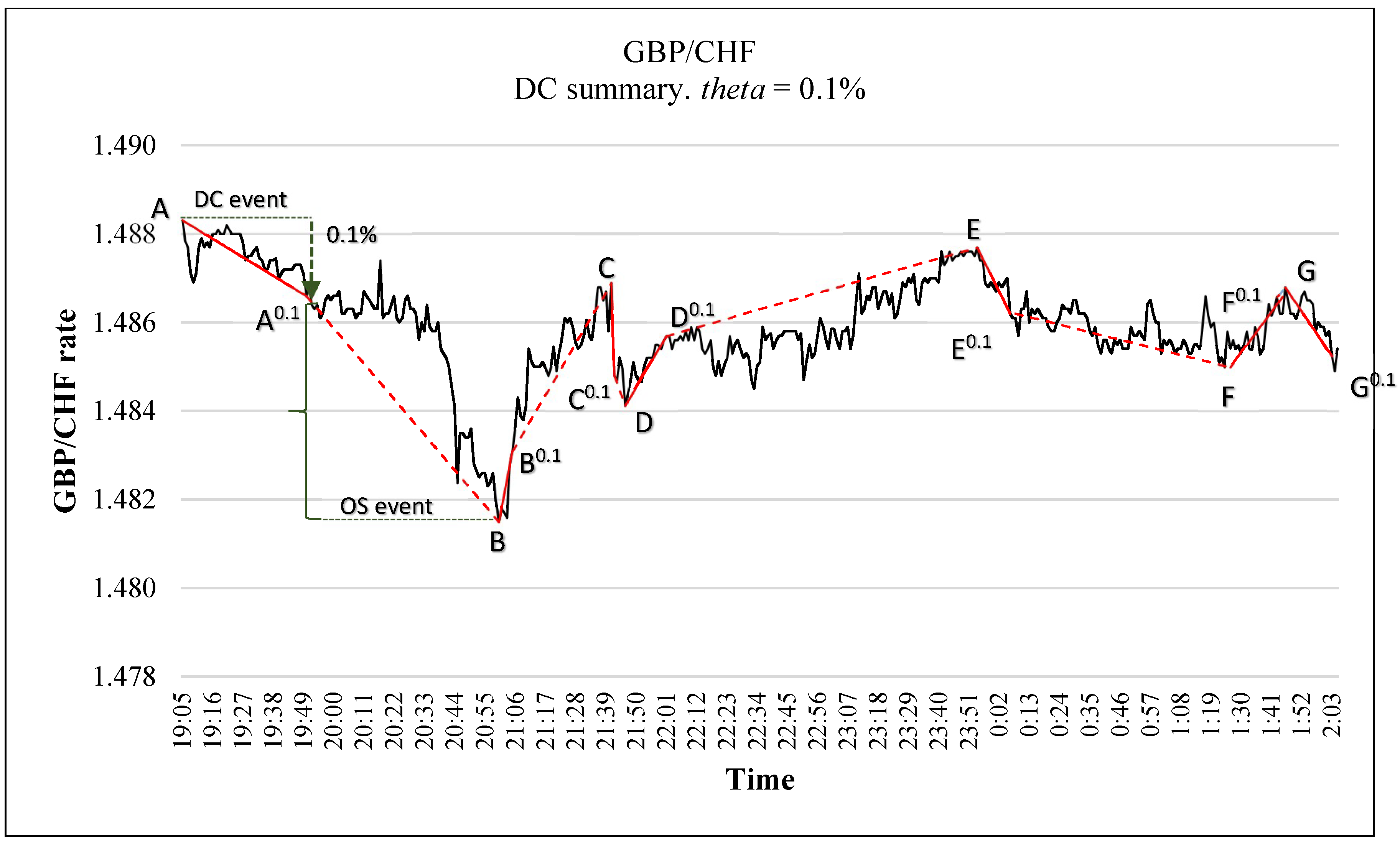
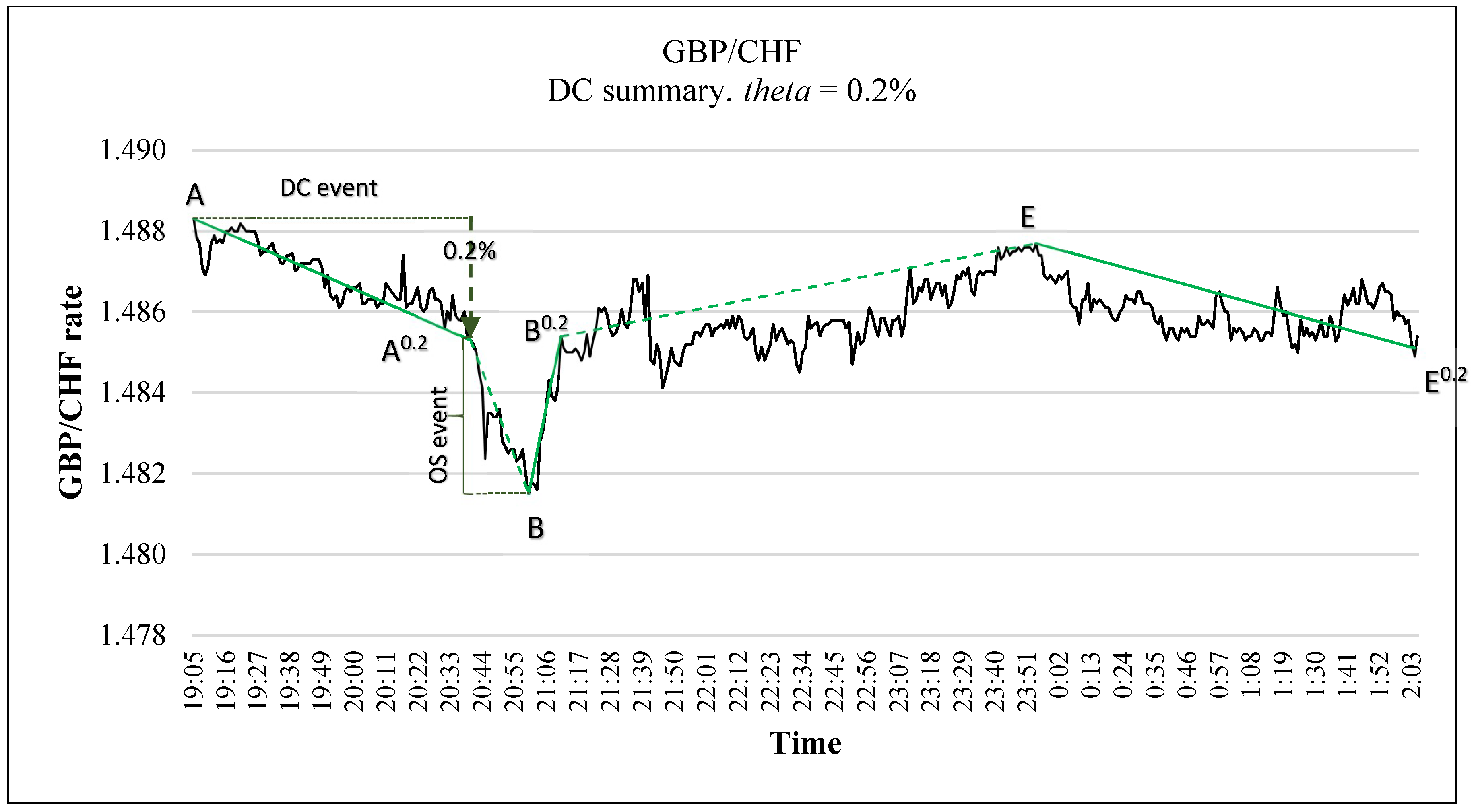
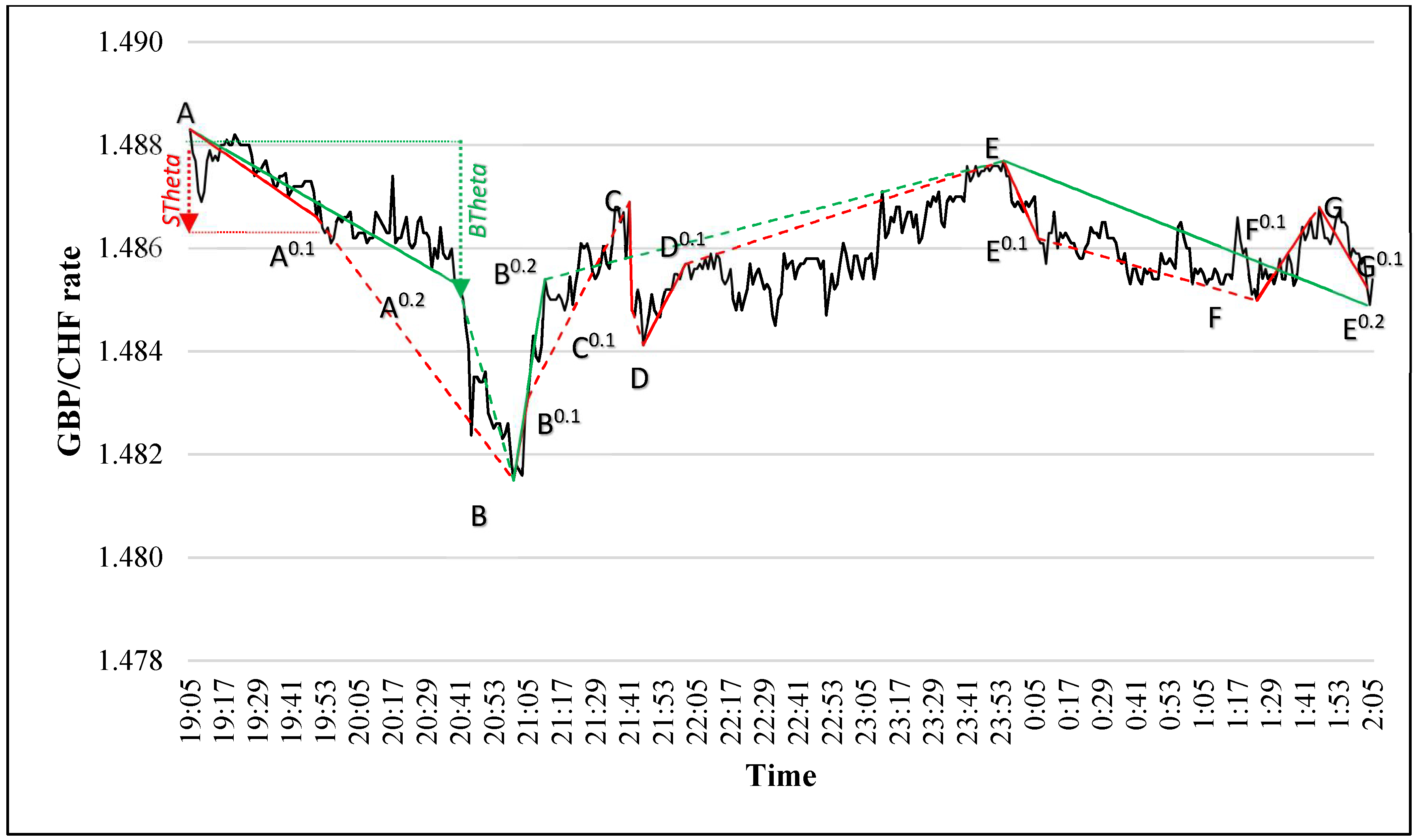
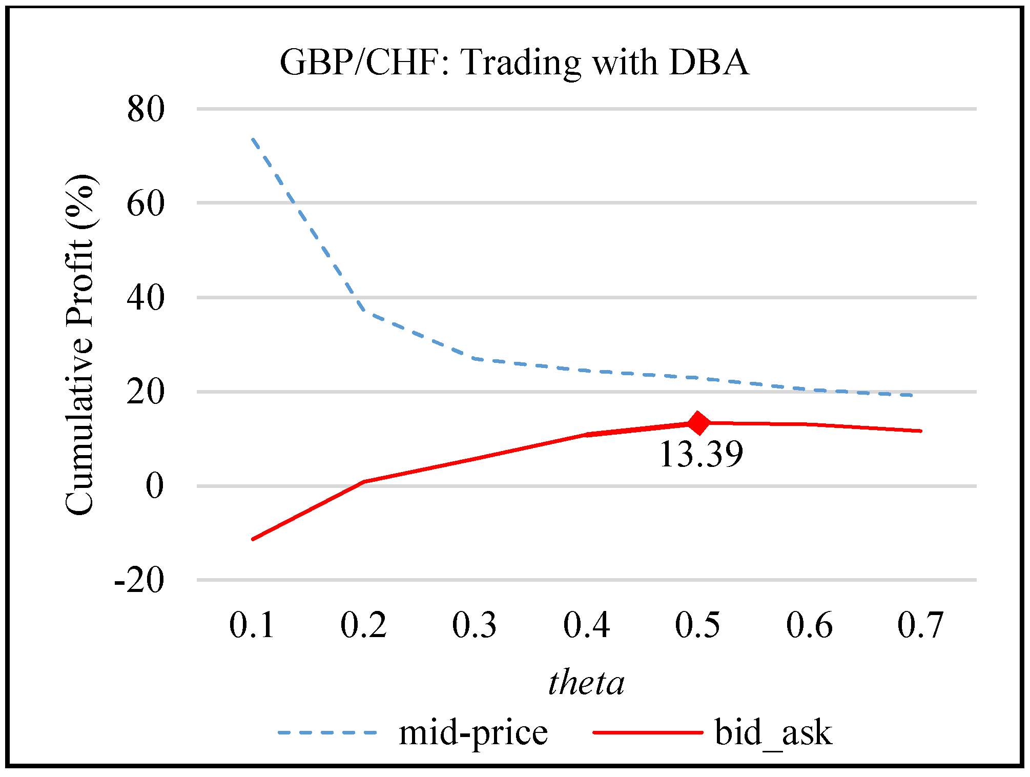
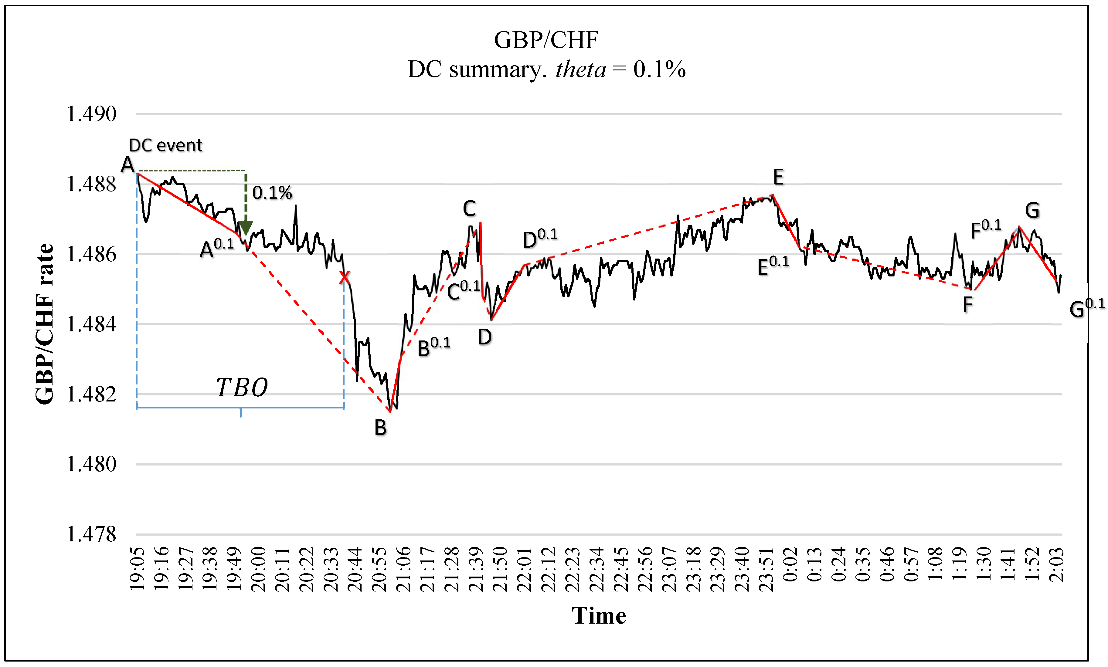
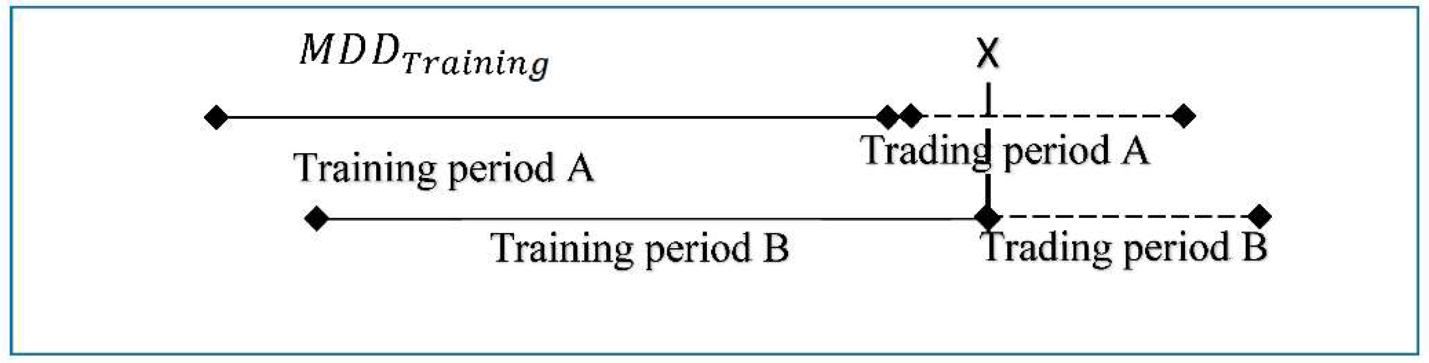
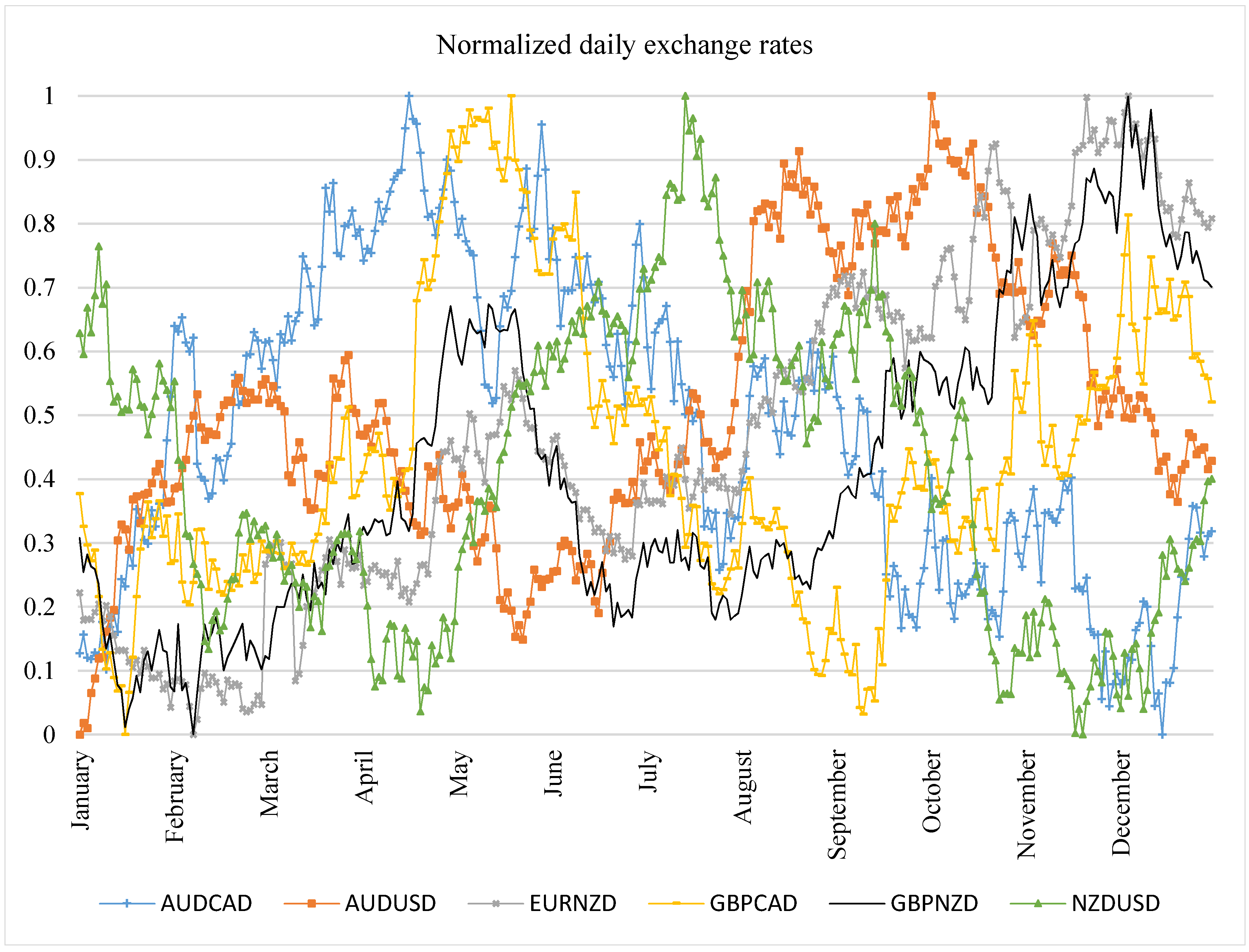
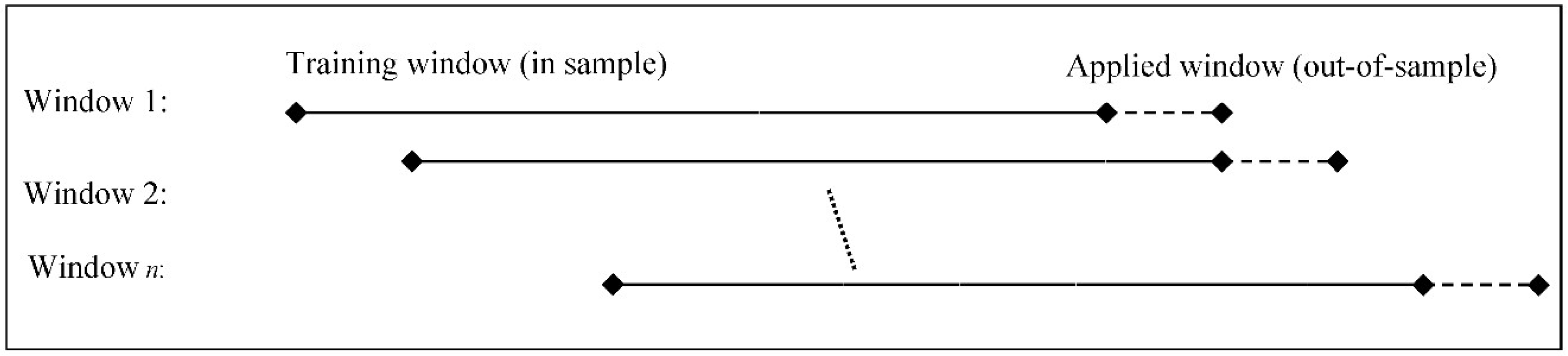
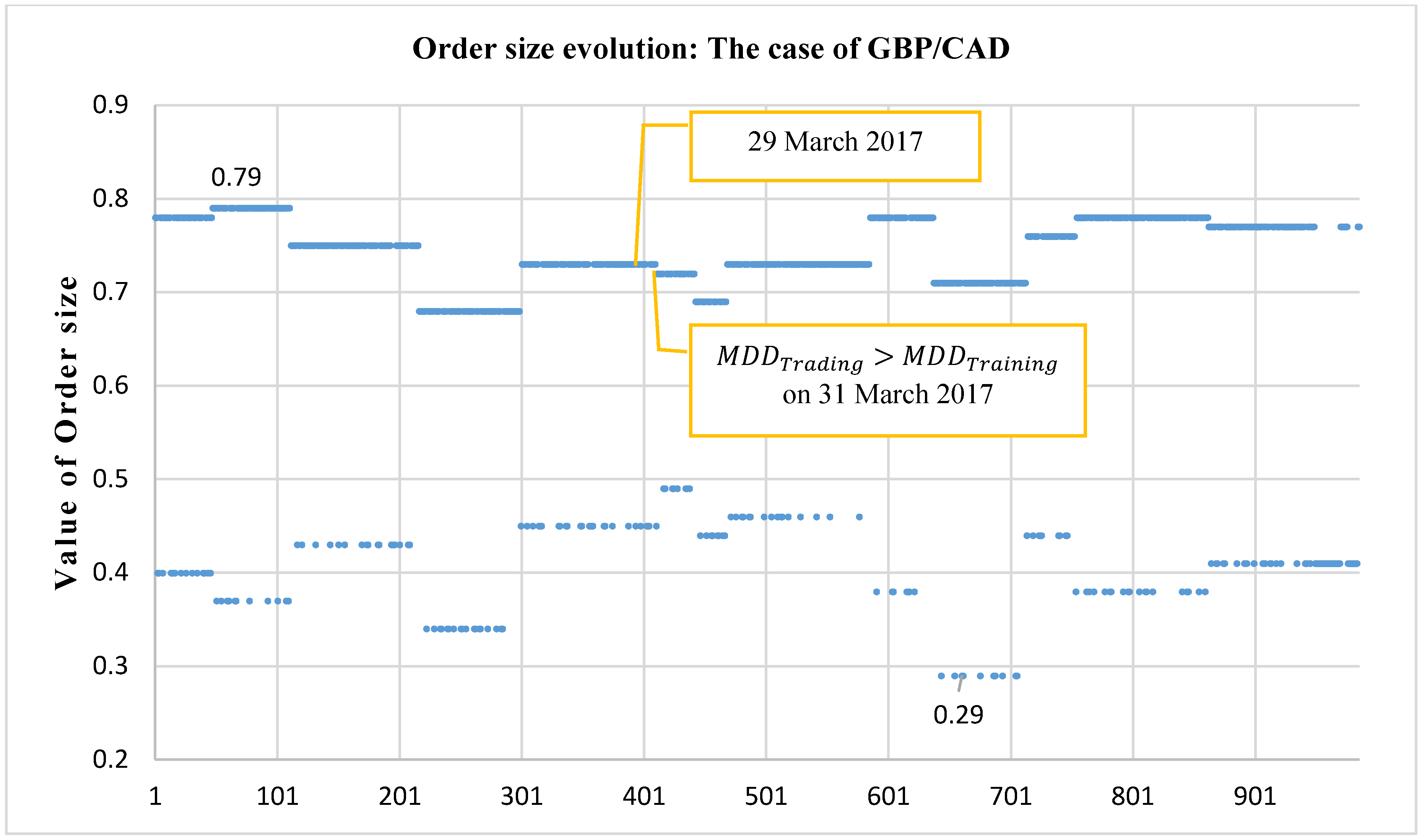
Table 1.
The progress of the value of during the period from 20:55:00 and 21:05:00. According to Figure 1 this period refers to a downtrend. In such a case, refer to the lowest price observed so far during this downtrend.
Table 1.
The progress of the value of during the period from 20:55:00 and 21:05:00. According to Figure 1 this period refers to a downtrend. In such a case, refer to the lowest price observed so far during this downtrend.
| Time | Mid-Price | Point | |
|---|---|---|---|
| 20:55:00 | 1.48260 | 1.48260 | |
| 20:56:00 | 1.48230 | 1.48230 | |
| 20:57:00 | 1.48240 | 1.48230 | |
| 20:58:00 | 1.48260 | 1.48230 | |
| 20:59:00 | 1.48200 | 1.48200 | |
| 21:00:00 | 1.48150 | 1.48150 | B (Extreme point) |
| 21:01:00 | 1.48180 | 1.48150 | |
| 21:02:00 | 1.48170 | 1.48150 | |
| 21:03:00 | 1.48159 | 1.48150 | |
| 21:04:00 | 1.48280 | 1.48150 | |
| 21:05:00 | 1.48310 | 1.48150 | B0.1 (DCC point) |
Table 2.
An example of a DC summary of GBP/CHF mid-prices sampled minute-by-minute from 21:41:00 to 22:01:00on 1 January 2013 (UK time). Excessive and unnecessary observation were omitted. 0.10%. We also compute the values of and .
Table 2.
An example of a DC summary of GBP/CHF mid-prices sampled minute-by-minute from 21:41:00 to 22:01:00on 1 January 2013 (UK time). Excessive and unnecessary observation were omitted. 0.10%. We also compute the values of and .
| Time | Mid-Price | DC Event | Point | ||
|---|---|---|---|---|---|
| 21:41:00 | 1.48690 | start DC event (DOWNTREND) | C | ||
| 21:42:00 | 1.48480 | start OS event (DOWNTREND) | 1.48541310 | C0.1 | −0.41274713 |
| 21:43:00 | 1.48470 | −0.48006847 | |||
| 21:44:00 | 1.48520 | −0.14346177 | |||
| 21:45:00 | 1.48495 | −0.31176512 | |||
| 21:46:00 | 1.48412 | start DC event (UPTREND) | D | −0.87053224 | |
| ……………………… | |||||
| 22:01:00 | 1.48570 | start OS event (UPTREND) | 1.48560412 | D0.1 | 0.0645394 |
Table 3.
An example of a DC summary of GBP/CHF mid-prices sampled minute-by-minute on 1 January 2013 from 21:41:00 to 22:01:00 (UK time). Excessive and unnecessary observation were omitted. 0.10%. We also compute the values of and .
Table 3.
An example of a DC summary of GBP/CHF mid-prices sampled minute-by-minute on 1 January 2013 from 21:41:00 to 22:01:00 (UK time). Excessive and unnecessary observation were omitted. 0.10%. We also compute the values of and .
| Time | Mid-Price | DC Event | Point | ||
|---|---|---|---|---|---|
| 21:41:00 | 1.48690 | start DC event (DOWNTREND) | C | 2.64231213 | |
| 21:42:00 | 1.48480 | start OS event (DOWNTREND) | 1.48541310 | C0.1 | −0.41274713 |
| 21:43:00 | 1.48470 | −0.48006847 | |||
| 21:44:00 | 1.48520 | −0.14346177 |
Table 4.
An illustration of a confusion matrix.
| Actual | |||
|---|---|---|---|
| Predicted | |||
Table 5.
The starting and end dates of each (in-sample) training period and (out-of-sample) trading period for each composed window.
Table 5.
The starting and end dates of each (in-sample) training period and (out-of-sample) trading period for each composed window.
| Rolling Window | Training Period (12 Months) | Trading Period (1 Month) | ||
|---|---|---|---|---|
| From | To | From | To | |
| 1 | 1 January 2016 | 31 December 2016 | 1 January 2017 | 31 January 2017 |
| 2 | 1 February 2016 | 31 January 2017 | 1 February 2017 | 28 February 2017 |
| 3 | 1 March 2016 | 28 February 2017 | 1 March 2017 | 31 March 2017 |
| 4 | 1 April 2016 | 31 March 2017 | 1 April 2017 | 30 April 2017 |
| 5 | 1 May 2016 | 30 April 2017 | 1 May 2017 | 31 May 2017 |
| 6 | 1 June 2016 | 31 May 2017 | 1 June 2017 | 30 June 2017 |
| 7 | 1 July 2016 | 30 June 2017 | 1 July 2017 | 31 July 2017 |
| 8 | 1 August 2016 | 31 July 2017 | 1 August 2017 | 31 August 2017 |
| 9 | 1 September 2016 | 31 August 2017 | 1 September 2017 | 30 September 2017 |
| 10 | 1 October 2016 | 30 September 2017 | 1 October 2017 | 31 October 2017 |
| 11 | 1 November 2016 | 31 October 2017 | 1 November 2017 | 30 November 2017 |
| 12 | 1 December 2016 | 30 November 2017 | 1 December 2017 | 31 December 2017 |
Table 6.
The mean and standard deviation of the bid-ask spread of the selected currency pairs during the trading period (1 January 2017 to 31 December 2017).
Table 6.
The mean and standard deviation of the bid-ask spread of the selected currency pairs during the trading period (1 January 2017 to 31 December 2017).
| Mean | Standard Deviation | Quantile 25 | Quantile 75 | |
|---|---|---|---|---|
| AUD/USD | 0.000061 | 0.000051 | 0.000050 | 0.000060 |
| AUD/CAD | 0.000010 | 0.000090 | 0.000120 | 0.000150 |
| GBP/CAD | 0.000266 | 0.000237 | 0.000190 | 0.000240 |
| GBP/NZD | 0.000508 | 0.000325 | 0.000390 | 0.000480 |
| NZD/USD | 0.000093 | 0.000071 | 0.000010 | 0.000090 |
| EUR/NZD | 0.000347 | 0.000245 | 0.000260 | 0.000320 |
Table 7.
Trading performance of IDBA following the twelve months out-of-sample period (from 1 January 2017 to 31 December 2017) of the six currency pairs.
Table 7.
Trading performance of IDBA following the twelve months out-of-sample period (from 1 January 2017 to 31 December 2017) of the six currency pairs.
| Currency Pair | RR | Profit Factor | Total Number of Trades | Max Drawdown (%) | Win Ratio | Sharpe Ratio |
|---|---|---|---|---|---|---|
| AUD/USD | 23.5 | 1.86 | 1143 | 1.5 | 0.77 | 2.89 |
| AUD/CAD | 26.2 | 1.92 | 1182 | 1.7 | 0.76 | 4.55 |
| GBP/CAD | 4.3 | 1.09 | 986 | 2.6 | 0.64 | 0.83 |
| GBP/NZD | 29.8 | 2.35 | 1892 | 1.7 | 0.78 | 4.62 |
| NZD/USD | 18.8 | 1.42 | 1068 | 3.4 | 0.75 | 1.59 |
| EUR/NZD | 16.1 | 1.87 | 1079 | 2.2 | 0.73 | 1.29 |
Table 8.
Summary of the monthly RR (%) obtained by trading with IDBA to each of the six considered currency pairs. The trading period is from 1 January 2017 to 31 December 2017.
Table 8.
Summary of the monthly RR (%) obtained by trading with IDBA to each of the six considered currency pairs. The trading period is from 1 January 2017 to 31 December 2017.
| Trading Period | AUD/USD | AUD/CAD | GBP/CAD | GBP/NZD | NZD/USD | EUR/NZD |
|---|---|---|---|---|---|---|
| January | 1.4 | 2.0 | 0.7 | 2.0 | 1.9 | 1.2 |
| February | 2.5 | 2.4 | 0.6 | 2.1 | 2.2 | 1.5 |
| March | 0.5 | 2.7 | −0.3 | 2.3 | 1.1 | 2.2 |
| April | 2.4 | 2.5 | −0.2 | 2.4 | 0.1 | 3.2 |
| May | 2.1 | 1.9 | 0.9 | 1.7 | 1.9 | 1.5 |
| June | 1.9 | 2.3 | 0.5 | 2.5 | 2.2 | 2.4 |
| July | 3.0 | 2.4 | 0.6 | 3.6 | 2.5 | 0.4 |
| August | 1.1 | 3.0 | −0.1 | 2.2 | 1.9 | 1.1 |
| September | 2.7 | 2.3 | −0.3 | 2.5 | 1.6 | 1.2 |
| October | 1.8 | 1.1 | 0.7 | 3.4 | 0.8 | 2.0 |
| November | 1.8 | 1.9 | 0.5 | 2.9 | 1.9 | 0.6 |
| December | 2.3 | 1.7 | 0.7 | 2.2 | 2.5 | 0.8 |
| Sum | 23.5 | 26.2 | 4.3 | 29.8 | 18.8 | 16.1 |
Table 9.
Number of times that has exceeded for each of the six considered currency pairs (based on the risk management module described in Section 5.3).
Table 9.
Number of times that has exceeded for each of the six considered currency pairs (based on the risk management module described in Section 5.3).
| AUD/USD | AUD/CAD | GBP/CAD | GBP/NZD | NZD/USD | EUR/NZD |
|---|---|---|---|---|---|
| 6 | 5 | 7 | 6 | 5 | 5 |
Table 10.
Summary of RR and MDD of IDBA and DBA.
| Currency Pairs | RR | MDD | ||
|---|---|---|---|---|
| IDBA | DBA | IDBA | DBA | |
| AUD/USD | 23.5 | 11.2 | 1.5 | 6.7 |
| AUD/CAD | 26.2 | 10.7 | 1.7 | 4.9 |
| GBP/CAD | 4.3 | 3.4 | 2.6 | 5.8 |
| GBP/NZD | 29.8 | 15.5 | 1.7 | 6.5 |
| NZD/USD | 18.8 | −0.7 | 3.4 | 6.2 |
| EUR/NZD | 16.1 | 6.9 | 2.2 | 7.5 |
Table 11.
The p-value of the conducted Wilcoxon tests of comparing the RR and MDD of IDBA and DBA.
| RR | MDD | |
|---|---|---|
| p-value | 0.026 | 0.005 |
Table 12.
Summary of RR and MDD of IDBA and TSFDC.
| Currency Pairs | RR | MDD | ||
|---|---|---|---|---|
| IDBA | TSFDC | IDBA | TSFDC | |
| AUD/USD | 23.5 | 24.2 | 1.5 | 7.8 |
| AUD/CAD | 26.2 | 24.1 | 1.7 | 8.6 |
| GBP/CAD | 4.3 | 5.6 | 2.6 | 12.2 |
| GBP/NZD | 29.8 | 30.5 | 1.7 | 4.6 |
| NZD/USD | 18.8 | 19.7 | 3.4 | 7.4 |
| EUR/NZD | 16.1 | 17.2 | 2.2 | 10.5 |
Table 13.
The p-value of the conducted Wilcoxon tests of comparing the RR and MDD of IDBA and TSFDC.
Table 13.
The p-value of the conducted Wilcoxon tests of comparing the RR and MDD of IDBA and TSFDC.
| RR | MDD | |
|---|---|---|
| p-value | 0.937 | 0.002 |
© 2018 by the authors. Licensee MDPI, Basel, Switzerland. This article is an open access article distributed under the terms and conditions of the Creative Commons Attribution (CC BY) license (http://creativecommons.org/licenses/by/4.0/).
Share and Cite
MDPI and ACS Style
Bakhach, A.; Chinthalapati, V.L.R.; Tsang, E.P.K.; El Sayed, A.R. Intelligent Dynamic Backlash Agent: A Trading Strategy Based on the Directional Change Framework. Algorithms 2018, 11, 171. https://doi.org/10.3390/a11110171
AMA Style
Bakhach A, Chinthalapati VLR, Tsang EPK, El Sayed AR. Intelligent Dynamic Backlash Agent: A Trading Strategy Based on the Directional Change Framework. Algorithms. 2018; 11(11):171. https://doi.org/10.3390/a11110171
Chicago/Turabian StyleBakhach, Amer, Venkata L. Raju Chinthalapati, Edward P. K. Tsang, and Abdul Rahman El Sayed. 2018. "Intelligent Dynamic Backlash Agent: A Trading Strategy Based on the Directional Change Framework" Algorithms 11, no. 11: 171. https://doi.org/10.3390/a11110171
Note that from the first issue of 2016, this journal uses article numbers instead of page numbers. See further details here.