muMAB: A Multi-Armed Bandit Model for Wireless Network Selection

Abstract

Multi-armed bandit (MAB) models are a viable approach to describe the problem of best wireless network selection by a multi-Radio Access Technology (multi-RAT) device, with the goal of maximizing the quality perceived by the final user. The classical MAB model does not allow, however, to properly describe the problem of wireless network selection by a multi-RAT device, in which a device typically performs a set of measurements in order to collect information on available networks, before a selection takes place. The MAB model foresees in fact only one possible action for the player, which is the selection of one among different arms at each time step; existing arm selection algorithms thus mainly differ in the rule according to which a specific arm is selected. This work proposes a new MAB model, named measure-use-MAB (muMAB), aiming at providing a higher flexibility, and thus a better accuracy in describing the network selection problem. The muMAB model extends the classical MAB model in a twofold manner; first, it foresees two different actions: to measure and to use; second, it allows actions to span over multiple time steps. Two new algorithms designed to take advantage of the higher flexibility provided by the muMAB model are also introduced. The first one, referred to as measure-use-UCB1 (muUCB1) is derived from the well known UCB1 algorithm, while the second one, referred to as Measure with Logarithmic Interval (MLI), is appositely designed for the new model so to take advantage of the new measure action, while aggressively using the best arm. The new algorithms are compared against existing ones from the literature in the context of the muMAB model, by means of computer simulations using both synthetic and captured data. Results show that the performance of the algorithms heavily depends on the Probability Density Function (PDF) of the reward received on each arm, with different algorithms leading to the best performance depending on the PDF. Results highlight, however, that as the ratio between the time required for using an arm and the time required to measure increases, the proposed algorithms guarantee the best performance, with muUCB1 emerging as the best candidate when the arms are characterized by similar mean rewards, and MLI prevailing when an arm is significantly more rewarding than others. This calls thus for the introduction of an adaptive approach capable of adjusting the behavior of the algorithm or of switching algorithm altogether, depending on the acquired knowledge on the PDF of the reward on each arm.

1. Introduction

A common experience in everyday’s life is to be connected wirelessly to the Internet: almost everyone uses a device such as a smartphone, a tablet or a laptop, and the Internet connection is now considered as essential, in order to be connected to the rest of the world.

With the many indisputable and undisputed advantages that this situation implies, there are also some new challenges that must be faced. One of them, in the context of cognitive networking and in the scenario where different wireless networks of different technologies (Wi-Fi, UMTS, LTE, …) are present, is the choice of which network to use. Skipping trivial answers and facing the problem from the final user point of view, the question should be expressed like “Which wireless network among the available ones is the one that can offer the best performance in terms of quality perceived by the final user?”

This question is becoming more and more pressing as a result of several concurring phenomena: (1) the increase in computing and processing capabilities of mobile devices, allowing to move decisions from the network to the device; (2) the increasing demands in terms of Quality of Service (QoS) and Quality of Experience (QoE) as perceived by the user; (3) the ever increasing availability of multiple network connections characterized by different characteristics and performance. Efficient network selection will be definitely central in the design and deployment of 5G systems, where the availability of multiple networks and the use of multi-Radio Access Technology (multi-RAT) are expected to be standard operation conditions [1], and multi-tier networks operated in the same geographic area by multiple operators will be a common occurrence [2]. 5G systems will thus require the capability to tackle the network selection problem in both homogeneous scenarios, where all the candidate networks adopt the same technology, and heterogeneous scenarios, where networks using different technologies are available. In the first category fall both the selection of the best cell within a cellular network, and the selection of the best cellular network among different ones, while the second includes, for example, scenarios where both cellular networks and Local Area Networks (LANs) are available. The proposed approaches include game theory [3,4], and the Multi-Armed Bandit model; optimization was also proposed in scenarios where the decision could be taken in a centralized fashion [5], which is, however, less relevant for the user-centric scenario considered in this work.

A proper solution to the user-centric network selection problem requires two main steps: (a) define the QoS/QoE parameters that determine the quality of a network as perceived by the user, and the corresponding utility function; and (b) define the network selection algorithm/strategy that operates by maximizing the selected utility function.

An extensive literature exists on the definition and use of QoS parameters for wireless networks; physical layer parameters such as Received Signal Strength Indicator (RSSI), Signal-to-Noise Ratio (SNR), Signal-to-Interference Ratio (SIR) and Bit Error Rate (BER) have been widely adopted to enforce QoS policies, often in conjunction with Medium Access Control (MAC) layer parameters such as frame error rate, throughput, delay, jitter and collision rate, and network layer parameters such as packet error rate, end-to-end delay and throughput; an extensive survey on QoS parameters and corresponding utility functions can be found in [4]. More recently, research focused on translating QoS parameters into Key Performance Indicators (KPIs) capable of reliably expressing the QoE perceived by the user for each specific class of traffic/applications [6,7]. The choice of the parameters taken into account in the definition of the utility metric and, in particular, the resulting rate of variation over time of the metric, will have a strong impact on the performance of network selection strategy, and should be considered in the decision on the network selection approach to be adopted.

Moving to algorithms and mathematical approaches proposed for network selection, game theory was widely proposed as a solution in cases where no central processing point is available, and cooperation between users may or may not be available. In homogeneous scenarios, game theory was proposed in [8], among others, as a way to select the best cell in two-tier network, and in a broader scheme, in combination with a machine learning algorithm, to solve the problem of best provider selection and power allocation within the selected network [9]. In heterogeneous scenarios, game theory was adopted in [10] to jointly tackle the network selection and resource allocation problems in a multi-operator heterogeneous network in which users take simultaneous decisions; the paper also provided an extensive analysis of the use of game theory for network selection, including the issue of the definition of utility metrics to be adopted in the problem. In [11], the problem was extended by considering a game in which users take their network selection decisions sequentially, taking into account decisions of other users.

A reasonable assumption in the network selection problem is, however, that no a priori information about the networks is available, except for their presence, requiring thus the acquisition of measurements of relevant networks parameters in order to enable an informed decision on the network to be selected. The Multi-Armed Bandit (MAB) framework, in which a player chooses among different arms with the goal of maximizing a reward, can be used to model the above problem [12,13,14] . In fact, by using Peter Whittle’s words [12], MAB problems embody in essential form a conflict evident in all human actions. This is the conflict between taking those actions that yield immediate reward and those (such as acquiring information or skill, or preparing the ground) whose benefit will come only later. In the considered scenario, the action with future benefit is to measure network parameters, while connecting to a network and exploiting it for transmitting and receiving is the action with immediate reward. The idea of adopting an online learning algorithm is indeed in line with recent proposals for best network selection in 5G, foreseeing complex information acquisition phases involving both devices and network infrastructure for an effective network selection [15]. Current MAB models focus, however, mainly on actions that bring an immediate reward: existing algorithms built on the basis of such models mainly address thus how to decide which arm, i.e., which wireless network in the considered case, to select at each time step [16,17,18]. This is also the case for online learning algorithms based on the MAB model proposed to address the network selection problem, as for example the one in [19], where a continuous time MAB problem is solved in order to select the network providing the best QoE to the user.

This work proposes a a new MAB model that takes into account the need for a measurement phase before the network selection decision can take place, introducing thus a trade-off between the time $T_M$ dedicated to measuring the performance of each network, and the time $T_U$ spent using the selected network before updating again the information on available networks. On the one hand, $T_M$ should be long enough to guarantee an effective decision; on the other, it should be significantly shorter than $T_U$, in order to ensure that the overhead related to measuring, expressed by the ratio $T_M/\left(T_M+T_U\right)$, is kept at a reasonable level.

The new MAB model, referred to as measure-use-MAB (muMAB), allows the player to select between two distinct strategic actions: measure and use. Since existing arm selection algorithms cannot take advantage of the new possibilities opened by the presence of two possible actions, two new algorithms specifically designed on the basis of the muMAB model are also introduced, referred to as measure-use-UCB1 (muUCB1) and Measure with Logarithmic Interval (MLI).

The impact of the muMAB model is analysed by evaluating the performance obtained in its context by several algorithms widely used in literature, and by the two newly proposed algorithms.

The paper is organized as follows: Section 2 introduces the muMAB model and the muUCB1 and MLI algorithms. Section 3 introduces the experimental settings, while the results are presented and discussed in Section 4. Finally, Section 5 concludes the work.

2. Measure and Use Differentiation in Multi-Armed Bandit

2.1. The muMAB Model

The classical MAB model foresees different arms, each of them characterised by a reward, modeled by a random variable with a fixed (unknown) mean value. At every step, an arm is selected and its current reward value is obtained as feedback.

Many algorithms, also called strategies or policies, were proposed in literature in order to identify and choose as soon as possible the arm with the highest mean reward without any a priori knowledge, except for the number of arms [16,17]. Their performance is usually expressed in terms of regret, which is the difference between the cumulative reward obtained by always choosing the arm with the highest mean and the cumulative reward actually obtained with the chosen arms. Regret was first proposed as evaluation parameter for algorithms performance in [20]; it was later shown that, in terms of regret, the best performance an algorithm can achieve is a regret that grows logarithmically over time [16].

In the classical MAB model, there is only one possible action: to select an arm and collect the corresponding reward. In real world scenarios, however, such as the best wireless network selection considered in this work, the selection phase is preceded by a measurement phase, in order to support an informed decision. Furthermore, the selection is usually kept unchanged for a significant time, typically much longer than the time dedicated to measuring the performance of the candidate networks. This is due to the overhead introduced by a network switching procedure, as well as to the discomfort caused to the user due to service interruption during network switch; indeed, a significant effort was devoted to designing algorithms that prevent frequent network switching procedures [21]. The muMAB model is designed so to grasp the cycle between measuring and using, and thus model real scenarios with higher accuracy than the classical MAB model. The muMAB model can be described as follows:

• time is divided into steps with a duration of T, and the time horizon is defined as $T_{TH}=n_{TH}T$;
• there are 1 player and $\mathcal{K}$ arms;
• a reward is associated with the generic k-th arm, $k=\{1,\cdots ,\mathcal{K}\}$; $\forall k\in \mathcal{K}$, the reward $\left\{W_k\left(n\right):n\in N\right\}$ is a stationary ergodic random process associated with arm k, with statistics not known a priori; given a time step n, $W_k\left(n\right)$ is thus a random variable taking values in the real non-negative numbers set ${\Re }^{+}$, with unknown Probability Density Function (PDF); the mean value of $W_k\left(n\right)$ is defined as ${\mu }_k=E\left[W_k\left(n\right)\right]$;
• there are two distinct actions: to measure (“m”) and to use (“u”). At the beginning of time step n, the player can choose to apply action a to arm k; the choice $c_n$ is represented by a pair:

  $$c_n=\left(a_n,k_n\right),a_n\in \left\{m,u\right\},k_n\in \mathcal{K},$$

  (1)

  which means that, at time step n, the arm $k_n$ has been chosen with an action $a_n$; every choice $c_n$ obtains feedback $f\left(c_n\right)$;
• feedback $f\left(c_n\right)$ is a pair, composed by:
  • a realization of $W_k\left(n\right)$ at time step n, $w_k\left(n\right)$, that is the current reward value associated with arm k;
  • a gain $g\left(c_n\right)$;
  therefore:

  $$f\left(c_n\right)=\left(w_k\left(n\right),g\left(c_n\right)\right);$$

  (2)
• measure and use actions have duration $T_M$ and $T_U$, respectively, defined as $T_M=n_{M}T$, $T_U=n_{U}T$, where $n_M,n_U\in N$. As a result, if at time step n the player chooses action measure (use, respectively), i.e., $a_n=m\left(a_n=u\right)$, the next $n_M$ ($n_U$) steps are “occupied” and the next choice can be taken at time step $n^{\prime }=n+n_M$ ($n^{\prime }=n+n_U$). Gain $g\left(c_n\right)$ is a function of both the selected action and $W_k\left(n\right)$; it is always equal to zero when measure action is selected, while it is the sum of the values of the realizations of $W_k\left(n\right)$ from time steps n to $n^{\prime }=n+n_U$ when arm k is used at time step n:

  $$g\left(c_n\right)=\left\{\begin{array}{cc}0,\hfill & \mathrm{if}{a}_n=m,\\ \sum _{i=n}^{n+n_U}{w}_k\left(i\right),\hfill & \mathrm{if}{a}_n=u;\end{array}\right.$$

  (3)
• the performance of an algorithm is measured by the regret of not always using the arm with the highest reward mean value $k^{\ast }$:

  $$k^{\ast }=\underset{k\in \mathcal{K}}{arg\; max}{\mu }_k;$$

  (4)

  regret at time step n is defined as:

  $$R\left(n\right)=G_{MAX}\left(n\right)-E\left[G\left(n\right)\right],$$

  (5)

  where:

  $$G\left(n\right)=\sum _{i=1}^{n}g\left(c_i\right),$$

  (6)

  with i used as index of time steps where an action can be taken (i.e., excluding the time steps “occupied” by preceding decisions: measure occupies the following $n_M$ time steps while use occupies the following $n_U$ time steps), and $G_{MAX}\left(n\right)$ is the maximum possible cumulative gain at time step n, obtained by always using the arm $k^{\ast }$ (and never measuring):

  $$G_{MAX}\left(n\right)=E\left[G\left(n\right)\right]:c_i=\left(u,k^{\ast }\right);$$

  (7)
• the goal is to find an algorithm that minimizes regret evolution in time.

In the muMAB model, both actions provide, as part of their feedback, the value of the current reward on the arm measured or used, and allow thus the player to use this information in order to refine the estimation of the mean value of the reward of the selected arm.

The key difference between the two actions is in the time span required to collect this information: since, in fact, usually $T_M<T_U$ in real cases, when use is selected, the player will have to wait a longer time span before deciding to switch to another arm based on the collected reward values. On the other hand, if the player selects the action use on a given arm, the resource is effectively exploited and there is, therefore, an immediate gain. The choice of measuring an arm, instead, permits obtaining a more accurate estimate of the performance achievable with that arm (if it will be used in future steps) in a shorter time; this comes, however, at the price of a null gain for the entire measure period, i.e., for $T_M$.

The muMAB model differs thus from the classical MAB model under the following aspects:

• it introduces two actions, measure and use, in place of the use action considered in the classical model;
• as a result of each action, it provides feedback composed of two parts: the values of the rewards on the selected arm, and a gain depending on the selected action;
• it introduces the concept of locking the player on an arm after it is selected for measuring or using, with different locking periods depending on the selected action (measure vs. use).

These new features make the muMAB better suited to represent real world scenarios, in which a measuring phase precedes the decision on which resource to use.

It is worth noting that different wireless networks might require different measurement and use periods, depending on the characteristics of the specific network. Nevertheless, any network selection algorithm will require the adoption for each of the two parameters of a common value to all networks, since a decision on which network to select will have to be guaranteed within a finite time. In the following, the determination of the values to be adopted for $T_M$ and $T_U$ will be assumed to be the result of a compromise between the optimal values that would be required for each of the candidate networks.

2.2. Algorithms

Two algorithms that are able to exploit the difference between measure and use are proposed in this work: muUCB1 and MLI.

2.2.1. muUCB1

muUCB1 derives from the well known and widely used UCB1 algorithm [16]; the choice of proposing an algorithm derived by UCB1 is justified by the fact that UCB1 is often used as a benchmark in the evaluation of MAB selection algorithms because it reaches the best achievable performance, i.e., a regret growing logarithmically over time, but at the same time presents a low complexity.

In the following, the UCB1 algorithm is briefly described, focusing on aspects that are relevant to the proposed muUCB1 algorithm; a more detailed description of UCB1 can be found in [16].

UCB1 operates by associating an index to each arm, and selecting the arm characterized by the highest index. The value of the index is determined by the sum of two elements:

• the reward mean value estimate of the arm;
• a bias, that eventually allows the index of an arm with a low reward mean value to increase enough for the arm to be selected.

The index of arm k is therefore:

$$I_k={\widehat{\mu }}_k+\sqrt{\frac{2ln\left(N\right)}{N_k}},$$

(8)

where $N_k$ is the number of times arm k has been selected so far and N is the overall number of selections done so far (equivalent to the number of steps n, if considering the classical MAB model).

The arm with the highest index at time step n is selected and the index of every arm is updated. Normally, the arm with the highest reward mean estimate also has the highest index, and is therefore selected. This corresponds to an exploitation in MAB terms, that is to say that the available information is exploited for the arm choice. Eventually, however, the bias significantly affects the index value, leading to the selection of an arm that does not present the highest reward mean estimate. This corresponds to an exploration in MAB terms; in other terms, previously acquired information is not exploited for the choice, but another arm is “explored”, and its estimate is updated.

muUCB1 inherits from UCB1 the rule for the arm selection: when the arm $k_{IND}$ with the highest index corresponds to the one with the highest reward estimate, $k_{EST}$, the selected action is use. When the arm with the highest index is not the one with the highest reward estimate, the selected action is measure. This choice creates an ideal correspondence between measure and exploration on one hand, and use and exploitation on the other.

The pseudo code of the algorithm is reported in Algorithm 1.

2.2.2. MLI

MLI is an algorithm designed from scratch to fully exploit the new muMAB model. It is divided in two phases, identified as Phase 1 and Phase 2. Phase 1 is completely dedicated to collecting measurements, with the goal of building up a “reliable enough” estimate for each arm’s reward mean value. Every arm k is measured $d_1^k$ times according to a round robin scheduling. The duration of Phase 1 is, therefore, equal to:

$$T_{PH1}=\sum _{k=1}^{\mathcal{K}}{d}_1^k{T}_M,$$

(9)

and the estimate of the reward for each arm is set to the average of the $d_1^k{T}_M$ realizations of $W_k\left(n\right)$ obtained for that arm.

Since during Phase 1 only measure actions are performed, the resulting gain is null during $T_{PH1}$. It is, therefore, desirable to limit its duration to the shortest possible period. $d_1^k,k=\left\{1,\cdots ,\mathcal{K}\right\}$ can be set to the same value for all arms, leading to $d_1^k=d_1\forall k$, with $d_1$ to be selected based on the rewards obtained as feedback during the first round of measurements: the idea is that the closer to each other the obtained values are, the higher the $d_1$ value must be, so that the estimates are reliable enough to support effective arm selection during Phase 2. If the first measurements show that arms reward mean values are significantly different among them, a low value for $d_1$ could be selected in order to keep $T_{PH1}$ as short as possible. As an alternative, each arm k can be measured a different number of times, e.g. spending more measuring actions on arms for which the variance of the measurements is higher, while interrupting sooner the measurements for arms showing a low variance in rewards.

Algorithm 1: muUCB1.

Phase 2 of the MLI algorithm is mostly dedicated to use actions, with the exception of sporadic measure actions, as explained in the following. Based on estimates built up during Phase 1, the algorithm starts exploiting the resource by using the arm with the highest estimated reward mean value, obtaining as feedback a gain and a reward realization, which is used to update the arm’s reward estimate. Periodic measure actions are, however, performed in order to update the estimates of the mean values of the rewards for the other arms. The first measure is performed after $d_2$ use actions; the interval between two consecutive measures grows then logarithmically over time. In particular, arms are measured at time steps $n_i$ such that

$$n_i=\lceil n_{i-1}+ln\left(n_{i-1}\right)\rceil ,$$

(10)

with:

$$i\ge 1,n_0=d_2{n}_U>1.$$

(11)

The arm chosen for being measured is the one whose reward estimate is based on the lowest number of values. This can later be changed, by choosing to measure the arm with the “oldest” updated estimate, the one with the second highest estimate (since it can be the most critical value) or a combination of these three solutions. In all the other time steps, the arm with the current highest reward estimate is always used.

The pseudo code of the algorithm is reported in Algorithm 2, assuming for simplicity to adopt the approach $d_1^k=d_1\forall k$.

Algorithm 2: MLI.

2.3. muMAB Complexity and Discussion

The muMAB model, and the corresponding muUCB1 and MLI proposed algorithms, do not significantly increase the overall complexity required to the system (e.g., the end-user device), toward the best arm (e.g., the best network) identification and selection, when compared to typical MAB model and algorithms.

On the one hand, muMAB introduces the measure action, which is used to enhance the reward estimate on an arm not currently selected (e.g., enhance the performance estimate on a candidate access network), without properly selecting that arm (e.g., without setting up a connection switching toward that candidate network, and thus starting a real data exchange), which is instead the use action (It is worth pointing out that, as described in Section 2.2.1, exploitation vs. exploration MAB options both refer to the use action in the proposed muMAB model). In the context of network selection, the measure action may involve several operations, such as simple probe connections, and/or control message exchange with the candidate networks, in order to gather information on the ongoing performance of such networks, and also to estimate parameters that can be useful for the optimization of the next use action. This procedure, generally known as context retrieval, is envisioned in recent standards for network selection, that in fact promote so-called context-aware network selection, thus explicitly requiring measure actions; when considering, for example, recent and future mobile cellular system generations, and expected and desirable interoperability with WLAN technologies, such as WiFi, standards like 3GPP Access Network Discovery and Selection Function (ANDSF), and IEEE 802.21 Media Independent Handover (MIH) are considered as enablers for the above selection mechanisms, and may be thus nicely modeled by muMAB [15]. Algorithms operating within the muMAB model are expected to show a complexity comparable to the one observed in the classical MAB model, since the introduction of the context retrieval does not, in general, foresee operations that are, from the device point of view, more complex or energy-consuming than real data exchange. Regarding performance comparison in terms of regret increase over time, it is reasonable to assume that the particular information gathered during the context retrieval will affect the regret behavior, depending on how such information can be used for a reliable estimate of the reward on each candidate network; however, in the present work, the muMAB algorithms foresee a measure action that provides direct reward measurements, and thus, in this case, an asymptotic logarithmic regret increase can be safely assumed for muUCB1 and MLI, similarly to what happens in the original UCB1 algorithm [16] (The analysis of the effect of gathering different information in the context retrieval, possibly having different reliability and impact on the network reward estimate, is out of the scope of this work and thus left for future research).

On the other hand, muMAB introduces the concept of locking a player on an arm, with a different locking duration depending on the selected action. From a network selection perspective, this assumption makes the model more realistic, if proper settings are adopted, such as (a) a reasonable configuration of duration and periodicity of measure vs. use actions, aiming at minimizing the time spent for context retrieval, since this operation nullifies short-period gains, and (b) a reasonable number of user switching between different networks over time, in order to avoid so-called ping-pong effects, which significantly impact device energy consumption and overall network stability. When compared to the MAB model, the effect of locking is to decrease the rate of actions, thus possibly decreasing the overall complexity; in a fair comparison, however, this effect has to be taken into account for both esisting and newly proposed algorithms, having thus no effect on the comparison of complexities between the different algorithms. When considering the regret increase over time, it is reasonable to assume that the duration of measure vs. use locking periods, and their ratio, will affect the regret behavior in the finite-time regime, that is, in the regret values at each time step [16,22], while the impact can be considered negligible in the asymptotic regime, that is at the time horizon (This work heuristically confirms the above insights, as showed in the simulation results presented and discussed in Section 3. Closed-form expressions for finite-time regret bound analysis are left for future work).

3. Performance Evaluation: Settings

Tests on the impact of the introduction of the proposed model were carried out through simulations. Performance in terms of regret of six different algorithms was compared.

The tested algorithms are the following:

• UCB1 [16];
• muUCB1;
• MLI;
• $\epsilon$-greedy [23];
• $\epsilon$-decreasing [16,22];
• POKER [17].

The last three algorithms listed above were not previously presented, and are briefly introduced in the following; in all of them, the action performed is always use, but they differ in the rules adopted for selecting the arm.

The $\epsilon$-greedy is extremely simple: it selects a random arm with probability $\epsilon$, and the arm that led to the highest cumulative rewards otherwise.

The $\epsilon$-decreasing is a variation of the $\epsilon$-greedy in which the probability $\epsilon$ to select a random arm decreases with the time index n; one has in particular $\epsilon \left(n\right)=min\left\{1,\frac{{\epsilon }_0}{n}\right\}$ in the version analyzed in [16] and implemented in this work.

The Price of Knowledge and Estimated Reward (POKER) algorithm was proposed in [17]; the algorithm combines three ideas in determining the next arm to be selected: (a) assign a value to the exploration of an arm defined in the same units used for rewards; (b) use data collected for other arms to generate a priori knowledge on arms not yet used, assuming correlation between different arms; (c) take into account the time remaining until the time horizon is reached in order to decide whether to exploit or to explore; the algorithm performed quite well when applied to real, captured data. A detailed description of the algorithm and of its performance over captured data can be found in [17].

All the six algorithms listed above where tested against both synthetic and captured data. The simulations were performed considering different $T_U/T_M$ ratios. The case where $T_U=T_M$ was included in the analysis as a baseline setting although, as discussed in Section 1, it can be expected that in real scenarios a measure action will require a shorter time than a use action, i.e., usually $T_M<T_U$. Increasing $T_U/T_M$ ratios can represent scenarios where the network switch process is increasingly costly in terms of overhead or user dissatisfaction, leading to longer use periods before a switching procedure can take place.

Simulation settings common to both synthetic and real data are the following:

• the number of steps required to reach the time horizon was set to $n_{TH}={10}^5$;
• $\mathcal{K}=5$ arms were considered;
• the value of $n_M$ was set to 1; therefore, $T_M=T$; the value of $n_U$ was variable, leading to different $T_U/T_M$ ratios being considered;
• for $\epsilon$-greedy algorithm, $\epsilon$ was set to $0.1$ according to the results presented in [17], indicating this value as the one leading to best performance;
• again, according to [17], in the $\epsilon$-decreasing algorithm, ${\epsilon }_0$ was set to 5;
• for the MLI algorithm, the number of times that every arm is measured in the Phase 1 was set to $d_1=5$; $d_2$, i.e., the number of use actions after which the first measure is performed, was also set to 5;
• all results were averaged over 500 runs;

Information specific to synthetic and real data used in the experiments are presented in Section 3.1 and Section 3.2, respectively. Results of the experiments are presented and analysed in Section 4.

3.1. Synthetic Data

Synthetic data were generated according to three different distributions for the reward PDF, that are the most used ones in MAB literature:

• Bernoulli distribution;
• truncated (to non-negative values) Gaussian distribution;
• exponential distribution.

Two different configurations were considered for the reward mean values (or success probabilities, when considering the Bernoulli distribution) ${\mu }_k,k=1,\cdots ,\mathcal{K}$:

• Hard configuration: ${\mu }_1=0.6$, ${\mu }_2=0.8$, ${\mu }_3=0.1$, ${\mu }_4=0.3$, ${\mu }_5=0.7$;
• Easy configuration: ${\mu }_1=0.2$, ${\mu }_2=0.8$, ${\mu }_3=0.1$, ${\mu }_4=0.3$, ${\mu }_5=0.1$.

The best arm is therefore arm number 2 in both configurations, but, in the Hard one, three different arms have similar mean rewards, making it easier for algorithms to erroneously pick a sub-optimal arm.

3.2. Real Data

As for the captured data, the same datasets used for tests presented in [17] were used, since they were made available by the authors. Data consist in the latencies measured when visiting Internet home pages of 760 universities, with 1361 measured latencies for each home page. Latencies are measured in milliseconds, and are provided in the form of a 1361 by 760 matrix, where each column represents the latency measured in collecting a data sample from one of the webpages.

Table 1. Excerpt from the data used in [17], downloaded from [24]; data express latencies measured in milliseconds.

Acu-Edu	Acadiau-Ca	Adrian-Edu	Agnesscott-Edu	Aims-Edu
396	381	488	506	333
271	261	488	504	276
271	141	325	545	266
268	136	324	1946	331
273	136	321	549	290

presents an excerpt of the data in the form of a 5 by 5 submatrix; the full data set can be downloaded from [24].

These data, even if captured through a single cabled network, can represent the performance that different wireless networks offer; they are therefore particularly interesting for the test of the muMAB model, whose aim is to better fit real world scenarios. Further details about the data and the capture process can be found in [17].

Given the generic i-th latency sample for the j-th website $l\left(i,j\right)$ two different functions were considered in order to obtain the corresponding non-negative reward $r\left(i,j\right)$ required by the muMAB model:

(1)

$r\left(i,j\right)=l_{max}-l\left(i,j\right)$ (linear conversion);

(2)

$r\left(i,j\right)=\frac{log\left(l_{max}\right)-log\left(l\left(i,j\right)\right)}{log\left(l_{max}\right)}$ (logarithmic conversion),

where $l_{max}$ is the maximum latency in the entire data set.

In each run, five random arms among the 760 ones were picked up; then, for each selected arm in each run, the 1361 available values were randomly sorted, and then repeated in order to reach the required $n_{TH}$ time steps.

4. Performance Evaluation: Results

This section presents simulation results, and is organized in five subsections. Section 4.1 presents results obtained when considering synthetic rewards generated using the Hard configuration, while Section 4.2 presents results obtained in the Easy configuration. Next, Section 4.3 presents results obtained using real data and linear conversion, while Section 4.4 analyzes the effect of the logarithmic conversion. Finally, Section 4.5 discusses and compares the results presented in the previous subsections.

A general consideration can be done before analyzing the results: the two proposed algorithms, muUCB1 and MLI, cannot achieve any performance gain with respect to the other algorithms when $T_U=T_M$. In this case, in fact, the measure action lasts as long as the use one, but obtains no gain, making it impossible for the proposed algorithms to obtain a smaller regret than the one achieved by algorithms that always select a use action, and therefore get a gain for exploiting the resource, while also refining the estimation of mean value of reward for the selected arm.

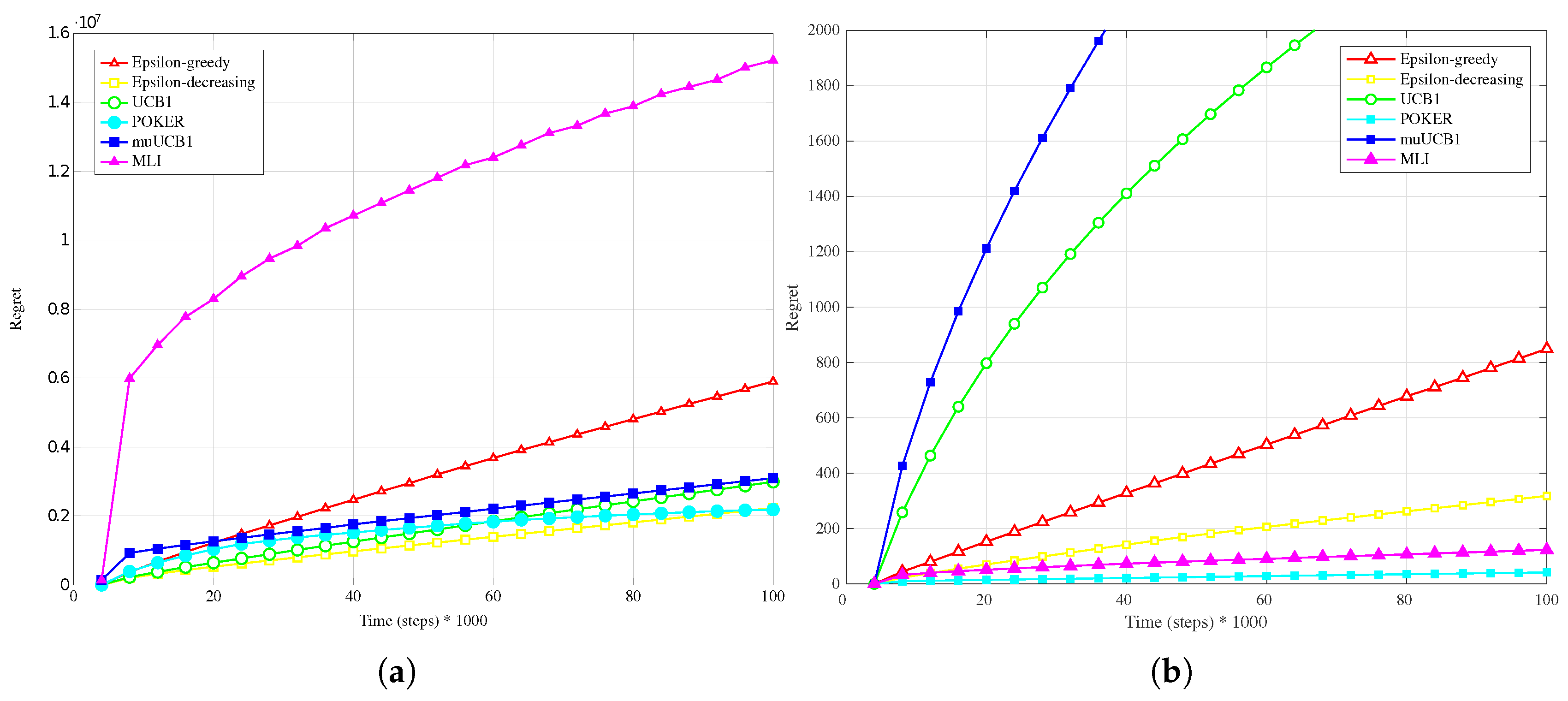
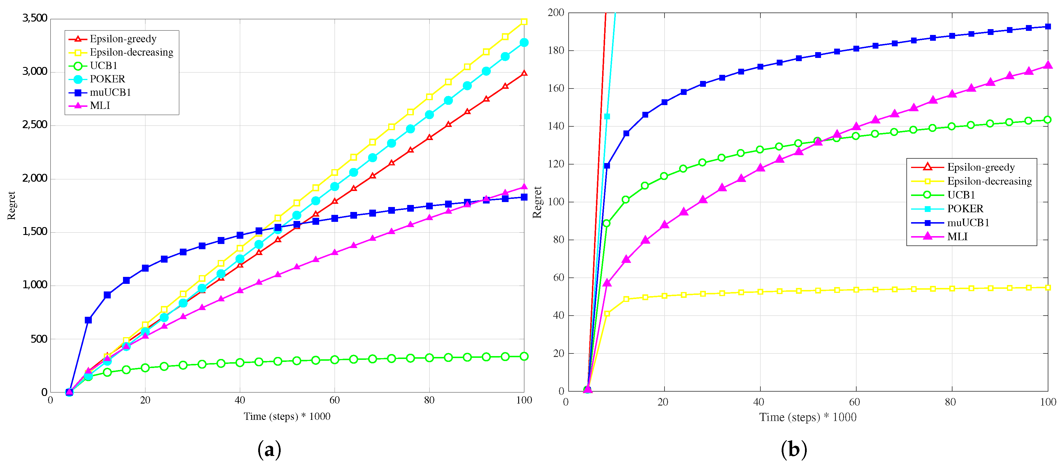
4.1. Synthetic Data-Hard Configuration

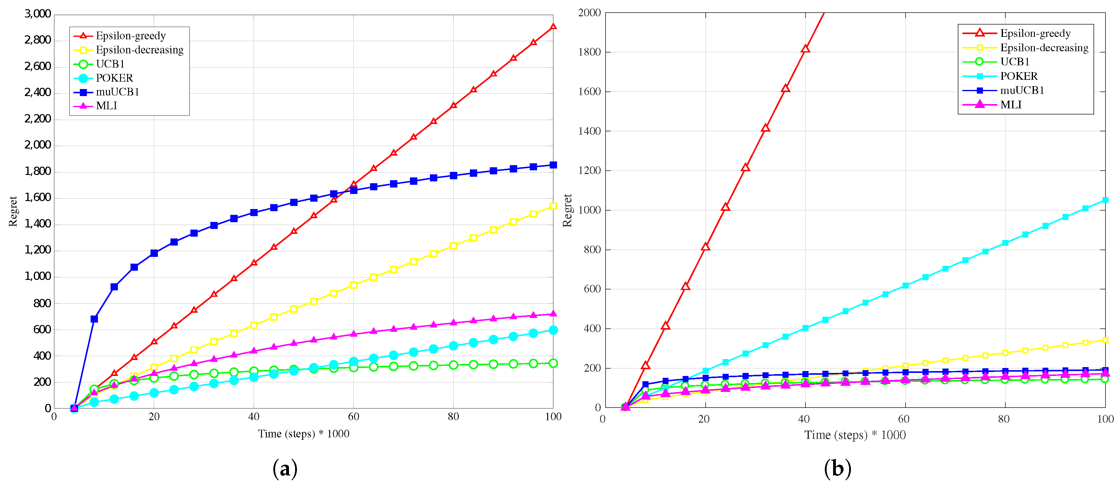
Figure 1a, Figure 2a and Figure 3a present results when a Bernoulli distribution is adopted for the reward PDF in the Hard configuration. In this case, the POKER algorithm is the algorithm that presents best overall behavior and leads to the lowest regret at the time horizon for $T_U/T_M=5$ and $T_U/T_M=10$, while UCB1 provides the best performance at the time horizon when $T_U=T_M$. Moving to the new algorithms, their performance compared to the other ones improves as the $T_U/T_M$ ratio increases; this is true in particular for muUCB1, that moves from an extremely bad performance when $T_U/T_M=1$ to a regret comparable to the POKER algorithm when $T_U/T_M=10$, furthermore showing a trend as a function of time suggesting that muUCB1 might be the best option on a longer time horizon.

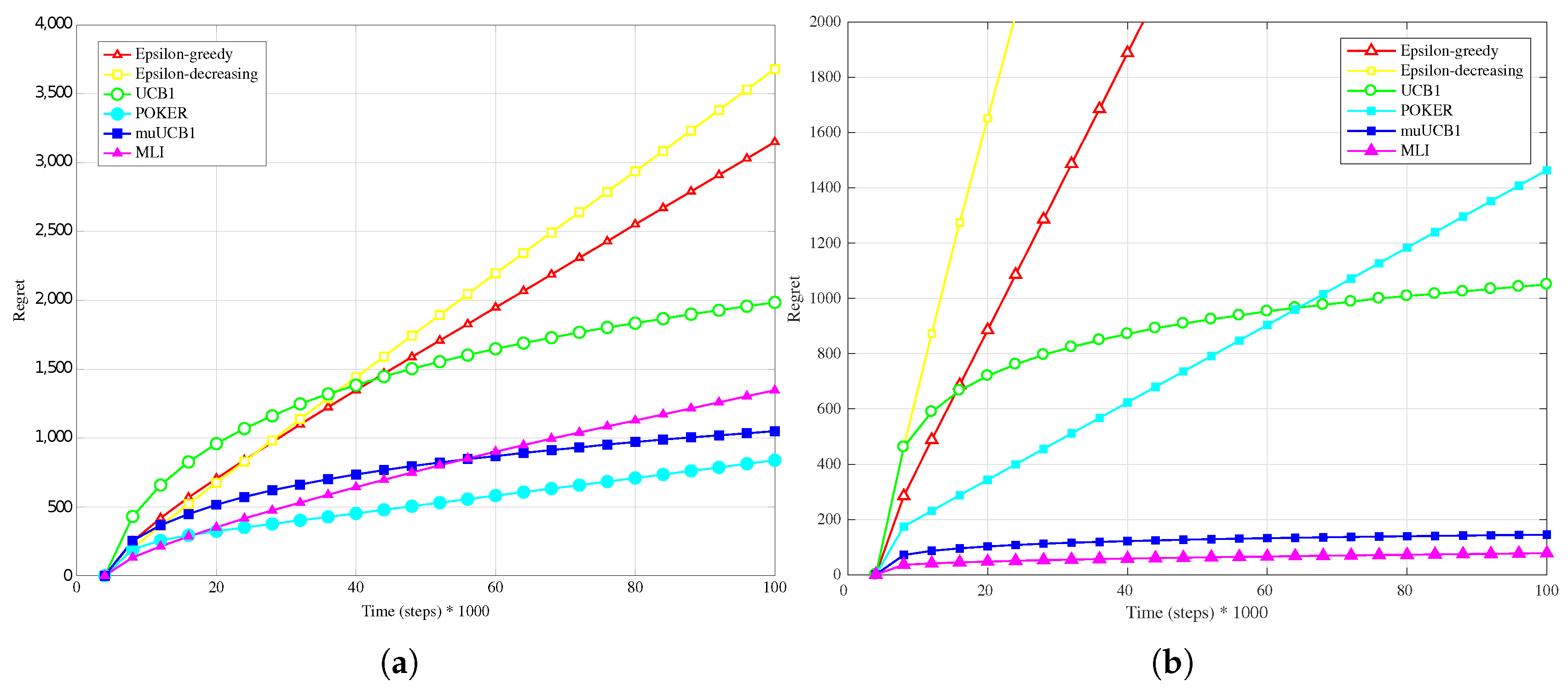
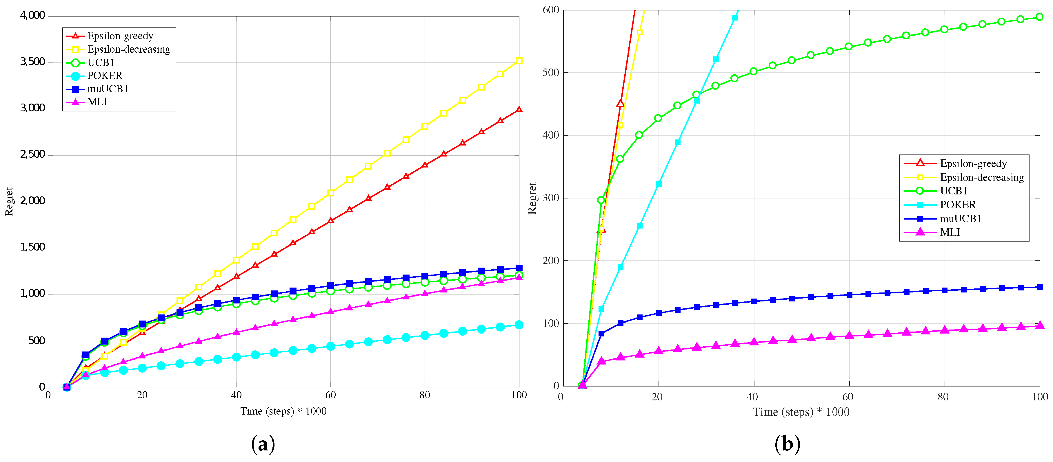
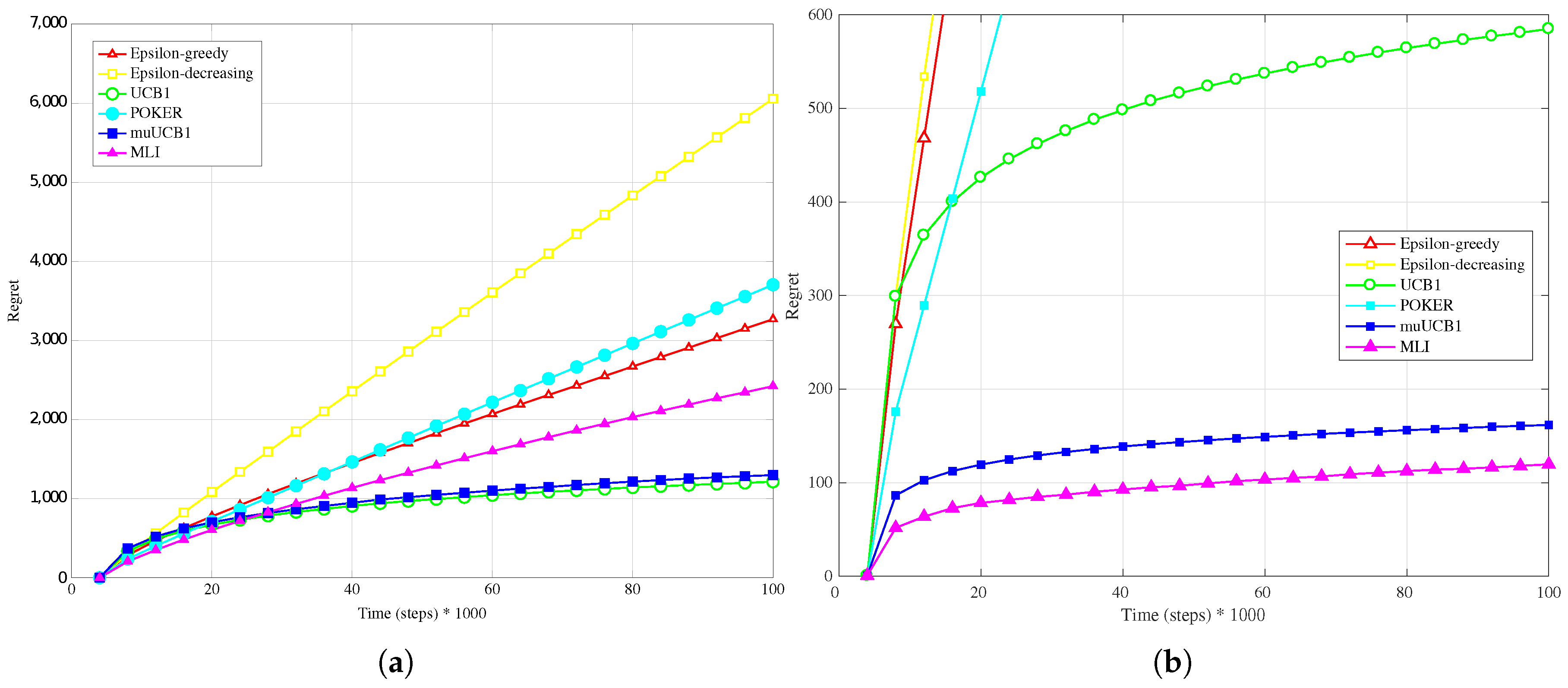
The trend is confirmed as well when the reward PDF has a truncated Gaussian distribution (Figure 4a, Figure 5a and Figure 6a). With the exception of the case $T_U=T_M$, where UCB1 is clearly the best algorithm at the time horizon, the MLI and muUCB1 perform very well. MLI is the best option when $T_U/T_M=5$ and $T_U/T_M=10$, but muUCB1 improves its performance as the $T_U/T_M$ ratio increases, and achieves similar performance to MLI for $T_U/T_M=10$.

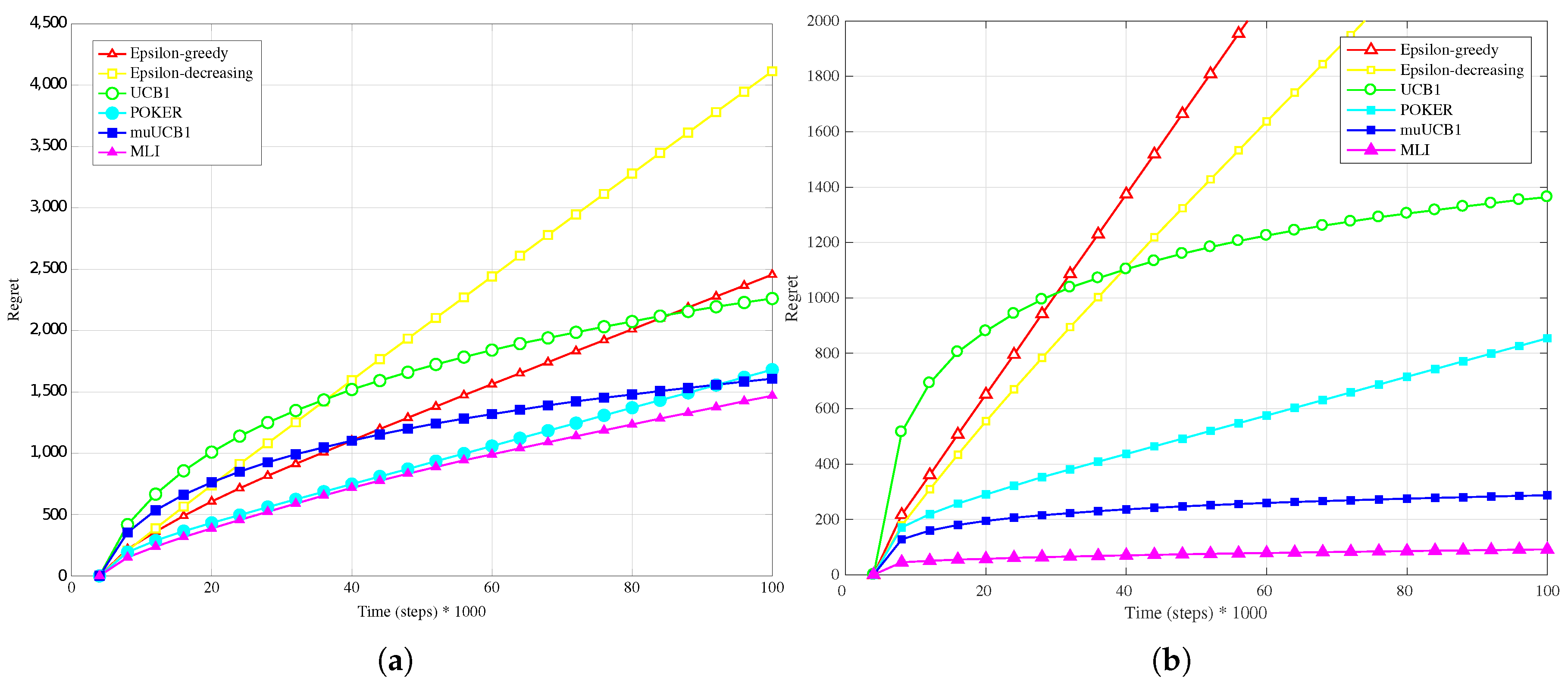
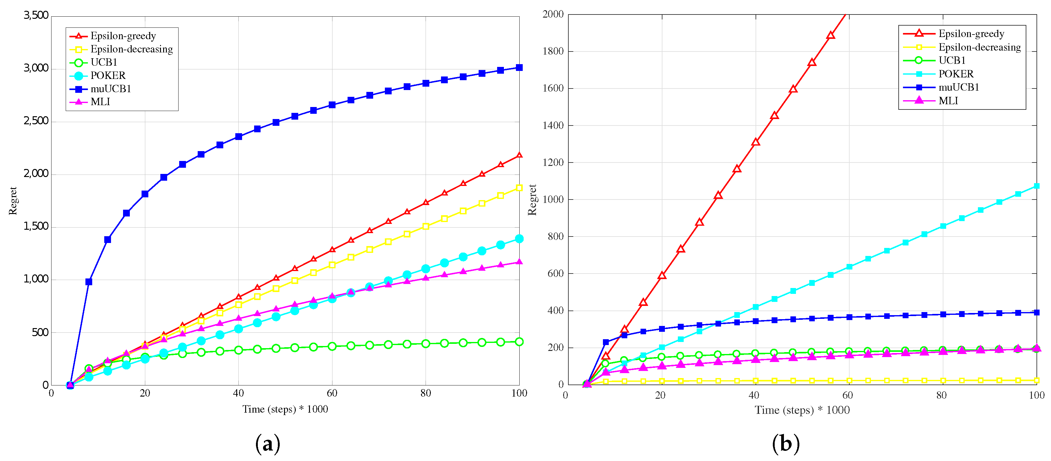
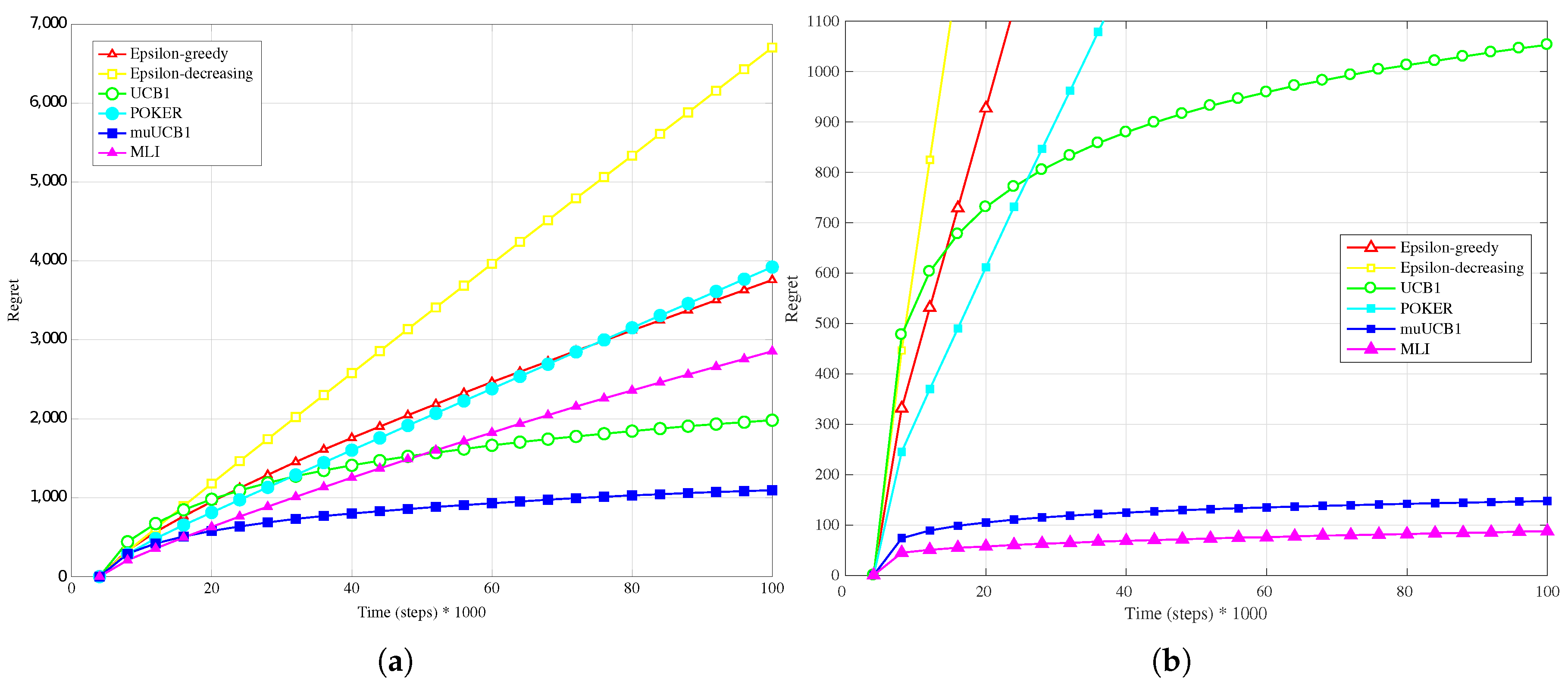
The results obtained with an exponential distribution for the reward PDF, presented in Figure 7a, Figure 8a and Figure 9a, highlight again the performance improvement for muUCB1 as the $T_U/T_M$ ratio increases, leading the new algorithm to be clearly the best option when $T_U/T_M=10$. Notably, the adoption of the exponential distribution has a strong impact on the performance of the POKER algorithm, which presents a linear growth of regret with time; a similar behavior is observed for the MLI algorithm.

As a general comment on the $\epsilon$-greedy and $\epsilon$-decreasing algorithms, not discussed so far, they present a linear growth of regret with time for all considered distributions, and lead in general to the worst performance. The algorithms, that despite their simplicity have shown good results with a classical MAB model [16,17], are thus not suitable for adoption in the new model with the considered PDFs and mean value configuration, in particular as the $T_U/T_M$ ratio grows.

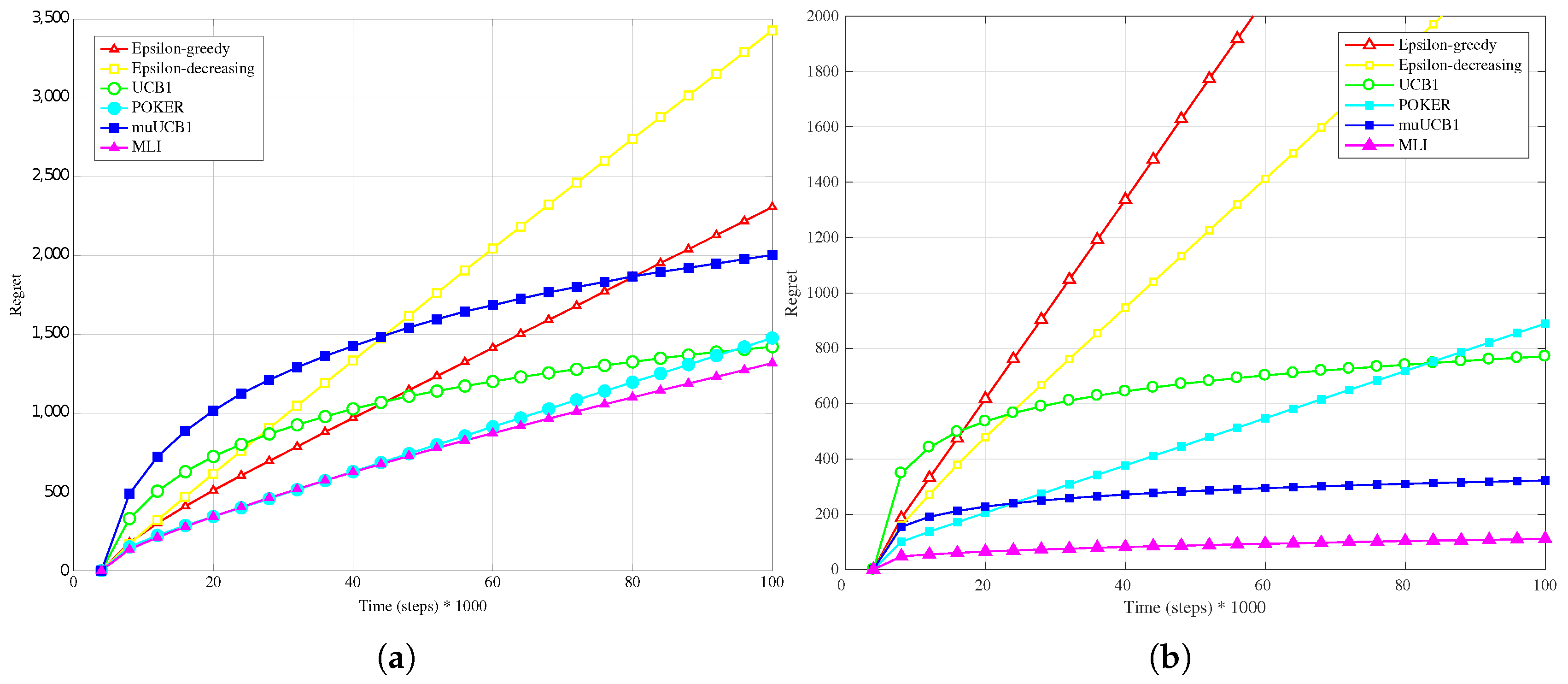
4.2. Synthetic Data-Easy Configuration

Results obtained in the case of the Easy configuration, when one arm is significantly more rewarding than the other ones, are rather different from those observed in Section 4.1 for the Hard configuration. Figure 1b, Figure 2b and Figure 3b, presenting results for the Bernoulli distribution, show that UCB1, muUCB1 and MLI algorithms perform better than in the Hard configuration, while the opposite is true for a second group of algorithms including POKER, $\epsilon$-decreasing and $\epsilon$-greedy, that in most cases lead to a worse performance, in particular as the $T_U/T_M$ ratio increases. These results can be explained by observing that the latter group includes the traditional algorithms that are more aggressive in using the estimated best arm: as a result, they are able to achieve almost the maximum gain when they correctly select the best arm, but incur in a high penalty when they select a sub-optimal arm. Among algorithms in the first group, results show that the gap between muUCB1 and UCB1 is small for $T_U/T_M=1$, and the muUCB1 algorithm performs significantly better than UCB1 when the ratio grows. The performance of the two proposed algorithms is particularly good for $T_U/T_M=10$, with MLI providing the best overall performance.

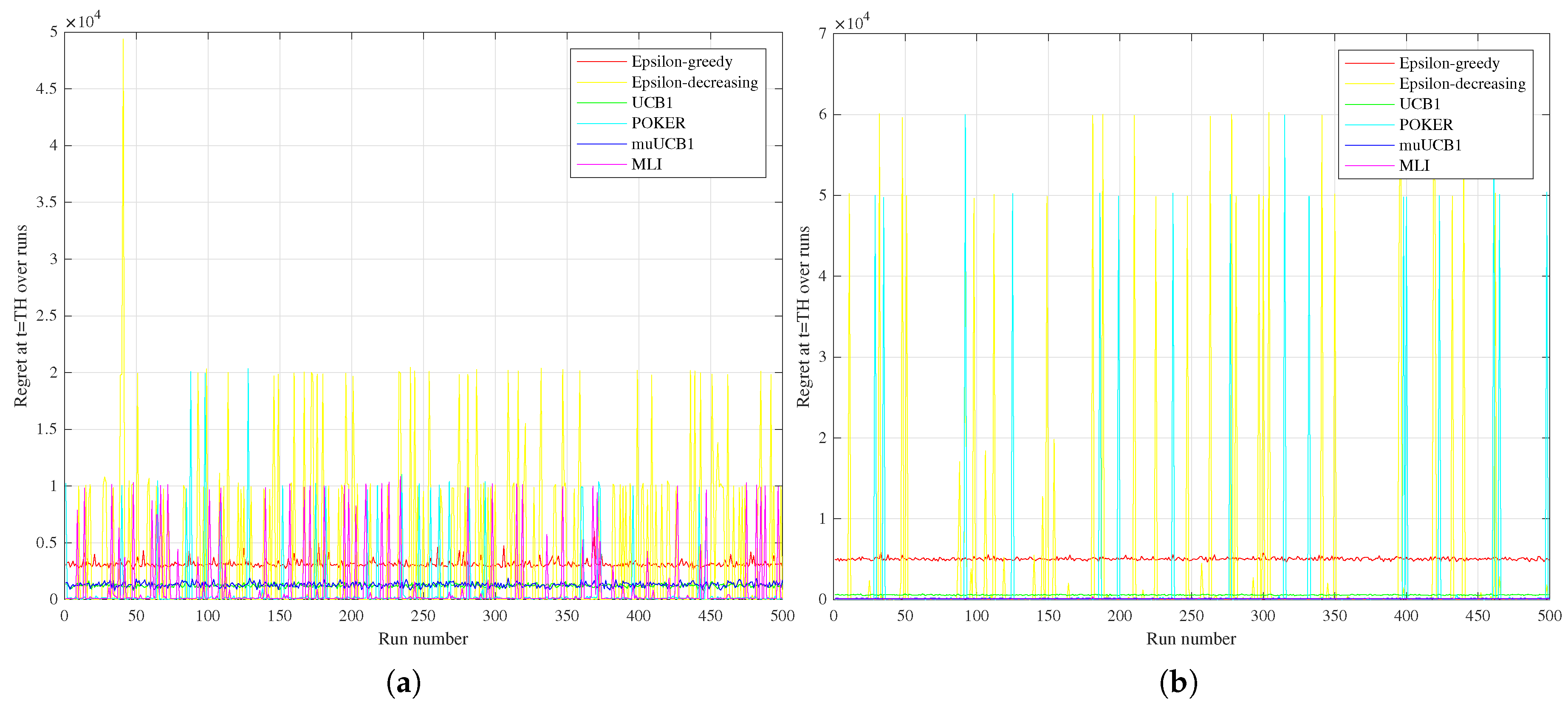
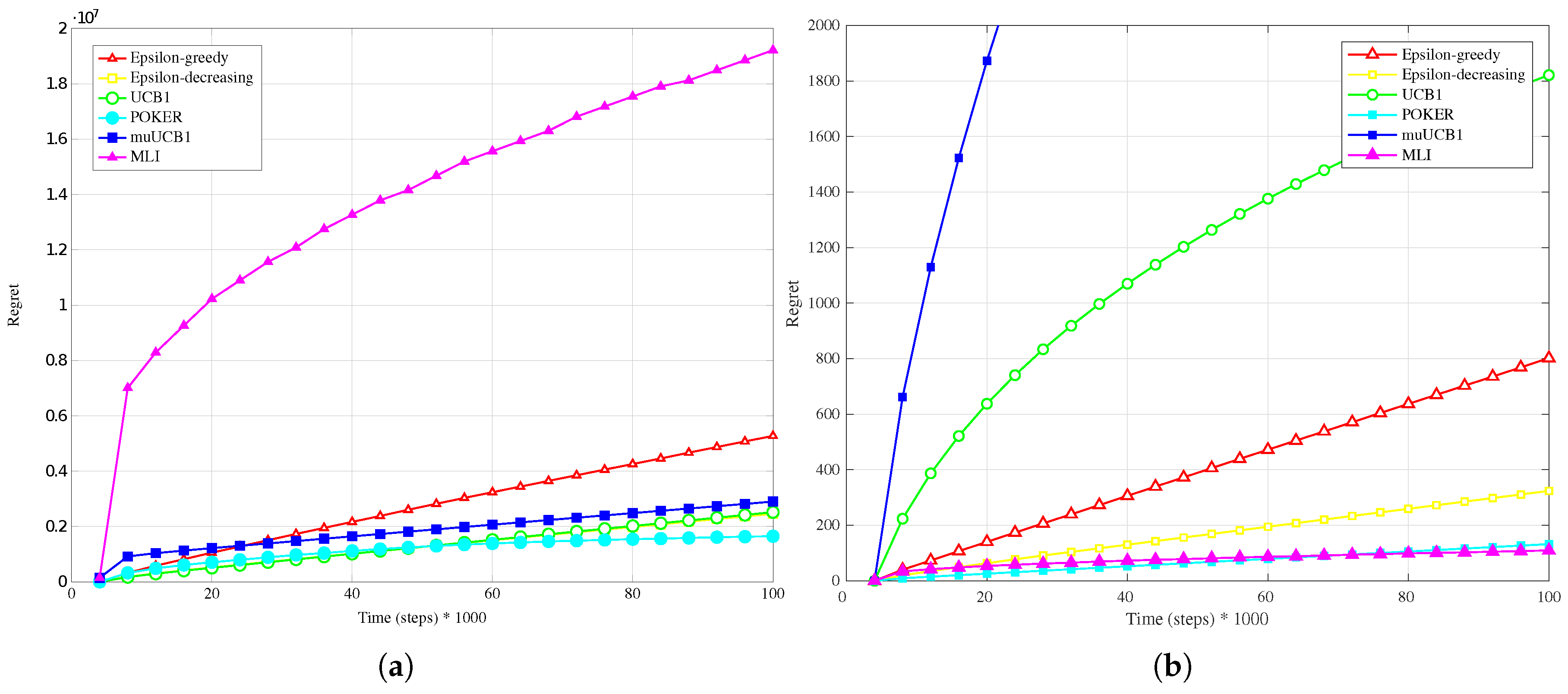
The different performance between the two groups of algorithms can be better understood by observing Figure 10, comparing the regret measured at the time horizon for the six algorithms over the 500 runs for the Bernoulli distribution with $T_U/T_M=5$ in the Hard vs. Easy configurations (Figure 10a vs. Figure 10b, respectively). Results highlight that POKER and $\epsilon$-decreasing algorithms are characterized, both in the Hard and Easy configurations, by several spikes in the regret at the time horizon, corresponding to runs where a sub-optimal arm was selected, leading to linear regret over time. This behavior is observed for MLI as well in the Hard configuration, but disappears in the Easy one, where the algorithm is highly consistent in eventually selecting the best arm in each run.

The results for the truncated Gaussian distribution, presented in Figure 4b, Figure 5b and Figure 6b, show a similar behavior: the performance of UCB1 decreases significantly as $T_U/T_M$ increases, while muUCB1 and MLI show the opposite trend. The POKER, $\epsilon$-decreasing and $\epsilon$-greedy algorithms confirm a high variability in the experienced regret when $T_U/T_M>1$; even in the case $T_U/T_M=1$, the only algorithm in this group that achieves good performance is the $\epsilon$-decreasing.

Finally, results for the exponential distribution, presented in Figure 7b, Figure 8b and Figure 9b, also confirm the behavior observed for the other distributions: MLI and muUCB1 algorithms lead to the best performance, and UCB1 is the only traditional algorithm leading to a logarithmic regret when $T_U/T_M>1$, while $\epsilon$-greedy, $\epsilon$-decreasing and POKER algorithms show a steep linear regret over time.

Overall, results obtained in the Easy configuration show that when an arm provides a significant advantage over the others, traditional algorithms that tend to favor exploitation over exploration, and in particular POKER and $\epsilon$-decreasing, typically perform either extremely well o extremely poorly, depending on the selection of the arm in the early steps.

The proposed algorithms are confirmed to perform better than traditional ones when $T_U/T_M>1$; in this configuration, however, MLI performs better then muUCB1, thanks to its capability of taking advantage of the measure action introduced in the muMAB model, combined with an aggressive approach favoring use over measure. The MLI algorithm is thus the best choice, also in light of its robustness to different reward distributions.

4.3. Real Data-Linear Conversion

Figure 11a, Figure 12a and Figure 13a present results obtained with real data when a linear conversion from latency to reward is adopted. Results show that MLI obtains the worst performance with all the considered $T_U/T_M$ ratios, with a large gap in terms of regret with respect to the other algorithms.

This outcome can be explained by observing that the rewards obtained by linear conversion from the latencies present a large variance; in fact, every Internet web-site home page visited (corresponding to a different wireless network, in the considered scenario) answered with extremely variable latency values. This variability prevents the algorithms to correctly estimate their mean values with few samples. This is particularly true for MLI, which strongly relies for its use actions choices on the estimates built up during the first steps. This is an advantage in scenarios where the measured data do not present such a high variability, as seen in Section 4.2, but leads to a significant performance penalty in the opposite case. Overall, POKER and $\epsilon$-decreasing are the algorithms that provide the most reliable performance, leading to the best results for $T_U/T_M=5$ and $T_U/T_M=10$, respectively.

4.4. Real Data-Logarithmic Conversion

The adoption of the a logarithmic conversion has the effect of significantly reducing the variability of the rewards when compared to the linear conversion analyzed in Section 4.3. This, in turn, has a dramatic impact on the performance of the MLI algorithm. Results presented in Figure 11b, Figure 12b and Figure 13b show in fact that the MLI algorithm leads to a regret in line with the POKER and $\epsilon$-decreasing algorithms, in particular for $T_U/T_M>1$. Oppositely, algorithms that are more conservative in exploiting/using, such as UCB1 and muUCB1, are not capable of taking full advantage of the low variance in rewards; in this case as well, however, the performance of the muUCB1 algorithm improves as $T_U/T_M$ increases.

4.5. Discussion of Results

Results presented in this section clearly show that the best choice on the algorithm to use strongly depends on the distribution of the rewards. Conservative algorithms that spend more time measuring/exploring, such as UCB1 and muUCB1, should be preferred when the different arms are characterized by similar rewards, while the MLI algorithm, more tilted towards use, should be the preferred choice when one arm is significantly better than others. Other aggressive algorithms such as POKER and $\epsilon$-decreasing may potentially lead to an extremely low regret, but present a very high variability in final regret, and are thus characterized by a low reliability.

Results also show that the proposed MLI and muUCB1 algorithms, which are capable of taking advantage of the measuring phase introduced in the muMAB model, consistently improve their performance as the $T_U/T_M$ ratio increases.

Transferring the above observations into real world cases, this means that the choice of which algorithm to use strongly depends on which network quality parameters are taken into account in network selection. As an example, a binary parameter such as the availability of a network can be modelled with a Bernoulli distribution [25], while a parameter such as the measured SNR in a channel affected by Rayleigh fading can be modelled as an exponential random variable [26].

In the considered scenario, where the final goal is to offer the final user the best performance in terms of perceived quality, the parameters of the networks we are interested on depend, in turn, on the type of application that the user wants to use, and therefore on the requested traffic type; models linking measurable network parameters to perceived quality have been indeed proposed in the literature (see, for example, [26]).

Results also allow to observe that the variability of the selected network parameters may play a significant role in the selection of the network selection algorithm: if the reward obtained by the network parameters presents a large variance, some algorithms may incur in a large penalty in terms of regret.

An additional important consideration should be done on the considered time horizon: given the same reward distribution and the same $T_U/T_M$ ratio, two different time horizons can require the selection of different algorithms in order to guarantee the lowest regret. As an a example, MLI during the very first steps only performs measure actions, thus obtaining a null gain. It is, therefore, obvious that if the time horizon is very short, this algorithm should never be selected. In real world scenarios, where it can be expected that the considered time horizon is usually much longer, this initial period can be considered negligible; more details on this aspect can be found in [27]. Again, the definition of the time horizon will, however, depend on the selected network QoS/QoE parameters: if parameters change frequently, this will translate in a short available time horizon, which would call for an algorithm capable of accumulating gain in a shorter time.

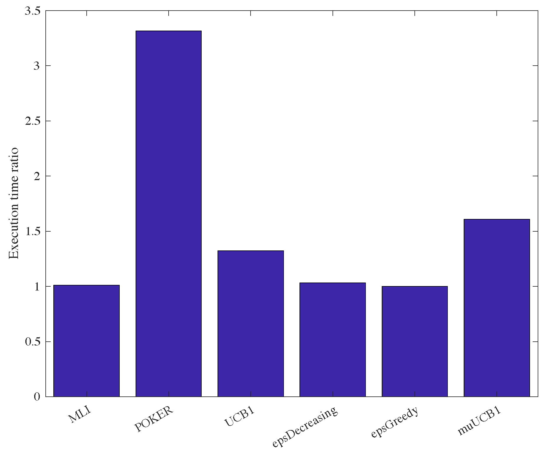
One last aspect worth mentioning regards computational complexity. Although a complete complexity analysis is not carried out in this work, the proposed algorithms were compared with existing ones by measuring the execution time assuming a ratio $T_U/T_M=1$. Results are presented in Figure 14, showing the ratio between the execution time of each algorithm and the execution time of the $\epsilon$-greedy algorithm, which proved to be the fastest one. Results show that $\epsilon$-greedy, $\epsilon$-decreasing and MLI algorithms require similar execution times. The UCB1 and muUCB1 are characterized by a slightly longer execution time, due to added complexity related to the calculation of indexes, while the POKER algorithm is significantly slower, reflecting the higher complexity in the evaluation of the arm to select, as discussed in [17]. A thorough analysis of complexity is planned in a future extension of this work.

5. Conclusions

In this work, a new model for Multi-Armed Bandit problems, referred to as muMAB, was proposed. The model introduces the presence of two different actions: to measure and to use. In addition, the model introduces a gain for measuring vs. using a resource, and the regret, that is the classical parameter for the performance evaluation of MAB algorithms, is updated accordingly, so as to measure the difference between gains. The muMAB model is better suited than classical MAB models to represent real world scenarios, such as the choice of a wireless network among the available ones based on criteria of final user perceived quality maximization.

Two algorithms designed to take into account the higher flexibility allowed by the muMAB model, referred to as muUCB1 and MLI, were also introduced. Their performance was evaluated and compared with the performance obtained by algorithms already present in literature by simulation. The simulations were performed considering different conditions in terms of distributions for the rewards PDF, and values of the ratio between the use period duration and the measure period duration. Results show that there is no optimal choice valid for every case; the algorithm that performs best, i.e., that permits to obtain the lowest regret, depends on the reward PDF and on the $T_U/T_M$ ratio. Moreover, the choice should also depend on the considered time horizon, since different algorithms show a different regret growth rate with time.

Results with synthetic data indicate, in particular, that the muUCB1 algorithm is the best option when arms are characterized by similar rewards, especially for high $T_U/T_M$ ratios, when the time required to measure the performance of each candidate arm is significantly shorter than the time spent using the selected arm before a change is possible. Oppositely, the more aggressive MLI algorithm is the best choice when one arm has a significantly larger reward than the others, in particular, again, for high $T_U/T_M$ ratios.

Future work will investigate this aspect by determining the minimum threshold for $T_U/T_M$ that makes the use of algorithms that alternate measure and use actions advantageous with respect to traditional algorithms that only perform use actions, and will assess the problem of adaptively switching between a conservative algorithm, like muUCB1, and a more aggressive one, like MLI, depending on the current estimate of the rewards provided by the different arms. Future work will also address the issue of scalability of the proposed algorithms, to be considered a key aspect in their application to 5G, given the massive number of devices expected in 5G network scenarios; since the MAB model does not take into account interaction between users, this aspect can be introduced by adopting a definition of the reward that is influenced by the behavior and by the selection of other users; a glimpse of this kind of analysis can be found in [19]. An extension of this work will focus on applying the proposed MAB model to real world scenarios related to wireless network selection in a multi-RAT environment, in order to quantitatively assess its accuracy in combination with different utility metrics to be adopted as reward, including those impacted by user interaction.