Single Machine Scheduling Problem with Interval Processing Times and Total Completion Time Objective

Abstract

We consider a single machine scheduling problem with uncertain durations of the given jobs. The objective function is minimizing the sum of the job completion times. We apply the stability approach to the considered uncertain scheduling problem using a relative perimeter of the optimality box as a stability measure of the optimal job permutation. We investigated properties of the optimality box and developed algorithms for constructing job permutations that have the largest relative perimeters of the optimality box. Computational results for constructing such permutations showed that they provided the average error less than $0.74\%$ for the solved uncertain problems.

1. Introduction

Since real-life scheduling problems involve different forms of uncertainties, several approaches have been developed in the literature for dealing with uncertain scheduling problems. In a stochastic approach, job processing times are assumed to be random variables with the known probability distributions [1,2]. If one has no sufficient information to characterize the probability distribution of all random processing times, other approaches are needed [3,4,5]. In the approach of seeking a robust schedule [3,6], the decision-maker prefers a schedule that hedges against the worst-case scenario. A fuzzy approach [7,8,9] allows a scheduler to determine best schedules with respect to fuzzy processing times. A stability approach [10,11,12] is based on the stability analysis of the optimal schedules to possible variations of the numerical parameters. In this paper, we apply the stability approach to a single machine scheduling problem with uncertain processing times of the given jobs. In Section 2, we present the setting of the problem and the related results. In Section 3, we investigate properties of an optimality box of the permutation used for processing the given jobs. Efficient algorithms are derived for finding a job permutation with the largest relative perimeter of the optimality box. In Section 5, we develop an algorithm for finding an approximate solution for the uncertain scheduling problem. In Section 6, we report on the computational results for finding the approximate solutions for the tested instances. Section 7 includes the concluding remarks.

2. Problem Setting and the Related Results

There are given n jobs $\mathcal{J}=\{J_1,J_2,...,J_n\}$ to be processed on a single machine. The processing time $p_i$ of the job $J_i\in \mathcal{J}$ can take any real value from the given segment $[p_i^L,p_i^U]$, where $p_i^U\ge p_i^L>0$. The exact value $p_i\in [p_i^L,p_i^U]$ of the job processing time remains unknown until completing the job $J_i\in \mathcal{J}$. Let $R_{+}^n$ denote a set of all non-negative n-dimensional real vectors. The set of all possible vectors $(p_1,p_2,\dots ,p_n)=p\in R_{+}^n$ of the job processing times is presented as the Cartesian product of the segments $[p_i^L,p_i^U]$: $T=\{p\in R_{+}^n:p_i^L\le p_i\le p_i^U,i\in \{1,2,\dots ,n\}\}=[p_1^L,p_1^U]\times [p_2^L,p_2^U]\times \dots \times [p_n^L,p_n^U]=:{\times }_{i=1}^n[p_i^L,p_i^U]$. Each vector $p\in T$ is called a scenario.

Let $S=\{{\pi }_1,{\pi }_2,\dots ,{\pi }_{n!}\}$ be a set of all permutations ${\pi }_k=(J_{k_1},$$J_{k_2},\dots ,J_{k_n})$ of the jobs $\mathcal{J}$. Given a scenario $p\in T$ and a permutation ${\pi }_k\in S$, let $C_i=C_i({\pi }_k,p)$ denote the completion time of the job $J_i\in \mathcal{J}$ in the schedule determined by the permutation ${\pi }_k$. The criterion $\sum C_i$ denotes the minimization of the sum of job completion times: ${\sum }_{J_i\in \mathcal{J}}{C}_i({\pi }_t,p)={min}_{{\pi }_k\in S}\left\{{\sum }_{J_i\in \mathcal{J}}{C}_i({\pi }_k,p)\right\},$ where the permutation ${\pi }_t=(J_{t_1},J_{t_2},\dots ,$$J_{t_n})\in S$ is optimal for the criterion $\sum C_i$. This problem is denoted as $1|p_i^L\le p_i\le p_i^U|\sum C_i$ using the three-field notation $\alpha \left|\beta \right|\gamma$ [13], where $\gamma$ denotes the objective function. If scenario $p\in T$ is fixed before scheduling, i.e., $[p_i^L,p_i^U]=[p_i,p_i]$ for each job $J_i\in \mathcal{J}$, then the uncertain problem $1|p_i^L\le p_i\le p_i^U|\sum C_i$ is turned into the deterministic one $1\left|\right|\sum C_i$. We use the notation $1\left|p\right|\sum C_i$ to indicate an instance of the problem $1\left|\right|\sum C_i$ with the fixed scenario $p\in T$. Any instance $1\left|p\right|\sum C_i$ is solvable in $O(nlogn)$ time [14] since the following claim has been proven.

Theorem 1.

The job permutation ${\pi }_k=(J_{k_1},J_{k_2},\dots ,J_{k_n})\in S$ is optimal for the instance $1\left|p\right|\sum C_i$ if and only if the following inequalities hold: $p_{k_1}\le p_{k_2}\le \dots \le p_{k_n}$. If $p_{k_u}<p_{k_v}$, then job $J_{k_u}$ precedes job $J_{k_v}$ in any optimal permutation ${\pi }_k$.

Since a scenario $p\in T$ is not fixed for the uncertain problem $1|p_i^L\le p_i\le p_i^U|\sum C_i$, the completion time $C_i$ of the job $J_i\in \mathcal{J}$ cannot be exactly determined for the permutation ${\pi }_k\in S$ before the completion of the job $J_i$. Therefore, the value of the objective function $\sum C_i$ for the permutation ${\pi }_k$ remains uncertain until jobs $\mathcal{J}$ have been completed.

Definition 1.

Job $J_v$ dominates job $J_w$ (with respect to T) if there is no optimal permutation ${\pi }_k\in S$ for the instance $1\left|p\right|\sum C_i$, $p\in T$, such that job $J_w$ precedes job $J_v$.

The following criterion for the domination was proven in [15].

Theorem 2.

Job $J_v$ dominates job $J_w$ if and only if $p_v^U<p_w^L$.

Since for the problem $\alpha |p_i^L\le p_i\le p_i^U|\gamma$, there does not usually exist a permutation of the jobs $\mathcal{J}$ being optimal for all scenarios T, additional objectives or agreements are often used in the literature. In particular, a robust schedule minimizing the worst-case regret to hedge against data uncertainty has been developed in [3,8,16,17,18,19,20]. For any permutation ${\pi }_k\in S$ and any scenario $p\in T$, the difference ${\gamma }_p^k-{\gamma }_p^t=:r({\pi }_k,p)$ is called the regret for permutation ${\pi }_k$ with the objective function $\gamma$ equal to ${\gamma }_p^k$ under scenario p. The value $Z\left({\pi }_k\right)=max\{r({\pi }_k,p):p\in T\}$ is called the worst-case absolute regret. The value $Z^{*}\left({\pi }_k\right)=max\{\frac{r({\pi }_k,p)}{{\gamma }_p^t}:p\in T\}$ is called the worst-case relative regret. While the deterministic problem $1\left|\right|\sum C_i$ is polynomially solvable [14], finding a permutation ${\pi }_t\in S$ minimizing the worst-case absolute regret $Z\left({\pi }_k\right)$ or the relative regret $Z^{*}\left({\pi }_k\right)$ for the problem $1|p_i^L\le p_i\le p_i^U|\sum C_i$ are binary NP-hard even for two scenarios [19,21]. In [6], a branch-and-bound algorithm was developed to find a permutation ${\pi }_k$ minimizing the absolute regret for the problem $1|p_i^L\le p_i\le p_i^U|\sum w_i{C}_i$, where jobs $J_i\in \mathcal{J}$ have weights $w_i>0$. The computational experiments showed that the developed algorithm is able to find such a permutation ${\pi }_k$ for the instances with up to 40 jobs. The fuzzy scheduling technique was used in [7,8,9,22] to develop a fuzzy analogue of dispatching rules or to solve mathematical programming problems to determine a schedule that minimizes a fuzzy-valued objective function.

In [23], several heuristics were developed for the problem $1|p_i^L\le p_i\le p_i^U|\sum w_i{C}_i$. The computational experiments including different probability distributions of the processing times showed that the error of the best performing heuristic was about $1\%$ of the optimal objective function value $\sum w_i{C}_i$ obtained after completing the jobs when their factual processing times became known.

The stability approach [5,11,12] was applied to the problem $1|p_i^L\le p_i\le p_i^U|\sum w_i{C}_i$ in [15], where hard instances were generated and solved by the developed Algorithm MAX-OPTBOX with the average error equal to $1.516783\%$. Algorithm MAX-OPTBOX constructs a job permutation with the optimality box having the largest perimeter.

In Section 3, Section 4, Section 5 and Section 6, we continue the investigation of the optimality box for the problem $1|p_i^L\le p_i\le p_i^U|\sum C_i$. The proven properties of the optimality box allows us to develop Algorithm 2 for constructing a job permutation with the optimality box having the largest relative perimeter and Algorithm 3, which outperforms Algorithm MAX-OPTBOX for solving hard instances of the problem $1|p_i^L\le p_i\le p_i^U|\sum C_i$. Algorithm 3 constructs a job permutation ${\pi }_k$, whose optimality box provides the minimal value of the error function introduced in Section 5. Randomly generated instances of the problem $1|p_i^L\le p_i\le p_i^U|\sum C_i$ were solved by Algorithm 3 with the average error equal to $0.735154\%$.

3. The Optimality Box

Let M denote a subset of the set $N=\{1,2,\dots ,n\}$. We define an optimality box for the job permutation ${\pi }_k\in S$ for the problem $1|p_i^L\le p_i\le p_i^U|\sum C_i$ as follows.

Definition 2.

The maximal (with respect to the inclusion) rectangular box $\mathcal{OB}({\pi }_k,T)={\times }_{k_i\in M}[l_{k_i}^{*},u_{k_i}^{*}]\subseteq T$ is called the optimality box for the permutation ${\pi }_k=(J_{k_1},J_{k_2},\dots ,J_{k_n})\in S$ with respect to $T,$ if the permutation ${\pi }_k$ being optimal for the instance $1\left|p\right|\sum C_i$ with the scenario $p=(p_1,p_2,\dots ,p_n)\in T$ remains optimal for the instance $1|p^{\prime }|\sum C_i$ with any scenario $p^{\prime }\in \mathcal{OB}({\pi }_k,T)\times \left\{{\times }_{k_j\in N\backslash M}[p_{k_j},p_{k_j}]\right\}$. If there does not exist a scenario $p\in T$ such that the permutation ${\pi }_k$ is optimal for the instance $1\left|p\right|\sum C_i$, then $\mathcal{OB}({\pi }_k,T)=\varnothing$.

Any variation $p_{k_i}^{\prime }$ of the processing time $p_{k_i}$, $J_{k_i}\in \mathcal{J}$, within the maximal segment $[l_{k_i}^{*},u_{k_i}^{*}]$ indicated in Definition 2 cannot violate the optimality of the permutation ${\pi }_k\in S$ provided that the inclusion $p_{k_i}^{\prime }\in [l_{k_i}^{*},u_{k_i}^{*}]$ holds. The non-empty maximal segment $[l_{k_i}^{*},u_{k_i}^{*}]$ with the inequality $l_{k_i}^{*}\le u_{k_i}^{*}$ and the length $u_{k_i}^{*}-l_{k_i}^{*}\ge 0$ indicated in Definition 2 is called an optimality segment for the job $J_{k_i}\in \mathcal{J}$ in the permutation ${\pi }_k$. If the maximal segment $[l_{k_i}^{*},u_{k_i}^{*}]$ is empty for job $J_{k_i}\in \mathcal{J}$, we say that job $J_{k_i}$ has no optimality segment in the permutation ${\pi }_k$. It is clear that if job $J_{k_i}$ has no optimality segment in the permutation ${\pi }_k$, then the inequality $l_{k_i}^{*}>u_{k_i}^{*}$ holds.

3.1. An Example of the Problem $1|p_i^L\le p_i\le p_i^U|\sum C_i$

Following to [15], the notion of a block for the jobs $\mathcal{J}$ may be introduced for the problem $1|p_i^L\le p_i\le p_i^U|\sum C_i$ as follows.

Definition 3.

A maximal set $B_r=\{J_{r_1},J_{r_2},\dots ,J_{r_{|B_r|}}\}\subseteq \mathcal{J}$ of the jobs, for which the inequality ${max}_{J_{r_i}\in B_r}{p}_{r_i}^L\le {min}_{J_{r_i}\in B_r}{p}_{r_i}^U$ holds, is called ablock. The segment $[b_r^L,b_r^U]$ with $b_r^L={max}_{J_{r_i}\in B_r}{p}_{r_i}^L$ and $b_r^U={min}_{J_{r_i}\in B_r}{p}_{r_i}^U$ is called acoreof the block $B_r$.

If job $J_i\in \mathcal{J}$ belongs to only one block, we say that job $J_i$ is fixed (in this block). If job $J_k\in \mathcal{J}$ belongs to two or more blocks, we say that job $J_k$ is non-fixed. We say that the block $B_v$ is virtual, if there is no fixed job in the block $B_v$.

Remark 1.

Any permutation ${\pi }_k\in S$ determines a distribution of all non-fixed jobs to their blocks. Due to the fixings of the positions of the non-fixed jobs, some virtual blocks may be destroyed for the permutation ${\pi }_k$. Furthermore, the cores of some non-virtual blocks may be increased in the permutation ${\pi }_k$.

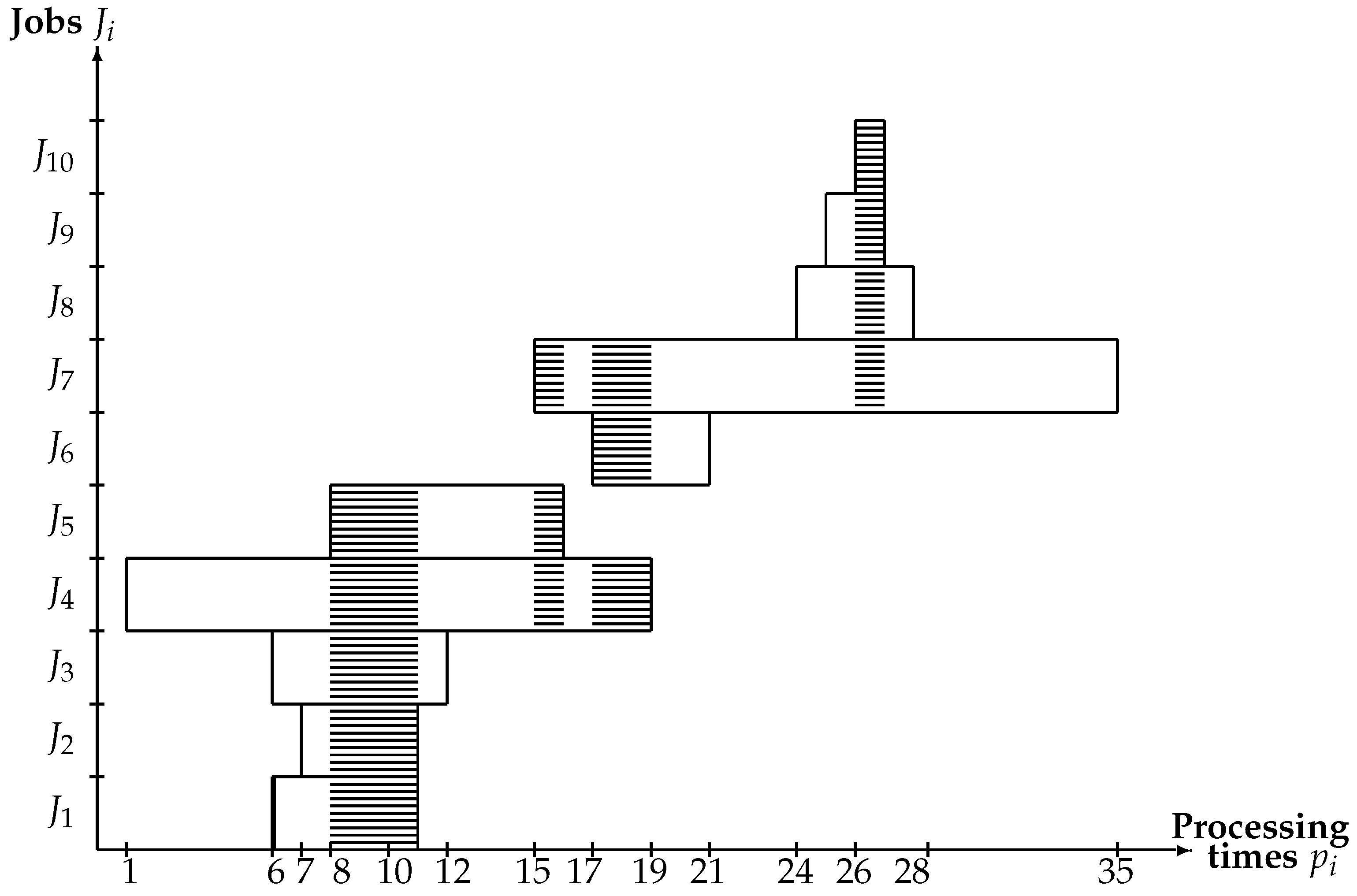
We demonstrate the above notions on a small example with input data given in Table 1. The segments $[p_i^L,p_i^U]$ of the job processing times are presented in a coordinate system in Figure 1, where the abscissa axis is used for indicating the segments given for the job processing times and the ordinate axis for the jobs from the set $\mathcal{J}$. The cores of the blocks $B_1$, $B_2$, $B_3$ and $B_4$ are dashed in Figure 1.

Table 1. Input data for the problem $1|p_i^L\le p_i\le p_i^U|\sum C_i$.

i	1	2	3	4	5	6	7	8	9	10
$p_i^L$	6	7	6	1	8	17	15	24	25	26
$p_i^U$	11	11	12	19	16	21	35	28	27	27

Figure 1. The segments $[p_i^L,p_i^U]$ given for the feasible processing times of the jobs $J_i\in \mathcal{J}=\{J_1,J_2,\dots ,J_{10}\}$ (the cores of the blocks $B_1$, $B_2$, $B_3$ and $B_4$ are dashed).

There are four blocks in this example as follows: $\{B_1,B_2,B_3,B_4\}=:B$. The jobs $J_1$, $J_2$, $J_3$, $J_4$ and $J_5$ belong to the block $B_1$. The jobs $J_4$, $J_5$ and $J_7$ are non-fixed. The remaining jobs $J_1$, $J_2$, $J_3$, $J_6$, $J_8$, $J_9$ and $J_{10}$ are fixed in their blocks. The block $B_2$ is virtual. The jobs $J_4$, $J_5$ and $J_7$ belong to the virtual block $B_2$. The jobs $J_4$, $J_6$, and $J_7$ belong to the block $B_3$. The jobs $J_7$, $J_8$, $J_9$ and $J_{10}$ belong to the block $B_4$.

3.2. Properties of a Job Permutation Based on Blocks

The proof of Lemma 1 is based on Procedure 1.

Lemma 1.

For the problem $1|p_i^L\le p_i\le p_i^U|\sum C_i$, the set $B=\{B_1,B_2,\dots ,B_m\}$ of all blocks can be determined in $O(nlogn)$ time.

Proof. 

The right bound $b_1^U$ of the core of the first block $B_1\in B$ is determined as follows: $b_1^U={min}_{J_i\in \mathcal{J}}{p}_i^U$. Then, all jobs included in the block $B_1$ may be determined as follows: $B_1=\{J_i\in \mathcal{J}:p_i^L\le b_1^U\le p_i^U\}$. The left bound $b_1^L$ of the core of the block $B_1$ is determined as follows: $b_1^L={max}_{J_i\in B_1}{p}_i^L$. Then, one can determine the second block $B_2\in B$ via applying the above procedure to the subset of set $\mathcal{J}$ without jobs $J_i$, for which the equality $b_1^U=p_i^U$ holds. This process is continued until determining the last block $B_m\in B$. Thus, one can use the above procedure (we call it Procedure 1) for constructing the set $B=\{B_1,B_2,\dots ,B_m\}$ of all blocks for the problem $1|p_i^L\le p_i\le p_i^U|\sum C_i$. Obviously, Procedure 1 has the complexity $O(nlogn)$. ☐

Any block from the set B has the following useful property.

Lemma 2.

At most two jobs in the block $B_r\in B$ may have the non-empty optimality segments in any fixed permutation ${\pi }_k\in S$.

Proof. 

Due to Definition 3, the inclusion $[b_r^L,b_r^U]\subseteq [p_i^L,p_i^U]$ holds for each job $J_i\in B_r$. Thus, due to Definition 2, only job $J_{k_i}$, which is the first one in the permutation ${\pi }_k$ among the jobs from the block $B_r$, and only job $J_{k_v}\in B_r$, which is the last one in the permutation ${\pi }_k$ among the jobs from the block $B_r$, may have the non-empty optimality segments. It is clear that these non-empty segments look as follows: $[p_{k_i}^L,u_{k_i}^{*}]$ and $[l_{k_v}^{*},p_{k_v}^U]$, where $u_{k_i}^{*}\le b_r^L$ and $b_r^U\le l_{k_v}^{*}$. ☐

Lemma 3.

If $\mathcal{OB}({\pi }_k,T)\ne \varnothing$, then any two jobs $J_v\in B_r$ and $J_w\in B_s$, which are fixed in different blocks, $r<s$, must be ordered in the permutation ${\pi }_k\in S$ with the increasing of the left bounds (and the right bounds as well) of the cores of their blocks, i.e., the permutation ${\pi }_k$ looks as follows: ${\pi }_k=(\dots ,J_v,\dots ,J_w,\dots )$, where $b_r^L<b_s^L$.

Proof. 

For any two jobs $J_v\in B_r$ and $J_w\in B_s$, $r<s$, the condition $[p_v^L,p_v^U]\cap [p_w^L,p_w^U]=\varnothing$ holds. Therefore, the same permutation ${\pi }_k=(\dots ,J_v,\dots ,J_w,\dots )$ is obtained if jobs $J_v\in B_r$ and $J_w\in B_s$ are ordered either in the increasing of the left bounds of the cores of their blocks or in the increasing of the right bounds of the cores of their blocks. We prove Lemma 3 by a contradiction. Let the condition $\mathcal{OB}({\pi }_k,T)\ne \varnothing$ hold. However, we assume that there are fixed jobs $J_v\in B_r$ and $J_w\in B_s$, $r<s,$ which are located in the permutation ${\pi }_k\in S$ in the decreasing order of the left bounds of the cores of their blocks $B_r$ and $B_s$. Note that blocks $B_r$ and $B_s$ cannot be virtual.

Due to our assumption, the permutation ${\pi }_k$ looks as follows: ${\pi }_k=(\dots ,J_w,\dots ,J_v,\dots )$, where $b_r^L<b_s^L$. Using Definition 3, one can convince that the cores of any two blocks have no common point. Thus, the inequality $b_r^L<b_s^L$ implies the inequality $b_r^U<b_s^L$. The inequalities $p_v^L\le p_v\le b_r^U<b_s^L\le p_w^L\le p_w$ hold for any feasible processing time $p_v$ and any feasible processing time $p_w$, where $p\in T$. Hence, the inequality $p_v<p_w$ holds as well, and due to Theorem 1, the permutation ${\pi }_k\in S$ cannot be optimal for any fixed scenario $p\in T$. Thus, the equality $\mathcal{OB}({\pi }_k,T)=\varnothing$ holds due to Definition 2. This contradiction with our assumption completes the proof. ☐

Next, we assume that blocks in the set $B=\{B_1,B_2,\dots ,B_m\}$ are numbered according to the increasing of the left bounds of their cores, i.e., the inequality $b_v^L<b_u^L$ implies $v<u$. Due to Definition 3, each block $B_r=\{J_{r_1},J_{r_2},\dots ,J_{r_{|B_r|}}\}$ may include jobs of the following four types. If $p_{r_i}^L=b_r^L$ and $p_{r_i}^U=b_r^U$, we say that job $J_{r_i}$ is a core job in the block $B_r$. Let $B_r^{*}$ be a set of all core jobs in the block $B_r$. If $p_{r_i}^L<b_r^L$, we say that job $J_{r_i}$ is a left job in the block $B_r$. If $p_{r_i}^U>b_r^U$, we say that job $J_{r_i}$ is a right job in the block $B_r$. Let $B_r^{-}$ ($B_r^{+}$) be a set of all left (right) jobs in the block $B_r$. Note that some job $J_{r_i}\in B_r$ may be left-right job in the block $B_r$, since it is possible that $B\backslash \{B_r^{*}\cup B_r^{-}\cup B_r^{+}\}\ne \varnothing$.

Two jobs $J_v$ and $J_w$ are identical if both equalities $p_v^L=p_w^L$ and $p_v^U=p_w^U$ hold. Obviously, if the set $B_r\in B$ is a singleton, $|B_r|=1$, then the equality $B_r=B_r^{*}$ holds. Furthermore, the latter equality cannot hold for a virtual block $B_t\in B$ since any trivial block must contain at least two non-fixed jobs.

Theorem 3.

For the problem $1|p_i^L\le p_i\le p_i^U|\sum C_i$, any permutation ${\pi }_k\in S$ has an empty optimality box $\mathcal{OB}({\pi }_k,T)=\varnothing$, if and only if for each block $B_r\in B$, either condition $|B_r|=|B_r^{*}|\ge 2$ holds or $B_r=B_r^{-}\cup B_r^{+},$ all jobs in the set $B_r^{-}$ (in the set $B_r^{+}$) are identical and the following inequalities hold: $|B_r^{-}|\ge 2$ and $|B_r^{+}|\ge 2$.

Proof. 

Sufficiency. It is easy to prove that there is no virtual block in the considered set B. First, we assume that for each block $B_r\in B$, the condition $|B_r|=|B_r^{*}|\ge 2$ holds.

Due to Lemma 3, in the permutation ${\pi }_k\in S$ with the non-empty optimality box $\mathcal{OB}({\pi }_k,T)\ne \varnothing$, all jobs must be located in the increasing order of the left bounds of the cores of their blocks. However, in the permutation ${\pi }_k\in S$, the following two equalities hold for each block $B_r\in B$: ${min}_{J_i\in B_r}{p}_i^U={max}_{J_i\in B_r}{p}_i^U$ and ${max}_{J_i\in B_r}{p}_i^L={min}_{J_i\in B_r}{p}_i^L.$ Since $|B_r|\ge 2$, there is no job $J_v\in B_r$, which has an optimality segment in any fixed permutation ${\pi }_k\in S$ due to Lemma 2. Hence, the equality $\mathcal{OB}({\pi }_k,T)=\varnothing$ must hold, if the condition $|B_r|=|B_r^{*}|\ge 2$ holds for each block $B_r\in B$.

We assume that there exists a block $B_r\in B$ such that all jobs are identical in the set $B_r^{-}$ with $|B_r^{-}|\ge 2$ and all jobs are identical in the set $B_r^{+}$ with $|B_r^{+}|\ge 2$. Thus, for the permutation ${\pi }_k\in S$, the equalities ${min}_{J_i\in B_r^{-}}{p}_i^U={max}_{J_i\in B_r^{-}}{p}_i^U$ and ${max}_{J_i\in B_r^{-}}{p}_i^L={min}_{J_i\in B_r^{-}}{p}_i^L$ hold. Since $|B_r^{-}|\ge 2$ and all jobs are identical in the set $B_r^{-}$, there is no job $J_v\in B_r^{-}$, which has the optimality segment in any fixed permutation ${\pi }_k\in S$.

Similarly, one can prove that there is no job $J_v\in B_r^{+}$, which has the optimality segment in any fixed permutation ${\pi }_k\in S$. Thus, we conclude that if the condition of Theorem 3 holds for each block $B_r\in B$, then each job $J_i\in \mathcal{J}$ has no optimality segment in any fixed permutation ${\pi }_k\in S$. Thus, if the condition of Theorem 3 holds, the equality $\mathcal{OB}({\pi }_k,T)=\varnothing$ holds for any permutation ${\pi }_k\in S$.

Necessity. We prove the necessity by a contradiction. We assume that any permutation ${\pi }_k\in S$ has an empty optimality box $\mathcal{OB}({\pi }_k,T)=\varnothing$. Let the condition $|B_r|=|B_r^{*}|\ge 2$ do not hold. If $|B_r|=|B_r^{*}|=1$, the set $B_r$ is a singleton and so job $J_{r_1}\in B_r$ has the optimality segment $[p_{r_1}^L,p_{r_1}^U]$ with the length $p_{r_1}^U-p_{r_1}^L\ge 0$ in the permutation ${\pi }_{k^{*}}\in S$, where all jobs are ordered according to the increasing of the left bounds of the cores of their blocks. Let the following condition hold:

$$|B_r|>|B_r^{*}|\ge 2.$$

(1)

The condition (1) implies that there exists at least one left job or right job or left-right job $J_{r_i}\in B_r$. If job $J_{r_i}$ is a left job or a left-right job (a right job) in the block $B_r$, then job $J_{r_i}$ must be located on the first place (on the last place, respectively) in the above permutation ${\pi }_{k^{*}}\in S$ among all jobs from the block $B_r$. All jobs from the set $B_r\backslash \{B_r^{*}\cup \left\{J_{r_i}\right\}\}$ must be located between job $J_{r_v}\in B_r^{*}$ and job $J_{r_w}\in B_r^{*}$. Therefore, the left job $J_{r_i}$ or the left-right job $J_{r_i}$ (the right job $J_{r_i}$) has the following optimality segment $[p_{r_i}^L,b_r^L]$ (segment $[b_r^U,p_{r_i}^U]$, respectively) with the length $b_r^L-p_{r_i}^L>0$ (the length $p_{r_i}^U-b_r^U>0$, respectively) in the permutation ${\pi }_{k^{*}}$. Let the equality $B_r=B_r^{-}\cup B_r^{+}$ do not hold. If there exist a job $J_{r_i}\in B_r^{*}$, this job must be located between the jobs $J_{r_v}\in B_r^{-}$ and $J_{r_w}\in B_r^{-}$. It is clear that the job $J_{r_i}$ has the optimality segment $[b_r^L,b_r^U]$ with the length $b_r^U-b_r^L>0$ in the permutation ${\pi }_{k^{*}}$.

Let the following conditions hold: $B_r=B_r^{-}\cup B_r^{+}$, $|B_r^{-}|\ge 2$, $|B_r^{+}|\ge 2$. However, we assume that jobs from the set $B_r^{-}$ are not identical. Then the job $J_{r_u}\in B_r^{-}$ with the largest segment $[p_{r_u}^L,p_{r_u}^U]$ among the jobs from the set $B_r^{-}$ must be located in the permutation ${\pi }_{k^{*}}$ before other jobs from the set $B_r^{-}$. It is clear that the job $J_{r_u}$ has the optimality segment in the permutation ${\pi }_{k^{*}}$.

Similarly, we can construct the permutation ${\pi }_{k^{*}}$ with the non-empty optimality box, if the jobs from the set $B_r^{+}$ are not identical.

Let the equality $B_r=B_r^{-}\cup B_r^{+}$ hold. Let all jobs in the set $B_r^{-}$ (and all jobs in the set $B_r^{+}$) be identical. However, we assume that the equality $|B_r^{-}|=1$ holds. The job $J_{r_i}\in B_r^{-}$ has the optimality segment in the permutation ${\pi }_{k^{*}}$, if the job $J_{r_i}$ is located before other jobs in the set $B_r$.

Similarly, one can construct the permutation ${\pi }_{k^{*}}$ such that job $J_{r_i}\in B_r^{+}$ has the optimality segment in the permutation ${\pi }_{k^{*}}$, if the inequality $|B_r^{+}|\ge 2$ is violated. Thus, we conclude that in all cases of the violating of the condition of Theorem 3, we can construct the permutation ${\pi }_{k^{*}}\in S$ with the non-empty optimality box $\mathcal{OB}({\pi }_{k^{*}},T)\ne \varnothing$. This conclusion contradicts to our assumption that any permutation ${\pi }_k\in S$ has an empty optimality box $\mathcal{OB}({\pi }_k,T)=\varnothing$. ☐

Next, we present Algorithm 1 for constructing the optimality box $\mathcal{OB}({\pi }_k,T)$ for the fixed permutation ${\pi }_k\in S$. In steps 1–4 of Algorithm 1, the problem $1|{\widehat{p}}_i^L\le p_i\le {\widehat{p}}_i^U|\sum C_i$ with the reduced segments of the job processing times is constructed. It is clear that the optimality box for the permutation ${\pi }_k\in S$ for the problem $1|p_i^L\le p_i\le p_i^U|\sum C_i$ coincides with the optimality box for the same permutation for the problem $1|{\widehat{p}}_i^L\le p_i\le {\widehat{p}}_i^U|\sum C_i$, where given segments of the job processing times are reduced. In steps 5 and 6, the optimality box for the permutation ${\pi }_k$ for the problem $1|{\widehat{p}}_i^L\le p_i\le {\widehat{p}}_i^U|\sum C_i$ is constructed. It takes $O\left(n\right)$ time for constructing the optimality box $\mathcal{OB}({\pi }_k,T)$ for any fixed permutation ${\pi }_k\in S$ using Algorithm 1.

Algorithm 1

Input: Segments $[p_i^L,p_i^U]$ for the jobs $J_i\in \mathcal{J}$. The permutation ${\pi }_k=(J_{k_1},J_{k_2},\dots ,J_{k_n})$.

Output: The optimality box $\mathcal{OB}({\pi }_k,T)$ for the permutation ${\pi }_k\in S$.

Step 1: FOR $i=1$ to n DO set ${\widehat{p}}_i^L=p_i^L$, ${\widehat{p}}_i^U=p_i^U$ END FOR

set $t_L={\widehat{p}}_1^L$, $t_U={\widehat{p}}_n^U$

Step 2: FOR $i=2$ to n DO

IF ${\widehat{p}}_i^L<t_L$ THEN set ${\widehat{p}}_i^L=t_L$ ELSE set $t_L={\widehat{p}}_i^L$ END FOR

Step 3: FOR $i=n-1$ to 1 STEP $-1$ DO

IF ${\widehat{p}}_i^U>t_U$ THEN set ${\widehat{p}}_i^U=t_U$ ELSE set $t_U={\widehat{p}}_i^U$ END FOR

Step 4: Set ${\widehat{p}}_0^U={\widehat{p}}_1^L$, ${\widehat{p}}_{n+1}^L={\widehat{p}}_n^U.$

Step 5: FOR $i=1$ to n DO set ${\widehat{d}}_{k_i}^{-}=max\left\{{\widehat{p}}_{k_i^L},{\widehat{p}}_{k_{i-1}}^U\right\}$, ${\widehat{d}}_{k_i}^{+}=min\left\{{\widehat{p}}_{k_i}^U,{\widehat{p}}_{k_{i+1}^L}\right\}$

END FOR

Step 6: Set $\mathcal{OB}({\pi }_k,T)={\times }_{{\widehat{d}}_i^{-}\le {\widehat{d}}_i^{+}}\left[{\widehat{d}}_{k_i}^{-},{\widehat{d}}_{k_i}^{+}\right]$ STOP.

3.3. The Largest Relative Perimeter of the Optimality Box

If the permutation ${\pi }_k\in S$ has the non-empty optimality box $\mathcal{OB}({\pi }_k,T)\ne \varnothing$, then one can calculate the length of the relative perimeter of this box as follows:

$$Per\mathcal{OB}({\pi }_k,T)=\sum _{J_{k_i}\in \mathcal{J}\left({\pi }_k\right)}\frac{u_{k_i}^{*}-l_{k_i}^{*}}{p_{k_i}^U-p_{k_i}^L},$$

(2)

where $\mathcal{J}\left({\pi }_k\right)$ denotes the set of all jobs $J_i\in \mathcal{J}$ having optimality segments $[l_{k_i}^{*},u_{k_i}^{*}]$ with the positive lengths, $l_{k_i}^{*}<u_{k_i}^{*}$, in the permutation ${\pi }_k$. It is clear that the inequality $l_{k_i}^{*}<u_{k_i}^{*}$ may hold only if the inequality $p_{k_i}^L<p_{k_i}^U$ holds. Theorem 3 gives the sufficient and necessary condition for the smallest value of $Per\mathcal{OB}({\pi }_k,T)$, i.e., the equalities $\mathcal{J}\left({\pi }_k\right)=\varnothing$ and $Per\mathcal{OB}({\pi }_k,T)=0$ hold for each permutation ${\pi }_k\in S$. A necessary and sufficient condition for the largest value of $Per\mathcal{OB}({\pi }_k,T)=n$ is given in Theorem 4. The sufficiency proof of Theorem 4 is based on Procedure 2.

Theorem 4.

For the problem $1|p_i^L\le p_i\le p_i^U|\sum C_i$, there exists a permutation ${\pi }_k\in S$, for which the equality $Per\mathcal{OB}({\pi }_k,T)=n$ holds, if and only if for each block $B_r\in B$, either $|B_r|=|B_r^{*}|=1$ or $B_r=B_r^{-}\cup B_r^{+}$ with $|B_r|=2$.

Proof. 

Sufficiency. Let the equalities $|B_r|=|B_r^{*}|=1$ hold for each block $B_r\in B$. Therefore, both equalities $B_r=B_r^{*}$ and $\left|B\right|=n$ hold. Due to Theorem 2 and Lemma 3, all jobs must be ordered with the increasing of the left bounds of the cores of their blocks in each permutation ${\pi }_k\in S$ such that $\mathcal{OB}({\pi }_k,T)\ne \varnothing$. Each job $J_{k_i}\in \mathcal{J}$ in the permutation ${\pi }_k=(J_{k_1},J_{k_2},\dots ,J_{k_n})$ has the optimality segments $[l_{k_i}^{*},u_{k_i}^{*}]$ with the maximal possible length

$$u_{k_i}^{*}-l_{k_i}^{*}=p_{k_i}^U-p_{k_i}^L.$$

(3)

Hence, the desired equalities

$$Per\mathcal{OB}({\pi }_k,T)=\sum _{J_{k_i}\in \mathcal{J}\left({\pi }_k\right)}\frac{p_{k_i}^U-p_{k_i}^L}{p_{k_i}^U-p_{k_i}^L}=n$$

(4)

hold, if the equalities $|B_r|=|B_r^{*}|=1$ hold for each block $B_r\in B$.

Let there exist a block $B_r\in B$ such that the equalities $B_r=B_r^{-}\cup B_r^{+}$ and $|B_r|=2$ hold. It is clear that the equalities $|B_r^{-}|=|B_r^{+}|=1$ hold as well, and job $J_{k_i}$ from the set $B_r^{-}$ (from the set $B_r^{+}$) in the permutation ${\pi }_k$ has the optimality segments $[l_{k_i}^{*},u_{k_i}^{*}]$ with the maximal possible length determined in (3). Hence, the equalities (4) hold, if there exist blocks $B_r\in B$ with the equalities $B_r=B_r^{-}\cup B_r^{+}$ and $|B_r|=2$. This sufficiency proof contains the description of Procedure 2 with the complexity $O\left(n\right)$.

Necessary. If there exists at least one block $B_r\in B$ such that neither condition $|B_r|=|B_r^{*}|=1$ nor condition $B_r=B_r^{-}\cup B_r^{+}$, $|B_r|=2$ hold, then the equality (3) is not possible for at least one job $J_{k_i}\in B_r$. Therefore, the inequality $Per\mathcal{OB}({\pi }_k,T)<n$ holds for any permutation ${\pi }_k\in S$. ☐

The length of the relative perimeter $Per\mathcal{OB}({\pi }_k,T)$ may be used as a stability measure for the optimal permutation ${\pi }_k$. If the permutation ${\pi }_k\in S$ has the non-empty optimality box $\mathcal{OB}({\pi }_k,T)$ with a larger length of the relative perimeter than the optimality box $\mathcal{OB}({\pi }_t,T)$ has, ${\pi }_k\ne {\pi }_t\in S$, then the permutation ${\pi }_k\in S$ may provide a smaller value of the objective function $\sum C_i$ than the permutation ${\pi }_t$. One can expect that the inequality ${\sum }_{J_i\in \mathcal{J}}{C}_i({\pi }_k,p)\le {\sum }_{J_i\in \mathcal{J}}{C}_i({\pi }_t,p)$ holds for more scenarios p from the set T than the opposite inequality ${\sum }_{J_i\in \mathcal{J}}{C}_i({\pi }_k,p)>{\sum }_{J_i\in \mathcal{J}}{C}_i({\pi }_t,p)$. Next, we show how to construct a permutation ${\pi }_k\in S$ with the largest value of the relative perimeter $Per\mathcal{OB}({\pi }_k,T)$. The proof of Theorem 4 is based on Procedure 3.

Theorem 5.

If the equality $B_1=\mathcal{J}$ holds, then it takes $O\left(n\right)$ time to find the permutation ${\pi }_k\in S$ and the optimality box $\mathcal{OB}({\pi }_k,T)$ with the largest length of the relative perimeter $Per\mathcal{OB}({\pi }_k,T)$ among all permutations S.

Proof. 

Since the equality $B_1=\mathcal{J}$ holds, each permutation ${\pi }_k\in S$ looks as follows: ${\pi }_k=(J_{k_1},J_{k_2},\dots ,J_{k_n})$, where $\{J_{k_1},J_{k_2},\dots ,J_{k_n}\}=B_1$. Due to Lemma 2, only job $J_{k_1}$ may have the optimality segment (this segment looks as follows: $[p_{k_1}^L,u_{k_1}^{*}]$) and only job $J_n$ may have the following optimality segment $[l_{k_n}^{*},p_{k_n}^U]$. The length $u_{k_1}^{*}-p_{k_1}^L$ of the optimality segment $[p_{k_1}^L,u_{k_1}^{*}]$ for the job $J_{k_1}$ is determined by the second job $J_{k_2}$ in the permutation ${\pi }_k$. Similarly, the length $p_{k_n}^U-l_{k_n}^{*}$ of the optimality segment $[l_{k_n}^{*},p_{k_n}^U]$ for the job $J_{k_n}$ is determined by the second-to-last job $J_{k_{n-1}}$ in the permutation ${\pi }_k$. Hence, to find the optimality box $\mathcal{OB}({\pi }_k,T)$ with the largest value of $Per\mathcal{OB}({\pi }_k,T)$, it is needed to test only four jobs $J_{k_1}$, $J_{k_2}$, $J_{k_{n-1}}$ and $J_{k_n}$ from the block $B_1=\mathcal{J}$, which provide the largest relative optimality segments for the jobs $J_{k_1}$ and $J_{k_n}$.

To this end, we should choose the job $J_{k_i}$ such that the following equality holds: $p_{k_i}^L={min}_{J_{k_s}\in B_1}\frac{b_1^U-p_{k_s}^L}{p_{k_s}^U-p_{k_s}^L}.$ Then, if $B_1\backslash \left\{J_{k_i}\right\}\ne \varnothing$, we should choose the job $J_{k_v}$ such that the equality $p_{k_v}^U={max}_{J_{k_s}\in B_1\backslash \left\{J_{k_i}\right\}}\frac{p_{k_s}^U-b_1^L}{p_{k_s}^U-p_{k_s}^L}$ holds. Then, if $B_1\backslash \{J_{k_i},J_{k_v}\}\ne \varnothing$, we should choose the job $J_{k_{i+1}}$ such that the equality $p_{k_{i+1}}^L={min}_{J_{k_s}\in B_1\backslash \{J_{k_i},J_{k_v}\}}{p}_{k_s}^L$ holds. Then, if $B_1\backslash \{J_{k_i},J_{k_{i+1}},J_{k_v}\}\ne \varnothing$, we should choose the job $J_{k_{v-1}}$ such that the equality $p_{k_{v-1}}^U={max}_{J_{k_s}\in B_1\backslash \{J_{k_i},J_{k_{i+1}},J_{k_v}\}}{p}_{k_s}^U$ holds. Thus, to determine the largest value of $Per\mathcal{OB}({\pi }_k,T)$, one has either to test a single job or to test two jobs or three jobs or to choose and test four jobs from the block $B_1$, where $|B_1|\ge 4$, independently of how large the cardinality $|B_1|$ of the set $B_1$ is. In the worst case, one has to test at most $4!=24$ permutations of the jobs chosen from the set $B_1$. Due to the direct testing of the chosen jobs, one selects a permutation of $|B_1|$ jobs, which provides the largest length of the relative perimeter $Per\mathcal{OB}({\pi }_k,T)$ for all $|B_1|!$ permutations ${\pi }_k$. If $B_1=\mathcal{J}$, the above algorithm (we call it Procedure 3) for finding the permutation ${\pi }_k$ with the largest value of $Per\mathcal{OB}({\pi }_k,T)$ takes $O\left(n\right)$ time. Theorem 5 has been proven. ☐

Remark 2.

If $J_i\notin B_r\in B$, then the job $J_i$ must be located either on the left side from the core of the block $B_r$ or on the right side from this core in any permutation ${\pi }_k$ having the largest relative perimeter of the optimality box $\mathcal{OB}({\pi }_k,T)$. Hence, job $J_i$ must precede (or succeed, respectively) each job $J_v\in B_k$. The permutation ${\pi }_t$ of the jobs from the block $B_r$ obtained using Procedure 3 described in the proof of Theorem 5, where jobs $B_r$ are sequenced, remains the same if job $J_i\notin B_r\in B$ is added to the permutation ${\pi }_t$.

Lemma 4.

Let there exist two adjacent blocks $B_r\in B$ and $B_{r+1}\in B$, such that the equality $B_r\bigcap B_{r+1}=\varnothing$ holds. Then the problem $1|p_i^L\le p_i\le p_i^U|\sum C_i$ can be decomposed into the subproblem $P_1$ with the set of jobs ${\mathcal{J}}_1:={\bigcup }_{k=1}^r{B}_k$ and the subproblem $P_2$ with the set of jobs ${\mathcal{J}}_2:={\bigcup }_{k=r+1}^m{B}_k=\mathcal{J}\backslash {\mathcal{J}}_1$. The optimality box $\mathcal{OB}({\pi }_k,T)$ with the largest length of the relative perimeter may be obtained as the Cartesian product of the optimality boxes constructed for the subproblems $P_1$ and $P_2$.

Proof. 

Since the blocks $B_r$ and $B_{r+1}$ have no common jobs, the inequality $p_u^U<p_v^L$ holds for each pair of jobs $J_u\in {\bigcup }_{k=1}^r{B}_k$ and $J_v\in {\bigcup }_{k=r+1}^m{B}_k$. Due to Theorem 2, any job $J_u\in {\bigcup }_{k=1}^r{B}_k$ dominates any job $J_v\in {\bigcup }_{k=r+1}^m{B}_k$. Thus, due to Definition 1, there is no optimal permutation ${\pi }_k\in S$ for the instance $1\left|p\right|\sum C_i$ with a scenario $p\in T$ such that job $J_v$ precedes job $J_u$ in the permutation ${\pi }_k$. Due to Definition 2, a non-empty optimality box $\mathcal{OB}({\pi }_k,T)$ is possible only if job $J_u$ is located before job $J_v$ in the permutation ${\pi }_r$. The optimality box $\mathcal{OB}({\pi }_k,T)$ with the largest relative perimeter for the problem $1|p_i^L\le p_i\le p_i^U|\sum C_i$ may be obtained as the Cartesian product of the optimality boxes with the largest length of the relative perimeters constructed for the subproblems $P_1$ and $P_2$, where the set of jobs ${\bigcup }_{k=1}^r{B}_k$ and the set of jobs ${\bigcup }_{k=r+1}^m{B}_k$ are considered separately one from another. ☐

Let $B^{*}$ denote a subset of all blocks of the set B, which contain only fixed jobs. Let ${\mathcal{J}}^{*}$ denote a set of all non-fixed jobs in the set $\mathcal{J}$. Let the set $B\left(J_u\right)\subseteq B^{*}$ denote a set of all blocks containing the non-fixed job $J_u\in {\mathcal{J}}^{*}$. Theorem 5, Lemma 6 and the constructive proof of the following claim allows us to develop an $O(nlogn)$-algorithm for constructing the permutation ${\pi }_k$ with the largest value of $Per\mathcal{OB}({\pi }_k,T)$ for the special case of the problem $1|p_i^L\le p_i\le p_i^U|\sum C_i$. The proof of Theorem 6 is based on Procedure 4.

Theorem 6.

Let each block $B_r\in B$ contain at most one non-fixed job. The permutation ${\pi }_k\in S$ with the largest value of the relative perimeter $Per\mathcal{OB}({\pi }_k,T)$ is constructed in $O(nlogn)$ time.

Proof. 

There is no virtual block in the set B, since any virtual block contains at least two non-fixed jobs while each block $B_r\in B$ contains at most one non-fixed job for the considered problem $1|p_i^L\le p_i\le p_i^U|\sum C_i$. Using $O(nlogn)$-Procedure 1 described in the proof of Lemma 1, we construct the set $B=\{B_1,B_2,\dots ,B_m\}$ of all blocks. Using Lemma 3, we order the jobs in the set $\mathcal{J}\backslash {\mathcal{J}}^{*}$ according to the increasing of the left bounds of the cores of their blocks. As a result, all $n-|{\mathcal{J}}^{*}|$ jobs are linearly ordered since all jobs $\mathcal{J}\backslash {\mathcal{J}}^{*}$ are fixed in their blocks. Such an ordering of the jobs takes $O(nlogn)$ time due to Lemma 1.

Since each block $B_r\in B$ contain at most one non-fixed job, the equality $B\left(J_u\right)\cap B\left(J_v\right)=\varnothing$ holds for each pair of jobs $J_u\in B\left(J_u\right)\subseteq B\backslash B^{*}$ and $J_v\in B\left(J_v\right)\subseteq B\backslash B^{*}$, $u\ne v$. Furthermore, the problem $1|p_i^L\le p_i\le p_i^U|\sum C_i$ may be decomposed into $h=|{\mathcal{J}}^{*}|+|B^{*}|$ subproblems $P_1,P_2,\dots ,P_{|{\mathcal{J}}^{*}|},P_{|{\mathcal{J}}^{*}|+1},\dots ,P_h$ such that the condition of Lemma 4 holds for each pair $P_r$ and $P_{r+1}$ of the adjacent subproblems, where $1\le r\le h-1$. Using Lemma 4, we decompose the problem $1|p_i^L\le p_i\le p_i^U|\sum C_i$ into h subproblems $\{P_1,P_2,\dots ,P_{|{\mathcal{J}}^{*}|},P_{|{\mathcal{J}}^{*}|+1},\dots ,P_h\}=\mathcal{P}$. The set $\mathcal{P}$ is partitioned into two subsets, $\mathcal{P}={\mathcal{P}}^1\cup {\mathcal{P}}^2$, where the subset ${\mathcal{P}}^1=\{P_1,P_2,\dots ,P_{|{\mathcal{J}}^{*}|}\}$ contains all subproblems $P_f$ containing all blocks from the set $B\left(J_{i_f}\right)$, where $J_{i_f}\in {\mathcal{J}}^{*}$ and $|{\mathcal{P}}^1|=|{\mathcal{J}}^{*}|$.

The subset ${\mathcal{P}}^2=\{P_{|{\mathcal{J}}^{*}|+1},\dots ,P_h\}$ contains all subproblems $P_d$ containing one block $B_{r_d}$ from the set $B^{*}$, $|{\mathcal{P}}^2|=|B^{*}|$. If subproblem $P_d$ belongs to the set ${\mathcal{P}}^2$, then using $O\left(n\right)$-Procedure 3 described in the proof of Theorem 5, we construct the optimality box $\mathcal{OB}({\pi }^{\left(d\right)},T^{\left(d\right)})$ with the largest length of the relative perimeter for the subproblem $P_d$, where ${\pi }^{\left(d\right)}$ denotes the permutation of the jobs $B_{r_d}\subset B^{*}$ and $T^{\left(d\right)}\subset T$. It takes $O\left(\right|B_{r_d}\left|\right)$ time to construct a such optimality box $\mathcal{OB}({\pi }^{\left(d\right)},T^{\left(d\right)})$.

If subproblem $P_f$ belongs to the set ${\mathcal{P}}^1$, it is necessary to consider all $\left|B\right(J_{j_f}\left)\right|$ fixings of the job $J_{i_f}$ in the block $B_{f_j}$ from the set $B\left(J_{j_f}\right)=\{B_{f_1},B_{f_2},\dots ,B_{f_{\left|B\right(J_{j_f}\left)\right|}}\}$. Thus, we have to solve $\left|B\right(J_{j_f}\left)\right|$ subproblems $P_f^g$, where job $J_{i_f}$ is fixed in the block $B_{f_g}\in B\left(J_{j_f}\right)$ and job $J_{i_f}$ is deleted from all other blocks $B\left(J_{j_f}\right)\backslash \left\{B_{f_g}\right\}$. We apply Procedure 3 for constructing the optimality box $\mathcal{OB}({\pi }^{\left(g\right)},T^{\left(f\right)})$ with the largest length of the relative perimeter $Per\mathcal{OB}({\pi }^{\left(g\right)},T^{\left(f\right)})$ for each subproblem $P_f^g$, where $g\in \{1,2,\dots ,|B\left(J_{j_f}\right)\left|\right\}$. Then, we have to choose the largest length of the relative perimeter among $\left|B\right(J_{i_f}\left)\right|$ constructed ones: $Per\mathcal{OB}({\pi }^{\left(f^{*}\right)},T^{\left(f\right)})={max}_{g\in \{1,2,\dots ,|B\left(J_{j_f}\right)\left|\right\}}Per\mathcal{OB}({\pi }^{\left(g\right)},T^{\left(f\right)})$.

Due to Lemma 4, the optimality box $\mathcal{OB}({\pi }_k,T)$ with the largest relative perimeter for the original problem $1|p_i^L\le p_i\le p_i^U|\sum C_i$ is determined as the Cartesian product of the optimality boxes $\mathcal{OB}({\pi }^{\left(d\right)},T^{\left(d\right)})$ and $\mathcal{OB}({\pi }^{\left(f^{*}\right)},T^{\left(f\right)})$ constructed for the subproblems $P_d\in {\mathcal{P}}^2$ and $P_f\in {\mathcal{P}}^1$, respectively. The following equality holds: $\mathcal{OB}({\pi }_k,T)={\times }_{P_f\in {\mathcal{P}}^1}\mathcal{OB}({\pi }^{\left(f^{*}\right)},T^{\left(f\right)})\times \left({\times }_{P_d\in {\mathcal{P}}^2}\mathcal{OB}({\pi }^{\left(d\right)},T^{\left(d\right)})\right).$ The permutation ${\pi }_k$ with the largest length of the relative perimeter of the optimality box $\mathcal{OB}({\pi }_k,T)$ for the problem $1|p_i^L\le p_i\le p_i^U|\sum C_i$ is determined as the concatenation of the corresponding permutations ${\pi }^{\left(f^{*}\right)}$ and ${\pi }^{\left(d\right)}$. Using the complexities of the Procedures 1 and 3, we conclude that the total complexity of the described algorithm (we call it Procedure 4) can be estimated by $O(nlogn)$. ☐

Lemma 5.

Within constructing a permutation ${\pi }_k$ with the largest relative perimeter of the optimality box $\mathcal{OB}({\pi }_k,T)$, any job $J_i$ may be moved only within the blocks $B\left(J_i\right)$.

Proof. 

Let job $J_i$ be located in the block $B_r$ in the permutation ${\pi }_k$ such that $J_i\notin B_r$. Then, either the inequality $p_v^L>p_i^U$ or the inequality $p_v^U<p_i^L$ holds for each job $J_v\in B_r$. If $p_v^L>p_i^U$, job $J_u$ dominates job $J_i$ (due to Theorem 2). If $p_v^U<p_i^L$, job $J_i$ dominates job $J_u$. Hence, if job $J_i$ is located in the permutation ${\pi }_k$ between jobs $J_v\in B_r$ and $J_w\in B_r$, then $\mathcal{OB}({\pi }_k,T)=\varnothing$ due to Definition 2. ☐

Due to Lemma 5, if job $J_i$ is fixed in the block $B_k\in B$ (or is non-fixed but distributed to the block $B_k\in B$), then job $J_i$ is located within the jobs from the block $B_k$ in any permutation ${\pi }_k$ with the largest relative perimeter of the optimality box $\mathcal{OB}({\pi }_k,T)$.

4. An Algorithm for Constructing a Job Permutation with the Largest Relative Perimeter of the Optimality Box

Based on the properties of the optimality box, we next develop Algorithm 2 for constructing the permutation ${\pi }_k$ for the problem $1|p_i^L\le p_i\le p_i^U|\sum C_i$, whose optimality box $\mathcal{OB}({\pi }_k,T)$ has the largest relative perimeter among all permutations in the set S.

Algorithm 2

Input: Segments $[p_i^L,p_i^U]$ for the jobs $J_i\in \mathcal{J}$.

Output: The permutation ${\pi }_k\in S$ with the largest relative perimeter $Per\mathcal{OB}({\pi }_k,T)$.

Step 1: IF the condition of Theorem 3 holds

THEN $\mathcal{OB}({\pi }_k,T)=\varnothing$ for any permutation ${\pi }_k\in S$ STOP.

Step 2: IF the condition of Theorem 4 holds

THEN construct the permutation ${\pi }_k\in S$ such that $Per\mathcal{OB}({\pi }_k,T)=n$

using Procedure 2 described in the proof of Theorem 4 STOP.

Step 3: ELSE determine the set B of all blocks using the

$O(nlogn)$-Procedure 1 described in the proof of Lemma 1

Step 4: Index the blocks $B=\{B_1.B_2,\dots ,B_m\}$ according to increasing

left bounds of their cores (Lemma 3)

Step 5: IF $\mathcal{J}=B_1$ THEN problem $1|p_i^L\le p_i\le p_i^U|\sum C_i$ is called problem $P_1$

(Theorem 5) set $i=0$ GOTO step 8 ELSE set $i=1$

Step 6: IF there exist two adjacent blocks $B_{r^{*}}\in B$ and $B_{r^{*}+1}\in B$ such

that $B_{r^{*}}\cap B_{r^{*}+1}=\varnothing$; let r denote the minimum of the above index $r^{*}$

in the set $\{1,2,\dots ,m\}$ THEN decompose the problem P into

subproblem $P_1$ with the set of jobs ${\mathcal{J}}_1={\cup }_{k=1}^r{B}_k$ and subproblem $P_2$

with the set of jobs ${\mathcal{J}}_2={\cup }_{k=r+1}^m{B}_k$ using Lemma 4;

set $P=P_1$, $\mathcal{J}={\mathcal{J}}_1$, $B=\{B_1,B_2,\dots ,B_r\}$ GOTO step 7 ELSE

Step 7: IF $B\ne \left\{B_1\right\}$ THEN GOTO step 9 ELSE

Step 8: Construct the permutation ${\pi }^{s\left(i\right)}$ with the largest relative perimeter

$Per\mathcal{OB}({\pi }^{s\left(i\right)},T)$ using Procedure 3 described in the proof of

Theorem 5 IF $i=0$ or ${\mathcal{J}}_2=B_m$ GOTO step 12 ELSE

Step 9: IF there exists a block in the set B containing more than one

non-fixed jobs THEN construct the permutation ${\pi }^{s\left(i\right)}$ with the

largest relative perimeter $Per\mathcal{OB}({\pi }^{s\left(i\right)},T)$ for the problem $P_1$

using Procedure 5 described in Section 4.1 GOTO step 11

Step 10: ELSE construct the permutation ${\pi }^{s\left(i\right)}$ with the largest relative

perimeter $Per\mathcal{OB}({\pi }^{s\left(i\right)},T)$ for the problem $P_1$ using

$O(nlogn)$-Procedure 4 described in the proof of Theorem 6

Step 11: Construct the optimality box $\mathcal{OB}({\pi }^{s\left(i\right)},T)$ for the permutation ${\pi }^{s\left(i\right)}$

using Algorithm 1 IF ${\mathcal{J}}_2\ne B_m$ and $i\ge 1$ THEN

set $i:=i+1$, $P=P_2$, $\mathcal{J}={\mathcal{J}}_2$, $B=\{B_{r+1},B_{r+2},\dots ,B_m\}$

GOTO step 6 ELSE IF ${\mathcal{J}}_2=B_m$ THEN GOTO step 8

Step 12: IF $i>0$ THEN set $v=i$, determine the permutation

${\pi }_k=({\pi }^{s\left(1\right)},{\pi }^{s\left(2\right)},\dots ,{\pi }^{s\left(v\right)})$ and the optimality box

$\mathcal{OB}({\pi }_k,T)={\times }_{i\in \{1,2,\dots ,v\}}\mathcal{OB}({\pi }^{s\left(i\right)},T)$ GOTO step 13

ELSE $\mathcal{OB}({\pi }_k,T)=\mathcal{OB}({\pi }^{s\left(0\right)},T)$

Step 13: The optimality box $\mathcal{OB}({\pi }_k,T)$ has the largest value of

$Per\mathcal{OB}({\pi }_k,T)$ STOP.

4.1. Procedure 5 for the Problem $1|p_i^L\le p_i\le p_i^U|\sum C_i$ with Blocks Including More Than One Non-Fixed Jobs

For solving the problem $P_1$ at step 9 of the Algorithm 2, we use Procedure 5 based on dynamic programming. Procedure 5 allows us to construct the permutation ${\pi }_k\in S$ for the problem $1|p_i^L\le p_i\le p_i^U|\sum C_i$ with the largest value of $Per\mathcal{OB}({\pi }_k,T)$, where the set B consists of more than one block, $m\ge 2$, the condition of Lemma 4 does not hold for the jobs $\mathcal{J}=\{J_1,J_2,\dots ,J_n\}=:\mathcal{J}\left({\mathcal{B}}_m^0\right)$, where ${\mathcal{B}}_m^0$ denotes the following set of blocks: $\{B_1,B_2,\dots ,B_m\}=:{\mathcal{B}}_m^0$. Moreover, the condition of Theorem 6 does hold for the set $B={\mathcal{B}}_m^0$ of the blocks, i.e., there is a block $B_r\in {\mathcal{B}}_m^0$ containing more than one non-fixed jobs. For the problem $1|p_i^L\le p_i\le p_i^U|\sum C_i$ with $\mathcal{J}=\{J_1,J_2,\dots ,J_n\}=\mathcal{J}\left({\mathcal{B}}_m^0\right)$, one can calculate the following tight upper bound $Pe{r}_{max}$ on the length of the relative perimeter $Per\mathcal{OB}({\pi }_k,T)$ of the optimality box $\mathcal{OB}({\pi }_k,T)$:

$$Pe{r}_{max}=2·|B\backslash \underline{B}|+|\underline{B}|\ge Per\mathcal{OB}({\pi }_k,T),$$

(5)

where $\underline{B}$ denotes the set of all blocks $B_r\in B$ which are singletons, $|B_r|=1$. The upper bound (5) on the relative perimeter $Per\mathcal{OB}({\pi }_k,T)$ holds, since the relative optimality segment $\frac{u_{k_i}^{*}-l_{k_i}^{*}}{p_{k_i}^U-p_{k_i}^L}$ for any job $J_i\in \mathcal{J}$ is not greater than one. Thus, the sum of the relative optimality segments for all jobs $J_i\in \mathcal{J}$ cannot be greater than $2m$.

Instead of describing Procedure 5 in a formal way, we next describe the first two iterations of Procedure 5 along with the application of Procedure 5 to a small example with four blocks and three non-fixed jobs (see Section 4.2). Let $\mathcal{T}=(V,E)$ denote the solution tree constructed by Procedure 5 at the last iteration, where V is a set of the vertexes presenting states of the solution process and E is a set of the edges presenting transformations of the states to another ones. A subgraph of the solution tree $\mathcal{T}=(V,E)$ constructed at the iteration h is denoted by ${\mathcal{T}}_h=(V_h,E_h)$. All vertexes $i\in V$ of the solution tree have their ranks from the set $\{0,1,\dots ,m=|B\left|\right\}$. The vertex 0 in the solution tree ${\mathcal{T}}_h=(V_h,E_h)$ has a zero rank. The vertex 0 is characterized by a partial job permutation ${\pi }^0(\varnothing ;\varnothing )$, where the non-fixed jobs are not distributed to their blocks.

All vertexes of the solution tree ${\mathcal{T}}_h$ having the first rank are generated at iteration 1 from vertex 0 via distributing the non-fixed jobs $\mathcal{J}\left[B_1\right]$ of the block $B_1$, where $\mathcal{J}\left[B_1\right]\subseteq B_1$. Each job $J_v\in \mathcal{J}\left[B_1\right]$ must be distributed either to the block $B_1$ or to another block $B_j\in B$ with the inclusion $J_v\in \mathcal{J}\left[B_j\right]$. Let $B_k^t$ denote a set of all non-fixed jobs $J_i\in B_k$, which are not distributed to their blocks at the iterations with the numbers less than t. A partial permutation of the jobs is characterized by the notation ${\pi }^u(B_k;{\mathcal{J}}_{\left[u\right]})$, where u denotes the vertex $u\in V_t$ in the constructed solution tree ${\mathcal{T}}_t=(V_t,E_t)$ and ${\mathcal{J}}_{\left[u\right]}$ denotes the non-fixed jobs from the set $\mathcal{J}\left[B_k\right]$, which are distributed to the block $B_k$ in the vertex $j\in V_t$ of the solution tree such that the arc $(j,u)$ belongs to the set $E_t$.

At the first iteration of Procedure 5, the set $\mathcal{P}\left(\mathcal{J}\left[B_1^1\right]\right)=\{\mathcal{J}\left[B_1^1\right],\dots ,\varnothing \}$ of all subsets of the set $\mathcal{J}\left[B_1^1\right]$ is constructed and $2^{\left|\mathcal{J}\right[B_1^1\left]\right|}$ partial permutations are generated for all subsets $\mathcal{P}\left(\mathcal{J}\left[B_1^1\right]\right)$ of the non-fixed jobs $\mathcal{J}\left[B_1^1\right]$. The constructed solution tree ${\mathcal{T}}_1=(V_1,E_1)$ consists of the vertexes $0,1,\dots ,2^{\left|\mathcal{J}\right[B_1^1\left]\right|}$ and $2^{\left|\mathcal{J}\right[B_1^1\left]\right|}$ arcs connecting vertex 0 with the other vertexes in the tree ${\mathcal{T}}_1$. For each generated permutation ${\pi }^u(B_k;{\mathcal{J}}_{\left[u\right]})$, where ${\mathcal{J}}_{\left[u\right]}\in \mathcal{P}\left(\mathcal{J}\left[B_k^l\right]\right)$, the penalty ${\varphi }_u$ determined in (6) is calculated, which is equal to the difference between the lengths of the maximal possible relative perimeter $Pe{r}_{max}$ of the optimality box $\mathcal{OB}({\pi }_k,T)$ and the relative perimeter of the optimality box $\mathcal{OB}({\pi }^u(B_k;{\mathcal{J}}_{\left[u\right]}),T)$, which may be constructed for the permutation ${\pi }^u(B_k;{\mathcal{J}}_{\left[u\right]})$:

$$Per\mathcal{OB}({\pi }^u(B_k;{\mathcal{J}}_{\left[u\right]}),T)=\sum _{i\le k}Pe{r}_{max}^u-{\varphi }_u,$$

(6)

where $Pe{r}_{max}^u$ denotes the maximal length of the relative perimeter of the permutation ${\pi }^u(B_k;{\mathcal{J}}_{\left[u\right]}),T)$. The penalty ${\varphi }_u$ is calculated using $O\left(n\right)$-Procedure 3 described in the proof of Theorem 5. The complete permutation ${\pi }^{0\to u}(B_k;{\mathcal{J}}_{\left[u\right]})$ with the end ${\pi }^u(B_k;{\mathcal{J}}_{\left[u\right]})$ is determined based on the permutations ${\pi }^s(B_c;{\mathcal{J}}_{\left[s\right]})$, where each vertex s belongs to the chain $(0\to u)$ between vertexes 0 and u in the solution tree ${\mathcal{T}}_t=(V_t,E_t)$ and each block $B_c$ belongs to the set $B^u=\{B_1,B_2,\dots ,B_k\}$. The permutation ${\pi }^{0\to u}(B_k;{\mathcal{J}}_{\left[u\right]})$ includes all jobs, which are fixed in the blocks $B_c\in B^u$ or distributed to their blocks $B_c\in B^u$ in the optimal order for the penalty ${\varphi }_u$.

The aim of Procedure 5 is to construct a complete job permutation ${\pi }^f(B_m;{\mathcal{J}}_{\left[f\right]})={\pi }_k\in S$ such that the penalty ${\varphi }_f$ is minimal for all job permutations from the set S. At the next iteration, a partial permutation ${\pi }^s(B_2;{\mathcal{J}}_{\left[s\right]})$ is chosen from the constructed solution tree such that the penalty ${\varphi }_s$ is minimal among the permutations corresponding to the leafs of the constructed solution tree.

At the second iteration, the set $\mathcal{P}\left(\mathcal{J}\left[B_2^2\right]\right)=\{\mathcal{J}\left[B_2^2\right],\dots ,\varnothing \}$ of all subsets of the set $\mathcal{J}\left[B_2^2\right]$ is generated and $2^{\left|\mathcal{J}\right[B_2^2\left]\right|}$ permutations for all subsets $\mathcal{P}\left(\mathcal{J}\left[B_2^2\right]\right)$ of the jobs from the block $B_2$ are constructed. For each generated permutation ${\pi }^v(B_2^2;{\mathcal{J}}_{\left[v\right]})$, where ${\mathcal{J}}_{\left[v\right]}\in \mathcal{P}\left(\mathcal{J}\left[B_2^2\right]\right)$, the penalty ${\varphi }_v$ is calculated using the equality ${\varphi }_v={\varphi }_l+\Delta {\varphi }_k$, where the edge $[l,v]$ belongs to the solution tree ${\mathcal{T}}_2=(V_2,E_2)$ and $\Delta {\varphi }_k$ denotes the penalty reached for the optimal permutation ${\pi }^{0\to v}(B_2;{\mathcal{J}}_{\left[v\right]})$ constructed from the permutation ${\pi }^v(B_1;{\mathcal{J}}_{\left[v\right]})$ using $O\left(n\right)$-Procedure 3. For the consideration at the next iteration, one chooses the partial permutation ${\pi }^d(B_c;{\mathcal{J}}_{\left[d\right]})$ with the minimal value of the penalty for the partial permutations in the leaves of the constructed solution tree.

The whole solution tree is constructed similarly until there is a partial permutation with a smaller value of the penalty ${\varphi }_t$ in the constructed solution tree.

4.2. The Application of Procedure 5 to the Small Example

Table 1 presents input data for the example of the problem $1|p_i^L\le p_i\le p_i^U|\sum C_i$ described in Section 3.1. The jobs $J_4$, $J_5$ and $J_7$ are non-fixed: $\mathcal{J}\left[B_1\right]=\{J_4,J_5\}$, $\mathcal{J}\left[B_2\right]=\{J_4,J_5,J_7\}$, $\mathcal{J}\left[B_3\right]=\{J_4,J_6,J_7\}$, $\mathcal{J}\left[B_4\right]=\left\{J_7\right\}$. The job $J_4$ must be distributed either to the block $B_1$, $B_2$, or to the block $B_3$. The job $J_5$ must be distributed either to the block $B_1$, or to the block $B_2$. The job $J_7$ must be distributed either to the block $B_2$, $B_3$, or to the block $B_4$. The relative perimeter of the optimality box $\mathcal{OB}({\pi }_k,T)$ for any job permutation ${\pi }_k\in S$ cannot be greater than $Pe{r}_{max}=4\times 2=8$ due to the upper bound on the relative perimeter $Per\mathcal{OB}({\pi }_k,T)$ given in (5).

At the first iteration of Procedure 5, the set $\mathcal{P}\left(\mathcal{J}\left[B_1^1\right]\right)=\{\varnothing ,\left\{J_4\right\},\left\{J_5\right\},\{J_4,J_5\}\}$ is constructed and permutations ${\pi }^1(B_1^1;\varnothing ),{\pi }^2(B_1^1;J_4),{\pi }^3(B_1^1;J_5)$ and ${\pi }^4(B_1^1;J_4,J_5)$ are generated. For each element of the set $\mathcal{P}\left(\mathcal{J}\left[B_1^1\right]\right)$, we construct a permutation with the maximal length of the relative perimeter of the optimality box and calculate the penalty. We obtain the following permutations with their penalties: ${\pi }^{0\to 1}(B_1^1;\varnothing )=(J_1,J_2,J_3)$, ${\varphi }_1=1\frac{19}{30}\approx 1.633333$; ${\pi }^{0\to 2}(B_1^1;J_4)=(J_4,J_2,J_1,J_3)$, ${\varphi }_2=1,5$; ${\pi }^{0\to 3}(B_1^1;J_5)=(J_1,J_5,J_2,J_3)$, ${\varphi }_3=1\frac{13}{30}\approx 1.433333$; ${\pi }^{0\to 4}(B_1^1;J_4,J_5)=(J_4,J_5,J_1,J_2,J_3)$, ${\varphi }_4=1\frac{13}{30}\approx 1.433333$.

At the second iteration, the block $B_2$ is destroyed, and we construct the permutations ${\pi }^5(B_3^2;\varnothing )$ and ${\pi }^6(B_3^2;J_7)$ from the permutation ${\pi }^4(B_1^1;J_4,J_5)$. We obtain the permutation ${\pi }^{0\to 5}(B_3^2;\varnothing )=(J_4,J_5,J_1,J_2,J_3,J_6)$ with the penalty ${\varphi }_5=4\frac{13}{30}\approx 4.433333$ and the permutation ${\pi }^{0\to 6}(B_2^3;J_7)=(J_4,J_5,J_1,J_2,J_3,J_7,J_6)$ with the penalty ${\varphi }_6=5\frac{1}{3}\approx 5.333333$. Since all non-fixed jobs are distributed in the permutation ${\pi }^{0\to 6}(B_1^1;J_3,J_8)$, we obtain the complete permutation $J_4,J_5,J_1,J_2,J_3,J_6,J_8,J_{10},J_9,J_7)\in S$ with the final penalty ${\varphi }_6^{*}=6\frac{7}{12}\approx 6.583333$. From the permutation ${\pi }^{0\to 3}(B_1^1;J_5)$, we obtain the permutations with their penalties: ${\pi }^{0\to 7}(B_3^3;\varnothing )=(J_1,J_5,J_3,J_2,J_4,J_6)$, ${\varphi }_7=5\frac{29}{90}\approx 5.322222$ and ${\pi }^{0\to 8}(B_3^3;J_7)=(J_1,J_5,J_3,J_2,J_4,J_7,J_6)$, ${\varphi }_8=51$. We obtain the complete permutation $\pi =(J_1,J_5,J_3,J_2,J_4,J_7,J_6,J_9,J_{10},J_8)$ with the penalty ${\varphi }_8^{*}=6.35$.

We obtain the following permutations with their penalties: ${\pi }^{0\to 9}(B_2^4;\varnothing )=(J_4,J_2,J_3,J_1,J_5)$, ${\varphi }_9=3\frac{1}{24}\approx 3.041667$ and ${\pi }^{0\to 10}(B_2^4;J_7)=(J_4,J_2,J_1,J_3,J_7,J_5)$, ${\varphi }_{10}=3.5$ from the permutation ${\pi }^{0\to 2}(B_1^1;J_4)$. We obtain the following permutations with their penalties: ${\pi }^{0\to 11}(B_2^5;\varnothing )=(J_1,J_2,J_3,J_5,)$, ${\varphi }_{11}=3.175$, ${\pi }^{0\to 12}(B_2^5;J_4)=(J_1,J_2,J_3,J_4,J_5)$, ${\varphi }_{12}=3.3$, ${\pi }^{0\to 13}(B_2^5;J_7)=(J_1,J_2,J_3,J_7,J_5)$, ${\varphi }_{13}=3\frac{19}{30}\approx 3.633333$, ${\pi }^{0\to 14}(B_2^5;J_4,J_7)=(J_1,J_2,J_3,J_4,J_7,J_5)$, ${\varphi }_{14}=3\frac{19}{30}\approx 3.633333$ from the permutation ${\pi }^{0\to 1}(B_1^1;\varnothing )$. We obtain the complete permutation $(J_1,J_2,J_3,J_4,J_7,J_5,J_6,J_9,J_{10},J_8)\in S$ with the final penalty ${\varphi }_{14}^{*}=5\frac{53}{60}\approx 5.883333$. We obtain the following permutations with their penalties: ${\pi }^{0\to 15}(B_3^6;\varnothing )=(J_4,J_2,J_3,J_1,J_5,J_6)$, ${\varphi }_{15}=4\frac{1}{24}\approx 4.041667$, ${\pi }^{0\to 16}(B_3^6;J_7)=(J_4,J_2,J_3,J_1,J_5,J_7,J_6)$, ${\varphi }_{16}=5\frac{7}{60}\approx 5.116667$ from the permutation ${\pi }^{0\to 9}(B_2^4;\varnothing )$. We obtain the complete permutation $(J_4,J_2,J_3,J_1,J_5,J_7,J_6,J_9,J_{10},J_8)\in S$ with the final penalty ${\varphi }_{16}^{*}=6\frac{11}{30}\approx 6.366667$.

We obtain the following permutations with their penalties: ${\pi }^{0\to 17}(B_3^7;\varnothing )=(J_1,J_2,J_3,J_5,J_4,J_6)$, ${\varphi }_{17}=5\frac{11}{45}\approx 5.244444$, ${\pi }^{0\to 18}(B_3^7;J_7)=(J_1,J_2,J_3,J_5,J_7,J_4,J_6)$, ${\varphi }_{18}=4.925$ from the permutation ${\pi }^{0\to 11}(B_2^5;\varnothing )$. We obtain the complete permutation $(J_1,J_2,J_3,J_5,J_7,J_4,J_6,J_9,J_{10},J_8)\in S$ with the final penalty ${\varphi }_{18}^{*}=6.175$.

We obtain the following permutations with their penalties: ${\pi }^{0\to 19}(B_3^8;\varnothing )=(J_1,J_2,J_3,J_4,J_5,J_6)$, ${\varphi }_{19}=4.3$, ${\pi }^{0\to 20}(B_3^8;J_7)=(J_1,J_2,J_3,J_4,J_5,J_7,J_6)$, ${\varphi }_{20}=5.7$ from the permutation ${\pi }^{0\to 12}(B_2^5;J_4)$. We obtain the complete permutation $(J_1,J_2,J_3,J_4,J_5,J_7,J_6,J_9,J_{10},J_8)\in S$ with the final penalty ${\varphi }_{20}^{*}=6.95$.

From the permutation ${\pi }^{0\to 10}(B_2^4;J_7)$, we obtain the permutation with its penalty as follows: ${\pi }^{0\to 21}(B_3^9;J_4)=(J_4,J_2,J_1,J_3,J_7,J_5,J_4,J_6)$, ${\varphi }_{21}=5.05$. We obtain the complete permutation $J_4,J_2,J_1,J_3,J_7,J_5,J_4,J_6,J_9,J_{10},J_8)\in S$ with the final penalty ${\varphi }_{21}^{*}=6.3$. We obtain the following permutation with their penalties: ${\pi }^{0\to 22}(B_3^{10};J_4)=(J_1,J_2,J_3,J_7,J_5,J_4,J_6)$, ${\varphi }_{22}=5\frac{1}{12}\approx 5.083333$ from the permutation ${\pi }^{0\to 13}(B_2^5;J_7)$. We obtain the complete permutation $(J_1,J_2,J_3,J_7,J_5,J_4,J_6,J_9,J_{10},J_8)\in S$ with the final penalty ${\varphi }_{22}^{*}=6\frac{1}{3}\approx 6.333333$. We obtain the complete permutation ${\pi }^{0\to 23}(B_4^{11};J_4)=(J_4,J_2,J_3,J_1,J_5,J_6,J_8,J_{10},J_9,J_7)$, ${\varphi }_{23}=5\frac{17}{120}\approx 5.141667$ from the permutation ${\pi }^{0\to 15}(B_3^6;\varnothing )$. We obtain the complete permutation ${\pi }^{0\to 24}(B_4^{12};J_4)=(J_1,J_2,J_3,J_4,J_5,J_6,J_8,J_{10},J_9,J_7)$, ${\varphi }_{22}=5.4$ from the permutation ${\pi }^{0\to 19}(B_3^8;\varnothing ))$. We obtain the complete permutation ${\pi }^{0\to 25}(B_4^{12};J_4)=(J_4,J_5,J_1,J_2,J_3,J_6,J_8,J_{10},J_9,J_7)$, ${\varphi }_{25}=5\frac{8}{15}\approx 5.533333$ from the permutation ${\pi }^{0\to 5}(B_3^2;\varnothing ))$.

Using Procedure 5, we obtain the following permutation with the largest relative perimeter of the optimality box: ${\pi }^{0\to 23}(B_4^{11};J_4)$. The maximal relative perimeter $Per\left(\mathcal{OB}({\pi }_k,T)\right)$ of the optimality box is equal to $2\frac{103}{120}\approx 2.858333$, where $Pe{r}_{max}=22$ and the minimal penalty obtained for the permutation ${\pi }_k$ is equal to $5\frac{17}{120}\approx 5.141667$.

Since all non-fixed jobs are distributed in the permutation ${\pi }^{0\to 23}(B_4^{11};J_4)$, we obtain the complete permutation $(J_4,J_2,J_3,J_1,J_5,J_6,J_8,J_{10},J_9,J_7)\in S$ with the final penalty ${\varphi }_{23}^{*}$ equal to $5\frac{17}{120}\approx 5.141667$.

5. An Approximate Solution to the Problem $1|p_i^L\le p_i\le p_i^U|\sum C_i$

The relative perimeter of the optimality box $\mathcal{OB}({\pi }_k,T)$ characterizes the probability for the permutation ${\pi }_k$ to be optimal for the instances $1\left|p\right|\sum C_i$, where $p\in T$. It is clear that this probability may be close to zero for the problem $1|p_i^L\le p_i\le p_i^U|\sum C_i$ with a high uncertainty of the job processing times (if the set T has a large volume and perimeter).

If the uncertainty of the input data is high for the problem $1|p_i^L\le p_i\le p_i^U|\sum C_i$, one can estimate how the value of ${\sum }_{i=1}^n{C}_i({\pi }_k,p)$ with a vector $p\in T$ may be close to the optimal value of ${\sum }_{i=1}^n{C}_i({\pi }_t,p^{*})$, where the permutation ${\pi }_t\in S$ is optimal for the factual scenario $p^{*}\in T$ of the job processing times. We call the scenario $p^{*}=(p_1^{*},p_2^{*},\dots ,p_n^{*})\in T$factual, if $p_i$ is equal to the exact time needed for processing the job $J_i\in \mathcal{J}$. The factual processing time $p_i^{*}$ becomes known after completing the job $J_i\in \mathcal{J}$.

If the permutation ${\pi }_k=({\pi }_{k_1},{\pi }_{k_2},\dots ,{\pi }_{k_n})\in S$ has the non-empty optimality box $\mathcal{OB}({\pi }_k,T)\ne \varnothing$, then one can calculate the following error function:

$$F({\pi }_k,T)=\sum _{i=1}^n\left(1-\frac{u_{k_i}^{*}-l_{k_i}^{*}}{p_{k_i}^U-p_{k_i}^L}\right)\left(n-i+1\right).$$

(7)

A value of the error function $F({\pi }_k,T)$ characterizes how the objective function value of ${\sum }_{i=1}^n{C}_i({\pi }_k,p^{*})$ for the permutation ${\pi }_k$ may be close to the objective function value of ${\sum }_{i=1}^n{C}_i({\pi }_t,p^{*})$ for the permutation ${\pi }_t\in S$, which is optimal for the factual scenario $p^{*}\in T$ of the job processing times. The function $F({\pi }_k,T)$ characterizes the following difference

$$\sum _{i=1}^n{C}_i({\pi }_k,p^{*})-\sum _{i=1}^n{C}_i({\pi }_t,p^{*}),$$

(8)

which has to be minimized for a good approximate solution ${\pi }_k$ to the uncertain problem $1|p_i^L\le p_i\le p_i^U|\sum C_i$. The better approximate solution ${\pi }_k$ to the uncertain problem $1|p_i^L\le p_i\le p_i^U|\sum C_i$ will have a smaller value of the error function $F({\pi }_k,T)$.

The formula (7) is based on the cumulative property of the objective function ${\sum }_{i=1}^n{C}_i({\pi }_k,T)$, namely, each relative error $\left(1-\frac{u_{k_i}^{*}-l_{k_i}^{*}}{p_{k_i}^U-p_{k_i}^L}\right)>0$ obtained due to the wrong position of the job $J_{k_i}$ in the permutation ${\pi }_k$ is repeated $(n-i)$ times for all jobs, which succeed the job $J_{k_i}$ in the permutation ${\pi }_k$. Therefore, a value of the error function $F({\pi }_k,T)$ must be minimized for a good approximation of the value of ${\sum }_{i=1}^n{C}_i({\pi }_t,T)$ for the permutation ${\pi }_k$.

If the equality $Per\mathcal{OB}({\pi }_k,T)=0$ holds, the error function $F({\pi }_k,T)$ has the maximal possible value determined as follows: $F({\pi }_k,T)={\sum }_{i=1}^n\left(1-\frac{u_{k_i}^{*}-l_{k_i}^{*}}{p_{k_i}^U-p_{k_i}^L}\right)\left(n-i+1\right)={\sum }_{i=1}^n\left(n-i+1\right)=\frac{n(n+1)}{2}.$ The necessary and sufficient condition for the largest value of $F({\pi }_k,T)=\frac{n(n+1)}{2}$ is given in Theorem 3.

If the equality $Per\mathcal{OB}({\pi }_k,T)=n$ holds, the error function $F({\pi }_k,T)$ has the smallest value equal to 0: $F({\pi }_k,T)={\sum }_{i=1}^n\left(1-\frac{u_{k_i}^{*}-l_{k_i}^{*}}{p_{k_i}^U-p_{k_i}^L}\right)\left(n-i+1\right)={\sum }_{i=1}^n\left(1-1\right)\left(n-i+1\right)=0.$ The necessary and sufficient condition for the smallest value of $F({\pi }_k,T)=0$ is given in Theorem 4, where the permutation ${\pi }_k\in S$ is optimal for any factual scenario $p^{*}\in T$ of the job processing times.

Due to evident modifications of the proofs given in Section 3.3, it is easy to prove that Theorems 5 and 6 remain correct in the following forms.

Theorem 7.

If the equality $B_1=\mathcal{J}$ holds, then it takes $O\left(n\right)$ time to find the permutation ${\pi }_k\in S$ and optimality box $\mathcal{OB}({\pi }_k,T)$ with the smallest value of the error function $F({\pi }_k,T)$ among all permutations S.

Theorem 8.

Let each block $B_r\in B$ contain at most one non-fixed job. The permutation ${\pi }_k\in S$ with the smallest value of the error function $F({\pi }_k,T)$ among all permutations S is constructed in $O(nlogn)$ time.

Using Theorems 7 and 8, we developed the modifications of Procedures 3 and 4 for the minimization of the values of $F({\pi }_k,T)$ instead of the maximization of the values of $Per\mathcal{OB}({\pi }_k,T)$. The derived modifications of Procedures 3 and 4 are called Procedures 3$+F({\pi }_k,T)$ and 4$+F({\pi }_k,T)$, respectively. We modify also Procedures 2 and 5 for minimization of the values of $F({\pi }_k,T)$ instead of the maximization of the values of $Per\mathcal{OB}({\pi }_k,T)$. The derived modifications of Procedures 2 and 5 are called Procedures 2$+F({\pi }_k,T)$ and 5$+F({\pi }_k,T)$, respectively. Based on the proven properties of the optimality box (Section 3), we propose the following Algorithm 3 for constructing the job permutation ${\pi }_k\in S$ for the problem $1|p_i^L\le p_i\le p_i^U|\sum C_i$, whose optimality box $\mathcal{OB}({\pi }_k,T)$ provides the minimal value of the error function $F({\pi }_k,T)$ among all permutations S.

Algorithm 3

Input: Segments $[p_i^L,p_i^U]$ for the jobs $J_i\in \mathcal{J}$.

Output: The permutation ${\pi }_k\in S$ and optimality box $\mathcal{OB}({\pi }_k,T)$, which provide

the minimal value of the error function $F({\pi }_k,T)$.

Step 1: IF the condition of Theorem 3 holds

THEN $\mathcal{OB}({\pi }_k,T)=\varnothing$ for any permutation ${\pi }_k\in S$

and the equality $F({\pi }_k,T)=\frac{n(n+1)}{2}$ holds STOP.

Step 2: IF the condition of Theorem 4 holds

THEN using Procedure 2$+F({\pi }_k,T)$ construct

the permutation ${\pi }_k\in S$ such that both equalities

$Per\mathcal{OB}({\pi }_k,T)=n$ and $F({\pi }_k,T)=0$ hold STOP.

Step 3: ELSE determine the set B of all blocks using the

$O(nlogn)$-Procedure 1 described in the proof of Lemma 1

Step 4: Index the blocks $B=\{B_1.B_2,\dots ,B_m\}$ according to increasing

left bounds of their cores (Lemma 3)

Step 5: IF $\mathcal{J}=B_1$ THEN problem $1|p_i^L\le p_i\le p_i^U|\sum C_i$ is called problem $P_1$

(Theorem 5) set $i=0$ GOTO step 8 ELSE set $i=1$

Step 6: IF there exist two adjacent blocks $B_{r^{*}}\in B$ and $B_{r^{*}+1}\in B$ such

that $B_{r^{*}}\cap B_{r^{*}+1}=\varnothing$; let r denote the minimum of the above index $r^{*}$

in the set $\{1,2,\dots ,m\}$ THEN decompose the problem P into

subproblem $P_1$ with the set of jobs ${\mathcal{J}}_1={\cup }_{k=1}^r{B}_k$ and subproblem $P_2$

with the set of jobs ${\mathcal{J}}_2={\cup }_{k=r+1}^m{B}_k$ using Lemma 4;

set $P=P_1$, $\mathcal{J}={\mathcal{J}}_1$, $B=\{B_1,B_2,\dots ,B_r\}$ GOTO step 7 ELSE

Step 7: IF $B\ne \left\{B_1\right\}$ THEN GOTO step 9 ELSE

Step 8: Construct the permutation ${\pi }^{s\left(i\right)}$ with the minimal value of

the error function $F({\pi }_k,T)$ using Procedure 3$+F({\pi }_k,t)$

IF $i=0$ or ${\mathcal{J}}_2=B_m$ GOTO step 12 ELSE

Step 9: IF there exists a block in the set B containing more than one

non-fixed jobs THEN construct the permutation ${\pi }^{s\left(i\right)}$ with

the minimal value of the error function $F({\pi }_k,T)$ for the problem $P_1$

using Procedure 5$+F({\pi }_k,t)$ GOTO step 11

Step 10: ELSE construct the permutation ${\pi }^{s\left(i\right)}$ with the minimal value of the

error function $F({\pi }_k,T)$ for the problem $P_1$ using Procedure 3$+F({\pi }_k,t)$

Step 11: Construct the optimality box $\mathcal{OB}({\pi }^{s\left(i\right)},T)$ for the permutation ${\pi }^{s\left(i\right)}$

using Algorithm 1 IF ${\mathcal{J}}_2\ne B_m$ and $i\ge 1$ THEN

set $i:=i+1$, $P=P_2$, $\mathcal{J}={\mathcal{J}}_2$, $B=\{B_{r+1},B_{r+2},\dots ,B_m\}$

GOTO step 6 ELSE IF ${\mathcal{J}}_2=B_m$ THEN GOTO step 8

Step 12: IF $i>0$ THEN set $v=i$, determine the permutation

${\pi }_k=({\pi }^{s\left(1\right)},{\pi }^{s\left(2\right)},\dots ,{\pi }^{s\left(v\right)})$ and the optimality box:

$\mathcal{OB}({\pi }_k,T)={\times }_{i\in \{1,2,\dots ,v\}}\mathcal{OB}({\pi }^{s\left(i\right)},T)$ GOTO step 13

ELSE $\mathcal{OB}({\pi }_k,T)=\mathcal{OB}({\pi }^{s\left(0\right)},T)$

Step 13: The optimality box $\mathcal{OB}({\pi }_k,T)$ has the minimal value

of the error function $F({\pi }_k,T)$ STOP.

In Section 6, we describe the results of the computational experiments on applying Algorithm 3 to the randomly generated problems $1|p_i^L\le p_i\le p_i^U|\sum C_i$ .

6. Computational Results

For the benchmark instances $1|p_i^L\le p_i\le p_i^U|\sum C_i$, where there are no properties of the randomly generated jobs $\mathcal{J}$, which make the problem harder, the mid-point permutation ${\pi }_{mid-p}={\pi }_e\in S$, where all jobs $J_i\in \mathcal{J}$ are ordered according to the increasing of the mid-points $\frac{p_i^U+p_i^L}{2}$ of their segments $[p_i^L,p_i^U]$, is often close to the optimal permutation. In our computational experiments, we tested seven classes of harder problems, where the job permutation ${\pi }_k\in S$ constructed by Algorithm 3 outperforms the mid-point permutation ${\pi }_{mid-p}$ and the permutation ${\pi }_{max}$ constructed by Algorithm MAX-OPTBOX derived in [15]. Algorithm MAX-OPTBOX and Algorithm 3 were coded in C# and tested on a PC with Intel Core (TM) 2 Quad, 2.5 GHz, 4.00 GB RAM. For all tested instances, inequalities $p_i^L<p_i^U$ hold for all jobs $J_i\in \mathcal{J}$. Table 2 presents computational results for randomly generated instances of the problem $1|p_i^L\le p_i\le p_i^U|\sum C_i$ with $n\in \{100,500,1000,5000,10,000\}$. The segments of the possible processing times have been randomly generated similar to that in [15].

Table 2. Computational results for randomly generated instances with a single block (class 1).

n	$\mathit{\delta }$$(\%)$	$\mathbf{\Delta }$$(\%)$	${\mathbf{\Delta }}_{\mathit{mid}-\mathit{p}}$$(\%)$	$\mathit{Per}\mathcal{OB}({\mathit{\pi }}_{\mathit{k}},\mathit{T})$	${\mathbf{\Delta }}_{\mathit{mid}-\mathit{p}}$/$\mathbf{\Delta }$	${\mathbf{\Delta }}_{\mathit{max}}$/$\mathbf{\Delta }$	CPU-Time (s)
1	2	3	4	5	6	7	8
100	1	0.08715	0.197231	1.6	2.263114	1.27022	0.046798
100	5	0.305088	0.317777	1.856768	1.041589	1.014261	0.031587
100	10	0.498286	0.500731	1.916064	1.001077	1.000278	0.033953
500	1	0.095548	0.208343	1.6	2.18052	1.0385	0.218393
500	5	0.273933	0.319028	1.909091	1.164623	1.017235	0.2146
500	10	0.469146	0.486097	1.948988	1.036133	1.006977	0.206222
1000	1	0.093147	0.21632	1.666667	2.322344	1.090832	0.542316
1000	5	0.264971	0.315261	1.909091	1.189795	1.030789	0.542938
1000	10	0.472471	0.494142	1.952143	1.045866	1.000832	0.544089
5000	1	0.095824	0.217874	1.666667	2.273683	1.006018	7.162931
5000	5	0.264395	0.319645	1.909091	1.208965	1.002336	7.132647
5000	10	0.451069	0.481421	1.952381	1.06729	1.00641	7.137556
10,000	1	0.095715	0.217456	1.666667	2.271905	1.003433	25.52557
10,000	5	0.26198	0.316855	1.909091	1.209463	1.003251	25.5448
10,000	10	0.454655	0.486105	1.952381	1.069175	1.003809	25.50313
Minimum		0.08715	0.197231	1.6	1.001077	1.000278	0.031587
Average		0.278892	0.339619	1.827673	1.489703	1.033012	6.692502
Maximum		0.498286	0.500731	1.952381	2.322344	1,27022	25.5448

An integer center C of the segment $[p_i^L,p_i^U]$ was generated using a uniform distribution in the range $[1,100]$. The lower bound $p_i^L$ of the possible processing time $p_i$ was determined using the equality $p_i^L=C·(1-\frac{\delta }{100}).$ Hereafter, $\delta$ denotes the maximal relative error of the processing times $p_i$ due to the given segments $[p_i^L,p_i^U]$. The upper bound $p_i^U$ was determined using the equality $p_i^U=C·(1+\frac{\delta }{100}).$ Then, for each job $J_i\in \mathcal{J}$, the point ${\underline{p}}_i$ was generated using a uniform distribution in the range $[p_i^L,p_i^U]$. In order to generate instances, where all jobs $\mathcal{J}$ belong to a single block, the segments $[p_i^L,p_i^U]$ of the possible processing times were modified as follows: $[{\tilde{p}}_i^L,{\tilde{p}}_i^U]=[p_i^L+\underline{p}-{\underline{p}}_i,p_i^U+\underline{p}-{\underline{p}}_i]$, where $\underline{p}={max}_{i=1}^n{\underline{p}}_i.$ Since the inclusion $\underline{p}\in [{\tilde{p}}_i^L,{\tilde{p}}_i^U]$ holds, each constructed instance contains a single block, $\left|B\right|=1$. The maximum absolute error of the uncertain processing times $p_i$, $J_i\in \mathcal{J}$, is equal to ${max}_{i=1}^n(p_i^U-p_i^L)$, and the maximum relative error of the uncertain processing times $p_i$, $J_i\in \mathcal{J}$, is not greater than $2\delta \%$. We say that these instances belong to class 1.

Similarly as in [15], three distribution laws were used in our experiments to determine the factual processing times of the jobs. (We remind that if inequality $p_i^L<p_i^U$ holds, then the factual processing time of the job $J_i$ becomes known after completing the job $J_i$.) We call the uniform distribution as the distribution law with number 1, the gamma distribution with the parameters $\alpha =9$ and $\beta =2$ as the distribution law with number 2 and the gamma distribution with the parameters $\alpha =4$ and $\beta =2$ as the distribution law with number 3. In each instance of class 1, for generating the factual processing times for different jobs of the set $\mathcal{J}$, the number of the distribution law was randomly chosen from the set $\{1,2,3\}$. We solved 15 series of the randomly generated instances from class 1. Each series contains 10 instances with the same combination of n and $\delta$.

In the conducted experiments, we answered the question of how large the obtained relative error $\Delta =\frac{{\gamma }_{p^{*}}^k-{\gamma }_{p^{*}}^t}{{\gamma }_{p^{*}}^t}·100\%$ of the value ${\gamma }_{p^{*}}^k$ of the objective function $\gamma ={\sum }_{i=1}^n{C}_i$ was for the permutation ${\pi }_k$ with the minimal value of $F({\pi }_k,T)$ with respect to the actually optimal objective function value ${\gamma }_{p^{*}}^t$ calculated for the factual processing times $p^{*}=(p_1^{*},p_2^{*},\dots ,p_n^{*})\in T$. We also answered the question of how small the obtained relative error $\Delta$ of the value ${\gamma }_{p^{*}}^k$ of the objective function $\sum C_i$ was for the permutation ${\pi }_k$ with the minimal value of $F({\pi }_k,T)$. We compared the relative error $\Delta$ with the relative error ${\Delta }_{mid-p}$ of the value ${\gamma }_{p^{*}}^m$ of the objective function $\sum C_i$ for the permutation ${\pi }_{mid-p}$ obtained for determining the job processing times using the mid-points of the given segments. We compared the relative error $\Delta$ with the relative error ${\Delta }_{max}$ of the value of the objective function $\sum C_i$ for the permutation ${\pi }_{max}$ constructed by Algorithm MAX-OPTBOX derived in [15].

The number n of jobs in the instance is given in column 1 in Table 2. The half of the maximum possible errors $\delta$ of the random processing times (in percentage) is given in column 2. Column 3 gives the average error $\Delta$ for the permutation ${\pi }_k$ with the minimal value of $F({\pi }_k,T)$. Column 4 presents the average error ${\Delta }_{mid-p}$ obtained for the mid-point permutations ${\pi }_{mid-p}$, where all jobs are ordered according to increasing mid-points of their segments. Column 5 presents the average relative perimeter of the optimality box $\mathcal{OB}({\pi }_k,T)$ for the permutation ${\pi }_k$ with the minimal value of $F({\pi }_k,T)$. Column 6 presents the relation ${\Delta }_{mid-p}$/$\Delta$. Column 7 presents the relation ${\Delta }_{max}$/$\Delta$. Column 8 presents the average CPU-time of Algorithm 3 for the solved instances in seconds.

The computational experiments showed that for all solved examples of class 1, the permutations ${\pi }_k$ with the minimal values of $F({\pi }_k,T)$ for their optimality boxes generated good objective function values ${\gamma }_{p^{*}}^k$, which are smaller than those obtained for the permutations ${\pi }_{mid-p}$ and for the permutations ${\pi }_{max}$. The smallest errors, average errors, largest errors for the tested series of the instances are presented in the last rows of Table 2.

In the second part of our experiments, Algorithm 3 was applied to the randomly generated instances from other hard classes 2–7 of the problem $1|p_i^L\le p_i\le p_i^U|\sum C_i$. We randomly generated non-fixed jobs $J_1,J_2,\dots ,J_s$, which belong to all blocks $B_1$, $B_2$, …, $B_m$ of the randomly generated $n-s$ fixed jobs. The lower bound $p_i^L$ and the upper bound $p_i^U$ on the feasible values of $p_i\in R_{+}^1$ of the processing times of the fixed jobs, $p_i\in [p_i^L,p_i^U]$, were generated as follows. We determined a bound of blocks $[{\tilde{b}}_i^L,{\tilde{b}}_i^U]$ for generating the cores of the blocks $[b_i^L,b_i^U]\subseteq [{\tilde{b}}_i^L,{\tilde{b}}_i^U]$ and for generating the segments $[p_i^L,p_i^U]$ for the processing times of $|B_i|$ jobs from all blocks $B_i$, $i\in \{1,2,3\}$, $[b_i^L,b_i^U]\subseteq [p_i^L,p_i^U]\subseteq [{\tilde{b}}_i^L,{\tilde{b}}_i^U]$. Each instance in class 2 has fixed jobs $J_i\in \mathcal{J}$ with rather closed centers $(p_i^L+p_i^U)/2$ and large difference between segment lengths $p_i^U-p_i^L$.

Each instance in class 3 or in class 4 has a single non-fixed job $J_v$, whose bounds are determined as follows: $p_{J_v}^L\le {\tilde{b}}_1^L\le {\tilde{b}}_1^U<{\tilde{b}}_2^L\le {\tilde{b}}_2^U<{\tilde{b}}_3^L\le {\tilde{b}}_3^U\le p_{J_v}^U$. Classes 3 and 4 of the solved instances differ one from another by the numbers of non-fixed jobs and the distribution laws used for choosing the factual processing times of the jobs $\mathcal{J}$. Each instance from classes 5 and 6 has two non-fixed jobs. In each instance from classes 2, 3, 5, 6 and 7, for generating the factual processing times for the jobs $\mathcal{J}$, the numbers of the distribution law were randomly chosen from the set $\{1,2,3\}$, and they are indicated in column 4 in Table 3. In the instances of class 7, the cores of the blocks were determined in order to generate different numbers of non-fixed jobs in different instances. The numbers of non-fixed jobs were randomly chosen from the set $\{2,3,\dots ,8\}$. Numbers n of the jobs are presented in column 1. In Table 3, column 2 represents the number $\left|B\right|$ of blocks in the solved instance and column 3 the number of non-fixed jobs. The distribution laws used for determining the factual job processing times are indicated in column 4 in Table 3. Each solved series contained 10 instances with the same combination of n and the other parameters. The obtained smallest, average and largest values of $\Delta$, ${\Delta }_{mid-p}$, $\frac{{\Delta }_{mid-p}}{\Delta }$ and $\frac{{\Delta }_{max}}{\Delta }$ for each series of the tested instances are presented in columns 5, 6, 8 and 9 in Table 3 at the end of series. Column 7 presents the average relative perimeter of the optimality box $\mathcal{OB}({\pi }_k,T)$ for the permutation ${\pi }_k$ with the minimal value of $F({\pi }_k,T)$. Column 10 presents the average CPU-time of Algorithm 3 for the solved instances in seconds.

Table 3. Computational results for randomly generated instances from classes 2–7.

n	$\left|\mathit{B}\right|$	N-Fix Jobs	Laws	$\mathbf{\Delta }$$(\%)$	${\mathbf{\Delta }}_{\mathit{mid}-\mathit{p}}$$(\%)$	Per $\mathcal{OB}({\mathit{\pi }}_{\mathit{k}},\mathit{T})$	${\mathbf{\Delta }}_{\mathit{mid}-\mathit{p}}$/$\mathbf{\Delta }$	${\mathbf{\Delta }}_{\mathit{max}}$/$\mathbf{\Delta }$	CPU-Time (s)
1	2	3	4	5	6	7	8	9	10
Class 2
50	1	0	1.2.3	1.023598	2.401925	1.027	2.346551	1,395708	0,020781
100	1	0	1.2.3	0.608379	0.995588	0.9948	1.636461	1.618133	0.047795
500	1	0	1.2.3	0.265169	0.482631	0.9947	1.820092	1.630094	0.215172
1000	1	0	1.2.3	0.176092	0.252525	0.9952	1.434053	1.427069	0.535256
5000	1	0	1.2.3	0.111418	0.14907	0.9952	1.33793	1.089663	7.096339
10,000	1	0	1.2.3	0.117165	0.13794	0.9948	1.177313	1.004612	25.28328
Minimum				0.111418	0.13794	0.9947	1.177313	1.004612	0.020781
Average				0.383637	0.736613	0.99494	1.6254	1.399944	5.533104
Maximum				1.023598	2.401925	0.9952	2.346551	1.630094	25.28328
Class 3
50	3	1	1.2.3	0.636163	0.657619	1.171429	1.033727	1.004246	0.047428
100	3	1	1.2.3	1.705078	1.789222	1.240238	1.049349	1.009568	0.066329
500	3	1	1.2.3	0.332547	0.382898	1.205952	1.151412	1.138869	0.249044
1000	3	1	1.2.3	0.286863	0.373247	1.400833	1.301132	1.101748	0.421837
5000	3	1	1.2.3	0.246609	0.323508	1.380833	1.311825	1.140728	2.51218
10,000	3	1	1.2.3	0.26048	0.338709	1.098572	1.300324	1.095812	5.46782
Minimum				0.246609	0.323508	1.098572	1.033727	1.004246	0.047428
Average				0.577957	0.644201	1.249643	1.191295	1.0818286	1.460773
Maximum				1.705078	1.789222	1.400833	1.311825	1.140728	5.46782
Class 4
50	3	1	1	0.467885	0.497391	1.17369	1.063064	1.035412	0.043454
100	3	1	1	0.215869	0.226697	1.317222	1.05016	1.031564	0.067427
500	3	1	1	0.128445	0.15453	1.424444	1.203083	1.17912	0.256617
1000	3	1	1	0.111304	0.118882	1.307738	1.068077	1.042852	0.50344
5000	3	1	1	0.076917	0.085504	1.399048	1.111631	1.046061	2.612428
10,000	3	1	1	0.067836	0.076221	1.591905	1.123606	1.114005	4.407236
Minimum				0.067836	0.076221	1.17369	1.05016	1.031564	0.043454
Average				0.178043	0.193204	1.369008	1.10327	1.074836	1.3151
Maximum				0.467885	0.497391	1.591905	1.203083	1.17912	4.407236
Class 5
50	3	2	1.2.3	1.341619	1.508828	1.296195	1.124632	1.035182	0.049344
100	3	2	1.2.3	0.700955	0.867886	1.271976	1.238149	1.037472	0.070402
500	3	2	1.2.3	0.182378	0.241735	1.029	1.32546	1.296414	0.255463
1000	3	2	1.2.3	0.098077	0.11073	1.473451	1.129006	1.104537	0.509969
5000	3	2	1.2.3	0.074599	0.084418	1.204435	1.131624	1.056254	2.577595
10,000	3	2	1.2.3	0.064226	0.074749	1.359181	1.163846	1.042676	5.684847
Minimum				0.064226	0.074749	1.029	1.124632	1.035182	0.049344
Average				0.410309	0.481391	1.272373	1.185453	1.095422	1.524603
Maximum				1.341619	1.508828	1.473451	1.32546	1.296414	5.684847
Class 6
50	4	2	1.2.3	0.254023	0.399514	1.818905	1.57275	1.553395	0.058388
100	4	2	1.2.3	0.216541	0.260434	1.868278	1.202704	1.03868	0.091854
500	4	2	1.2.3	0.081932	0.098457	1.998516	1.201691	1.1292	0.365865
1000	4	2	1.2.3	0.06145	0.067879	1.933984	1.104622	1.061866	0.713708
5000	4	2	1.2.3	0.050967	0.060394	1.936453	1.184953	1.048753	3.602502
10,000	4	2	1.2.3	0.045303	0.05378	2.332008	1.187101	1.038561	7.426986
Minimum				0.045303	0.05378	1.818905	1.104622	1.038561	0.058388
Average				0.118369	0.156743	1.981357	1.242304	1.1450756	2.043217
Maximum				0.254023	0.399514	2.332008	1.57275	1.553395	7.426986
Class 7
50	2	2–4	1.2.3	4.773618	6.755918	0.262946	1.415262	1.308045	0.039027
100	2	2–4	1.2.3	3.926612	4.991843	0.224877	1.271285	1.160723	0.059726
500	2	2–6	1.2.3	3.811794	4.600017	0.259161	1.206785	1.132353	0.185564
1000	2	2–8	1.2.3	3.59457	4.459855	0.337968	1.24072	1.08992	0.474514
5000	2	2–8	1.2.3	3.585219	4.297968	0.261002	1.198802	1.031319	2.778732
10,000	2	2–8	1.2.3	3.607767	4.275581	0.299311	1.185105	1.013096	5.431212
Minimum				3.585219	4.275581	0.224877	1.185105	1.013096	0.039027
Average				3.883263	4.896864	0.274211	1.252993	1.122576	1.494796
Maximum				4.773618	6.755918	0.337968	1.415262	1.308045	5.431212

7. Concluding Remarks

The uncertain problem $1|p_i^L\le p_i\le p_i^U|\sum C_i$ continues to attract the attention of the OR researchers since the problem is widely applicable in real-life scheduling and is commonly used in many multiple-resource scheduling systems, where only one of the machines is the bottleneck and uncertain. The right scheduling decisions allow the plant to reduce the costs of productions due to better utilization of the machines. A shorter delivery time is archived with increasing customer satisfaction. In Section 2, Section 3, Section 4, Section 5 and Section 6, we used the notion of an optimality box of a job permutation ${\pi }_k$ and proved useful properties of the optimality box $\mathcal{OB}({\pi }_k,T)$. We investigated permutation ${\pi }_k$ with the largest relative perimeter of the optimality box. Using these properties, we derived efficient algorithms for constructing the optimality box for a job permutation ${\pi }_k$ with the largest relative perimeter of the box $\mathcal{OB}({\pi }_k,T)$.

From the computational experiments, it follows that the permutation ${\pi }_k$ with the smallest values of the error function $F({\pi }_k,t)$ for the optimality box $\mathcal{OB}({\pi }_k,T)$ is close to the optimal permutation, which can be determined after completing the jobs when their processing times became known. In our computational experiments, we tested classes 1–7 of hard problems $1|p_i^L\le p_i\le p_i^U|\sum C_i$, where the permutation constructed by Algorithm 3 outperforms the mid-point permutation, which is often used in the published algorithms applied to the problem $1|p_i^L\le p_i\le p_i^U|\sum C_i$. The minimal, average and maximal errors $\Delta$ of the objective function values were $0.045303\%$, $0.735154\%$ and $4.773618\%$, respectively, for the permutations with smallest values of the error function $F({\pi }_k,t)$ for the optimality boxes. The minimal, average and maximal errors ${\Delta }_{mid-p}$ of the objective function values were $0.05378\%$, $0.936243\%$ and $6.755918\%$, respectively, for the mid-point permutations. The minimal, average and maximal errors ${\Delta }_{max}$ of the objective function values were $0.04705\%$, $0.82761\%$ and $6.2441066\%$, respectively. Thus, Algorithm 3 solved all hard instances with a smaller error $\Delta$ than other tested algorithms. The average relation $\frac{{\Delta }_{mid-p}}{\Delta }$ for the obtained errors for all instances of classes 1–7 was equal to $1.33235$. The average relation $\frac{{\Delta }_{max}}{\Delta }$ for the obtained errors for all instances of classes 1–7 was equal to $1.1133116$.

References

- Davis, W.J.; Jones, A.T. A real-time production scheduler for a stochastic manufacturing environment. Int. J. Prod. Res. 1988, 1, 101–112. [Google Scholar] [CrossRef]
- Pinedo, M. Scheduling: Theory, Algorithms, and Systems; Prentice-Hall: Englewood Cliffs, NJ, USA, 2002. [Google Scholar]
- Daniels, R.L.; Kouvelis, P. Robust scheduling to hedge against processing time uncertainty in single stage production. Manag. Sci. 1995, 41, 363–376. [Google Scholar] [CrossRef]
- Sabuncuoglu, I.; Goren, S. Hedging production schedules against uncertainty in manufacturing environment with a review of robustness and stability research. Int. J. Comput. Integr. Manuf. 2009, 22, 138–157. [Google Scholar] [CrossRef]
- Sotskov, Y.N.; Werner, F. Sequencing and Scheduling with Inaccurate Data; Nova Science Publishers: Hauppauge, NY, USA, 2014. [Google Scholar]
- Pereira, J. The robust (minmax regret) single machine scheduling with interval processing times and total weighted completion time objective. Comput. Oper. Res. 2016, 66, 141–152. [Google Scholar] [CrossRef]
- Grabot, B.; Geneste, L. Dispatching rules in scheduling: A fuzzy approach. Int. J. Prod. Res. 1994, 32, 903–915. [Google Scholar] [CrossRef]
- Kasperski, A.; Zielinski, P. Possibilistic minmax regret sequencing problems with fuzzy parameteres. IEEE Trans. Fuzzy Syst. 2011, 19, 1072–1082. [Google Scholar] [CrossRef]
- Özelkan, E.C.; Duckstein, L. Optimal fuzzy counterparts of scheduling rules. Eur. J. Oper. Res. 1999, 113, 593–609. [Google Scholar] [CrossRef]
- Braun, O.; Lai, T.-C.; Schmidt, G.; Sotskov, Y.N. Stability of Johnson’s schedule with respect to limited machine availability. Int. J. Prod. Res. 2002, 40, 4381–4400. [Google Scholar] [CrossRef]
- Sotskov, Y.N.; Egorova, N.M.; Lai, T.-C. Minimizing total weighted flow time of a set of jobs with interval processing times. Math. Comput. Model. 2009, 50, 556–573. [Google Scholar] [CrossRef]
- Sotskov, Y.N.; Lai, T.-C. Minimizing total weighted flow time under uncertainty using dominance and a stability box. Comput. Oper. Res. 2012, 39, 1271–1289. [Google Scholar] [CrossRef]
- Graham, R.L.; Lawler, E.L.; Lenstra, J.K.; Kan, A.H.G.R. Optimization and Approximation in Deterministic Sequencing and Scheduling. Ann. Discret. Appl. Math. 1979, 5, 287–326. [Google Scholar]
- Smith, W.E. Various optimizers for single-stage production. Nav. Res. Logist. Q. 1956, 3, 59–66. [Google Scholar] [CrossRef]
- Lai, T.-C.; Sotskov, Y.N.; Egorova, N.G.; Werner, F. The optimality box in uncertain data for minimising the sum of the weighted job completion times. Int. J. Prod. Res. 2017. [CrossRef]
- Burdett, R.L.; Kozan, E. Techniques to effectively buffer schedules in the face of uncertainties. Comput. Ind. Eng. 2015, 87, 16–29. [Google Scholar] [CrossRef]
- Goren, S.; Sabuncuoglu, I. Robustness and stability measures for scheduling: Single-machine environment. IIE Trans. 2008, 40, 66–83. [Google Scholar] [CrossRef]
- Kasperski, A.; Zielinski, P. A 2-approximation algorithm for interval data minmax regret sequencing problems with total flow time criterion. Oper. Res. Lett. 2008, 36, 343–344. [Google Scholar] [CrossRef]
- Kouvelis, P.; Yu, G. Robust Discrete Optimization and Its Application; Kluwer Academic Publishers: Boston, MA, USA, 1997. [Google Scholar]
- Lu, C.-C.; Lin, S.-W.; Ying, K.-C. Robust scheduling on a single machine total flow time. Comput. Oper. Res. 2012, 39, 1682–1691. [Google Scholar] [CrossRef]
- Yang, J.; Yu, G. On the robust single machine scheduling problem. J. Comb. Optim. 2002, 6, 17–33. [Google Scholar] [CrossRef]
- Harikrishnan, K.K.; Ishii, H. Single machine batch scheduling problem with resource dependent setup and processing time in the presence of fuzzy due date. Fuzzy Optim. Decis. Mak. 2005, 4, 141–147. [Google Scholar] [CrossRef]
- Allahverdi, A.; Aydilek, H.; Aydilek, A. Single machine scheduling problem with interval processing times to minimize mean weighted completion times. Comput. Oper. Res. 2014, 51, 200–207. [Google Scholar] [CrossRef]
Figure 1.
The segments given for the feasible processing times of the jobs (the cores of the blocks , , and are dashed).