Article

Research on Fault Diagnosis of a Marine Fuel System Based on the SaDE-ELM Algorithm

1
Marine Engineering College, Dalian Maritime University, Dalian 116026, China
2
Marine Engineering College, Jimei University, Xiamen 361021, China
*
Author to whom correspondence should be addressed.
Algorithms 2018, 11(6), 82; https://doi.org/10.3390/a11060082
Submission received: 3 May 2018 / Revised: 17 May 2018 / Accepted: 3 June 2018 / Published: 7 June 2018

Abstract

:
Since the traditional fault diagnosis method of the marine fuel system has a low accuracy of identification, the algorithm solution can easily fall into local optimum, and they are not fit for the research on the fault diagnosis of a marine fuel system. Hence, a fault diagnosis method for a marine fuel system based on the SaDE-ELM algorithm is proposed. First, the parameters of initializing extreme learning machine are adopted by a differential evolution algorithm. Second, the fault diagnosis of the marine fuel system is realized by the fault diagnosis model corresponding to the state training of marine fuel system. Based on the obtained fault data of a marine fuel system, the proposed method is verified. The experimental results show that this method produces higher recognition accuracy and faster recognition speed that are superior to the traditional BP neural network, SVM support vector machine diagnosis algorithm, and the un-optimized extreme learning machine algorithm. The results have important significance relevant to fault diagnosis for a marine fuel system. The algorithm based on SaDE-ELM is an effective and practical method of fault diagnosis for a marine fuel system.

1. Introduction

The marine fuel system is one of the important parts of a ship. A fuel injection system with a high-pressure pump, a high-pressure oil pipe, and an injector is an important part of the fuel machine. The working conditions of the system directly affect the combustion process of the marine fuel system and determine the performance of the marine fuel system. According to the fault analysis provided by the British Marine Fuel System Engineer and User Association, the faults of the fuel injection system account the biggest proportion for 27% of the various reasons that cause the shutdown of a marine fuel system [1]. At the same time, types of faults in a marine fuel system are various, and major accidents are common. Traditional methods of fault diagnosis cannot satisfy modern requirements [2]. Therefore, it has been extremely important and of practical significance to diagnose marine fuel system anomalies in time and accurately judge and identify the faults of the marine fuel system.
At present, fault diagnosis research of a marine fuel system mainly focuses on two aspects: First, the qualitative fault diagnosis method based on expert knowledge. This kind of research judges fault indicators through expert experience has a clear reasoning path and is easy for users to participate. However, it is difficult to complicate and big data objects, and not suitable for research under data-driven situations. For example, Govindaraj et al. [3] propose a micro model based on the fault diagnosis performance of a marine power plant simulator. Built on experimental data, including protocols and operator action sequences, two types of knowledge are identified: rule-based symptom knowledge and hierarchical system knowledge. Autar et al. [4] propose an automatic diagnostic system based on artificial intelligence criteria. With mechanical feature analysis (MSA) technology, this problem can be solved by providing experts and consistent diagnostic advice. Second, the study of quantitative fault diagnosis methods based on models is the focus of current fault diagnosis research. This type of research mainly uses machine learning algorithms to diagnose fault parameters based on data characteristics. Conventional fault diagnosis methods include BP neural network and SVM support vector machine [5,6,7]. For example, Cai et al. [5] propose a new fault diagnosis method for marine diesel engine system. First, the marine diesel engine system is structured in several subcategories. Then, the state of each subsystem is diagnosed based on the SVM support vector machine algorithm, and then, an association rule mining algorithm is utilized to mine the implicit fault relationship between subsystems and realize the fault diagnosis of the marine diesel engine. Jin et al. [8] propose a method to address the problem of diesel engine intake and exhaust system failure under different conditions. The method utilizes improved error back-propagation neural network and wavelet theory to collect cylinder head vibration signals at different measurement positions to realize fault diagnosis. Widodo et al. [9] propose a diesel engine fault diagnosis method based on SVM support vector machine and fuzzy C-means clustering principle. According to the diesel engine vibration signal and fault characterization technology realizing the fault diagnosis, experiments show that this method can accurately and effectively analyze the valve clearance faults. Liu et al. [2] propose a fault diagnosis method based on fuzzy theory and SVM support vector machine. It shows that SVM can deal with fuzzy information of fault samples and can solve the inseparable problem in SVM classification. Zhang et al. [10] propose a genetic algorithm based on high-frequency demodulation analysis training support vector machine for diesel engine cylinder head fault diagnosis. The genetic algorithm is used to determine the training parameters of support vector machine. The intelligent diagnosis model of support vector machine (SVM) can be optimized. The performance of the GSVM system proposed in this study was evaluated by the cylinder head of a diesel engine in a firewood production facility. The application of diesel engine fault diagnosis shows the effectiveness of this method. Wang et al. [11] propose a fault diagnosis method based on the PSO-SVM model and the centroid location algorithm. First, extract the fault features and analyze the data under normal conditions. Second, particle swarm optimization (PSO) is used to search the optimal parameters of support vector machine (SVM) and set fault diagnosis model. Then, the SVM classification interface is fitted to the curve to obtain the boundary conditions for fault diagnosis. Finally, the typical faults of the diesel engine lubrication system are diagnosed by the proposed fault diagnosis algorithm. The results show that the PSO-SVM model proposed achieves a classification accuracy of more than 95% and diagnoses faults of two typical lubrication systems in diesel engines according to the proposed diagnostic method. Zhang et al. [12] introduce the support vector machine (SVM) theory into diesel engine fault diagnosis and propose a new particle swarm optimization (PSO) and support vector machine (SVM) hybrid PSO-SVM model to improve the accuracy of engine diagnosis. The results show that, compared with BPNN and RBFNN, the prediction accuracy of PSO-SVM is significantly improved. Therefore, PSO-SVM is developed as an effective tool, so various support vector machines can be conveniently used as a PSO-SVM for diagnosing diesel engines core. Blanke et al. [13] provide effective model-based analysis and design methods for fault diagnosis and fault tolerance control. Structural models are used to analyze the propagation of faults throughout the process, test fault detection capabilities, and find redundancy in the process that can be utilized to ensure fault tolerance. A design method for a diagnostic system and a fault-tolerant controller is proposed for the process described by the analytical model. The research methods above serve as a basis for fault diagnosis of marine fuel systems. Though, most of the research methods are built on traditional algorithms and cannot meet the data diagnosis. As a result, the diagnostic accuracy rate is low, and the algorithm solution process easily falls into a local optimum, making the poor generalization ability of the fault sample, which affects the effectiveness of the fault recognition of the marine fuel system.
The Extreme Learning Machine (ELM) can directly perform complex nonlinear mapping based on the input data and can also provide a new classification model to solve existing problems, so it has a significant application prospect [7]. The algorithm can get model parameters according to different historical data training and has better flexibility for different types of datasets. However, this algorithm randomly initializes the parameters and has a great influence on the final result of fault diagnosis for the marine fuel system. Therefore, a Difference Evolution (DE) algorithm [14] is introduced to solve the limitations of the extreme learning machine algorithm to adaptively obtain the initialization parameters of the algorithm, and the fault diagnosis method for marine fuel system based on a Self-adaptive Different Evolution Optimized Extreme Learning Machine (SaDE-ELM) algorithm is proposed.
Aiming at the feature of small collection of data of the fault model for marine fuel system, this research adopts white Gaussian noise to enlarge primary data, and then the fault diagnosis method for marine fuel system based on a SaDE-ELM algorithm and fault data are used to construct a fault diagnosis model, which further finish the fault recognition and realize accurate recognition to different operative mode of marine fuel system. It can provide a novel idea and method for state detection and fault diagnosis of a ship fuel system.

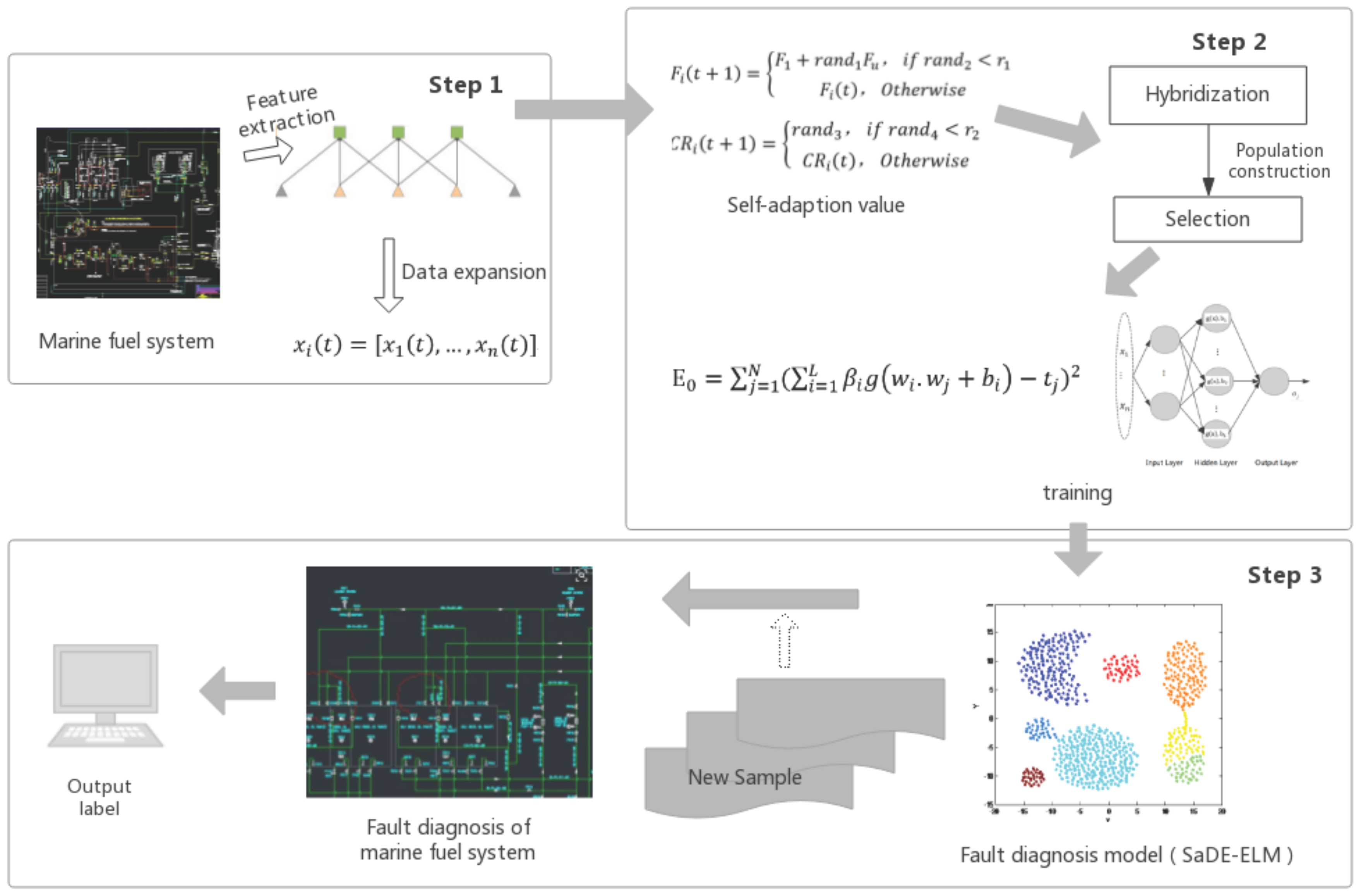
2. Research Framework

The system framework of the model proposed in this paper is shown in Figure 1 below. Its working principle is divided into three steps:
(1)
Extract the feature vectors of the state of the marine fuel system and use Gaussian white noise to expand the data samples;
(2)
A differential evolution algorithm is used to adaptively acquire the extreme learning initialization parameters, and the fault diagnosis model for marine fuel system is constructed for different types of data, and the minimum value of the objective function is estimated;
(3)
Get the test model with SaDE-ELM training and diagnose the most probable state of the marine fuel system according to the new sample.

3. Proposed Algorithm

The ELM algorithm belongs to one kind of single hidden layer feed-forward neural network. At present, there are BP neural networks that are commonly used single-layer neural network algorithms, but the main drawback of BP neural network lies in its training speed, which is not conducive to the acquisition of real-time information. However, ELM algorithm introduced in this paper can provide a model for the fault identification of marine fuel systems so as to get high-precision recognition results [7].
The common single hidden layer feedback neural network algorithm has the following problems in the practical application process [7].
(1)
The convergence of learning efficiency and algorithm is a positive relationship; that is, with the improvement of learning efficiency, the convergence of the algorithm is stronger, but when the learning efficiency is large enough, the stability of the algorithm will be worse, thus affecting the performance of the overall algorithm;
(2)
The algorithm is easy to fall into a local minimum, so when the algorithm finishes running, the operation ends at a distance far from the global minimum;
(3)
The training process of the algorithm can easily lead to the reduction of the overall generalization ability of the algorithm and thus affect the experimental accuracy of the algorithm;
(4)
The learning rules in the network are time-consuming and not conducive to the acquisition of real-time information.
Therefore, this paper first analyzes the content of the single hidden layer neural network algorithm before analyzing the extreme learning algorithm in detail, laying a good foundation for better studying the ELM algorithm [15]. According to the characteristics of a single-layer neural network, the overall construction process includes: input layer to hidden layer, and then to the output layer gradually propagate and regulate, but there is no relevant connection between the elements of the same layer, the only corresponding connection between different levels.

3.1. ELM Algorithm

In this section, we first introduce the principle of a single hidden-layer feed-forward neural network algorithm. After that, we describe the principle of ELM algorithm in details.
Figure 2 above is a single hidden layer neural network containing only one hidden layer.
Assuming there are N groups of samples ( x i , t i ) , so there are L hidden layer in x i = [ x i 1 , x i 2 , , x i n ] T n , t i = [ t i 1 , t i 2 , , t i n ] T ϵ   n . If g ( x ) is an activation function, the model is shown.
i = 1 L β i g i ( x j ) = i = 1 L β i g ( w i . x i + b i ) = o j ,   j = 1 ,   2 , , N
In the above formula, w i = [ w i 1 , w i 2 , , w i n ] T is the weight value between the hidden layer and the input layer. β 1 = [ β i 1 , β i 2 , , β i n ] T is the weight value between the hidden layer and the output layer. b i is the bias of the Zth hidden point.
The canonical model with L hidden layer points and g ( x ) can accurately approximate N data, expressing j = 1 L | o j t j | = 0 . According to β i , w i , and b i , we can get
i = 1 L β i g i ( w j . x j + b i ) = t j , j = 1 , 2 , , N
The above equations are summarized as
H β = T
Among
H ( w 1 , , w L , b 1 , , b n , x 1 , , x N ) = ( G ( w 1 , b 1 , x 1 ) G ( w L , b L , x L )     G ( w 1 , b 1 , x N ) G ( w L , b L , x N ) )
β = [ β 1 T β L T ] L × m , T = [ t 1 T t N T ] N × m
H is the corresponding output matrix of the hidden layer. The column of H is the output of the first hidden point. Generally speaking, in the process of training a hidden layer neural network, w ^ i , b ^ i ,   β ^ i ( i = 1 ,   ,   L ) need meet
| H ( w ^ 1 , , w ^ L , b ^ i , , b ^ L ) β ^ 1 b ^ i T | = H ( ( w ^ 1 , , w ^ L , b ^ i , , b ^ L ) β ^ 1 b ^ i T ) w i b i β i m i n
The equation above is equivalent to the equation below minimizing the following cost function.
E 0 = j = 1 N ( i = 1 L β i g ( w i . w j + b i ) t j ) 2
The solution of H is obtained by gradient descent learning algorithm for getting the minimum to | | H β T | | . The joint vector of ( w i , β i ) and ( b i ) is W . After finishing the iteration, we get the following formula:
W k = W k 1 η E ( W ) W
In the formula above, η is learning rate.
So, in view of the above single hidden-layer feed-forward neural network algorithm, it is easy to cause over-fitting in the actual operation process, the experimental real-time data acquisition rate being low and so on. Therefore, this type of method is called a problem that restricts the development of the neural network. The ELM algorithm is distinct from the neural network algorithm in the above sense. It sets different hidden layer numbers and obtains different analytical results for the output weights [16]. The ELM algorithm will be described and proved in detail as follows.
Figure 3 displays the structure of the ELM algorithm, including three levels: input, output layer, and hidden layer [17].
Assuming that the activation function g is infinitely different, so the number of hidden layers set by the ELM training is much smaller than that of the sample, namely L N . So, get the following theorem:
Theorem 3.
Assuming that there are N implicit nodes in the ELM corresponding to g : is infinitely different. N groups of samples ( x i , t i ) , x i ϵ n , t i ϵ m to n and in any interval and randomly determined w i and b i by any continuous probability distribution always meet H in ELM, which is reversible and also meet H | H β T | = 0 [18].
Proof. 
Assume vector c ( b i ) = [ g ( x i ) , , g ( x n ) ] T = [ g ( w i . x i + b i ) , , g ( w i . x n + b i ) ] T is that H is the ith column in Euclidean N − 1 space. b i ϵ ( a , b ) , ( a , b ) is in any interval of .
w i is obtained by continuous random distribution and randomly k k , if w i . x i w i . x k , c is the subset of N 1 dimension space, so vector α is orthogonal to the subspace.
( a ,   c ( b i ) c ( a ) ) = a 1 g ( b i + d 1 ) + a 2 g ( b i + d 2 ) + + a n g ( b i + d n ) z = 0
Among, d k = w i . x k , k = 1 , , n , z = α . c ( a ) , b i ϵ ( a , b ) , a n 0 , get:
g ( b i + d n ) = p r g ( b i + d p ) + z / α n
In the formula, γ p = α p α n , p = 1 , , n 1 . g ( x ) is infinitely different in any interval, so:
g ( l ) ( b i + d n ) = p r g ( l ) ( b i + d p ) , l = 1 ,   2 , , n , n + 1 ,
In the formula above, g ( l ) is the order guide of 1 of function g to b i . However, in the situation of N + 1 free coefficients r 1 , r 2 , , r n 1 , the linear equation is more than N 1 . There is a conflict between them. Therefore, subspace c does not belong to the smaller dimension N.
Therefore, there are certain probabilities in ( a , b ) , which can randomly select N hidden nodes corresponding to N bias values b 1 , , b n , and meet the corresponding c ( b 1 ) , , c ( b n ) can have a span to N . Showing that for all w i and b i , we can choose from all intervals of N and according to all successive probabilities, meeting that H is a full rank column vector.
Activation functions are Sigmoid, radial basis function, sine function, cosine function, exponential function, and non-regular function [19].
Unlike the common single-layer neural network parameters that need to be adjusted, Theorem 1 proves that w i and b i do not need to be adjusted empirically. After the initial parameters are set, coefficient matrix H of the ELM remains unchanged in the process of algorithm operation. So w i and b i , according to Equation (10), the solution process of single hidden layer neural network algorithm can be transformed into H β = T .
| H ( w 1 , ,   w n ^ , b 1 , , b n ^ ) β ^ T | = H ( w 1 , , w n ^ , b 1 , , b n ^ ) β ^ T β m i n
If there are hidden layer nodes L and samples N, with L = N . In the case where w i and b i are randomly obtained, H is a reversible square matrix and ELM can learn these samples with high precision.
But L is usually much smaller than N, and H is not a square. So, without the relations of w i , b i , β i ( i = 1 , , L ) meets H β = T . So the solution to linear equation above is
β ^ = H T
H + in the formula is the pseudo-inverse MP of H.
Theorem 2.
If the matrix G meets: G y is the least-squares solution of linear equation A x = y . In the situation of G = A + , A is the pseudo-inverse of M P [20,21,22,23].
Summarize the important properties of ELM algorithm according to Theorem 2:
(1) Especially, least-squares solution of x 0 = A + y and A x = y is:
| A x 0 y | = | A A + y y | = m i n A x y
(2) Then, all least-squares solutions of x 0 = A + y and A x = y have the smallest modulus:
| x 0 | = | A + y | | x | , x { x : | A x y | | A z y | , z n }
(3)  A x = y with the only smallest modulus and the least-squares solution is x = A + y x = A + y .
The Learning Rules of ELM: Known training samples = { x i , t i x i ϵ n } , t i ϵ R ,   i = 1 , , N , and transfer function g . L is the hidden layer node [24]:
(1) Get random hidden node parameters ( a i , b i ) , i = 1 , , L ;
(2) Getting of Hidden layer output matrix H;
(3) The calculation of output weight β : β = H + T .
H + is the pseudo-inverse MP of H. T = [ t 1 , , t N ] .
There are many calculation methods for the pseudo-inverse MP of H: the orthographic projection method, orthogonal method, iterative method, and singular value decomposition (SVD), etc. [25]. To reduce search and iteration in ELM algorithms, when H T H is non-singular, or the hogonal projection method is used with H 1 = ( H T H ) 1 H T . However, H T H cannot be known to be non-singular, and in some cases it is singular, so the orthogonal projection methods do not achieve the desired effect [26]. However, SVD is often used to obtain the MP pseudo-inverse method of H.
According to the research above, the following conclusions can be drawn:
(1) Training error term can reach the minimum. Especially, solving the least-squares solution of β ^ = H + T being H β = T , shows that this solution can be used to obtain the smallest error term:
| H β ^ T | = | H H + T T | = m i n | H β T |
In the actual operation of the algorithm, all the learning algorithms are aimed at obtaining the minimum error. However, the application process has limitations on the number of iterations, trapping into the local minimum, and other conditions, resulting in failure to obtain the desired effect, thereby reducing the performance of the algorithm.
(2) Minimum modulus of weight. All the solutions of β ^ = H + T and H β = T can find the minimal solution:
| β ^ | = | H + T | | β | , β ϵ { β : | H β T | | H z T | , Z ϵ N ¯ × N }
(3) The solution of H β = T has the uniqueness, β ^ = H + T .
In this paper, a new single-layer feed-forward neural network algorithm-extreme learning machine algorithm is introduced. After random estimation of the initial parameters is determined, the output values are analyzed and acquired. Any parameters in the ELM algorithm can be achieved by analysis instead of a simple iterative acquisition. Therefore, this paper also proves in theory that the ELM algorithm can guarantee the learning speed and has strong ability for generalization of the data. The ELM algorithm can be well applied, and the speed is improved by many times compared with the ordinary learning algorithm [18].
Compared with the commonly used BP neural network and SVM algorithm [27], the introduction of the ELM algorithm in this study has the following main advantages:
(1)
Ease of use. The model does not have to set a large number of parameters, and the training speed does not need to intervene and also can obtain better experimental results;
(2)
Fast learning. The learning time of the model is quite short, which is more conducive to the user’s real-time information acquisition;
(3)
Generalization performance is high, and the ELM algorithm has a better generalization performance for different data types;
(4)
Activation function selection is flexible. Alternative types of activation function in ELM algorithms are adequate.

3.2. The Differential Evolution (DE) Algorithm
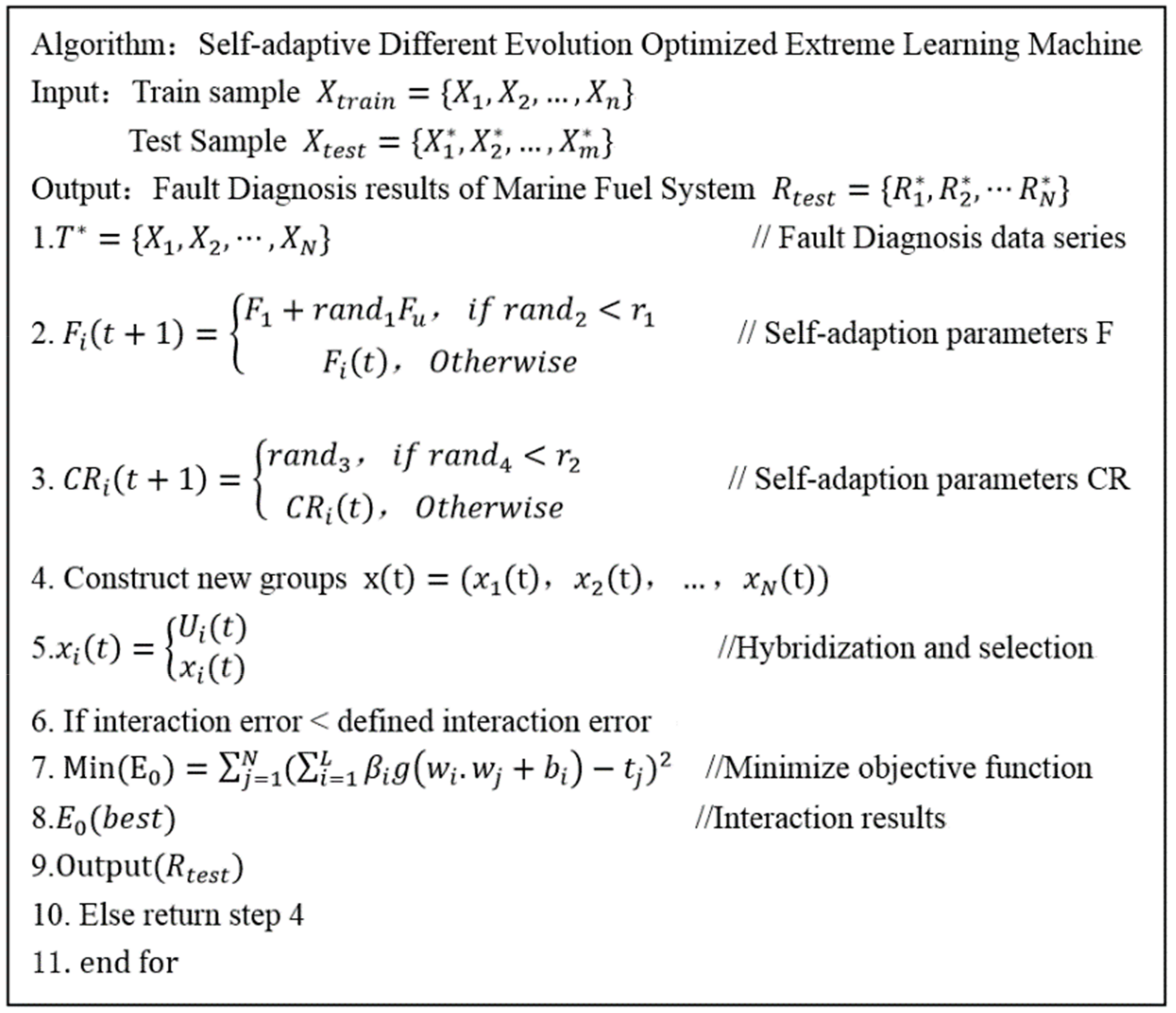
The differential evolution algorithm is a very effective algorithm for solving optimization problems [14]. DE is often used in conjunction with other algorithms to increase the efficiency of optimization algorithms for solving optimal problems [24]. The DE algorithm belongs to an evolutionary algorithm with high performance. In the process of solving the optimization problem, it has the characteristics of fast convergence. The central idea of the algorithm includes the following three steps [28,29,30,31,32]:
(1) Variation
Individuals are treated using the following formula to obtain variant individuals.
V i = X i 1 + F ( X i 2 X i 3 )
In the formula above, V i represents the mutated individual. X i represents the ith individual in the groups. Among them, i , i 1 , i 2 , i 3 { 1 , 2 , , N p } ,     N p is group size and N p 4 , F [ 0   2 ] is control parameters to have a regulation to ( X i 2 X i 3 ) .
(2) Hybridization
The hybridization process is the reorganization of the old individual X i and the new individual V i , generating new members U i .
U i j = { U i j ,   i f   r a n d j ( 0 , 1 ) C R j = k   X i j ,   O t h e r w i s e
CR is the main parameter in the DE algorithm, indicating the hybrid probability; In k ϵ { 1 , 2 , , D } , D is the spatial dimension of the problem search.
(3) Selection
Selecting individuals suitable for group’s development between old individuals and new individuals,
X i = { U i ,   i f   f ( U i ) f ( X i ) X i ,   O t h e r w i s e

3.3. SaDE-ELM

Since the ELM algorithm generates initialization parameters randomly, the initialization result has a significant impact on the output weight matrix. Therefore, In order to improve the efficiency of the ELM algorithm, based on the initialization results, a DE algorithm is introduced to solve the initial parameters of the ELM. However, there are unknown parameters that need to be initialized in the DE algorithm. If the artificial setting is based on experience, the result is subjective and the automatic diagnosis of the fault data cannot be achieved. So, in this study, we propose a SaDE-ELM algorithm, and optimize the DE algorithm to achieve the adaptive acquisition of unknown parameters of the DE algorithm, thereby improving the accuracy of fault diagnosis of SaDE-ELM. The flowchart is shown in Figure 4 below.
The main ideas of the SaDE-ELM algorithm are as follows:
(1)
The main parameters of SaDE-ELM: Scale factor F and hybrid probability CR. The parameters F and CR have a great influence on the convergence, stability and convergence speed of the DE algorithm. SaDE-ELM is proposed. The adjustment process of parameters F and CR is as follows:
F i ( t + 1 ) = { F 1 + r a n d 1 F u ,   i f   r a n d 2 < r 1 F i ( t ) ,   O t h e r w i s e
C R i ( t + 1 ) = { r a n d 3 ,   i f   r a n d 4 < r 2 C R i ( t ) ,   O t h e r w i s e
F i ( t + 1 ) is the adaptive acquisition scaling factor. C R i ( t + 1 ) is the adaptive acquisition of hybrid probability and is an evenly distributed random number within the interval [ 0   1 ] ; r a n d j ,   j { 1 , 2 , 3 , 4 } are evenly distributed random numbers within the interval [ 0   1 ] . F 1 = 0.1 ; F u = 0.9 ,     r 1 , r 2 are adjustment parameters.
(2)
Construct groups. Based on adaptive acquisition parameters, construct new groups x ( t ) = ( x 1 ( t ) , x 2 ( t ) , , x N ( t ) ) . Each sample is the state of feature matrix m × d of the marine fuel system, namely m × d = D .
(3)
Individuals of the groups are crossed and selected. The final choice of highly competitive individuals is as follows:
x i ( t ) = { U i ( t ) ,   i f   E 0 ( U i ( t ) ) E 0 ( x i ( t ) ) x i ( t ) ,   O t h e r w i s e
E 0 ( · ) represents the minimum value E 0 in the objective function, namely the objective function value of each individual in groups.
(4)
Define iteration errors. According to the defined number of iterations to determine whether the iteration is terminated, if you continue to step (2) within the iteration range, otherwise go to the next step.
(5)
Output the best iteration result, E 0 ( b e s t ) and corresponding hidden layer weight β ^ .
(6)
Output ELM algorithm of fault diagnosis results for a marine system.
The pseudocode is as following Figure 5.

4. Model Construction and Simulation Experiment Results

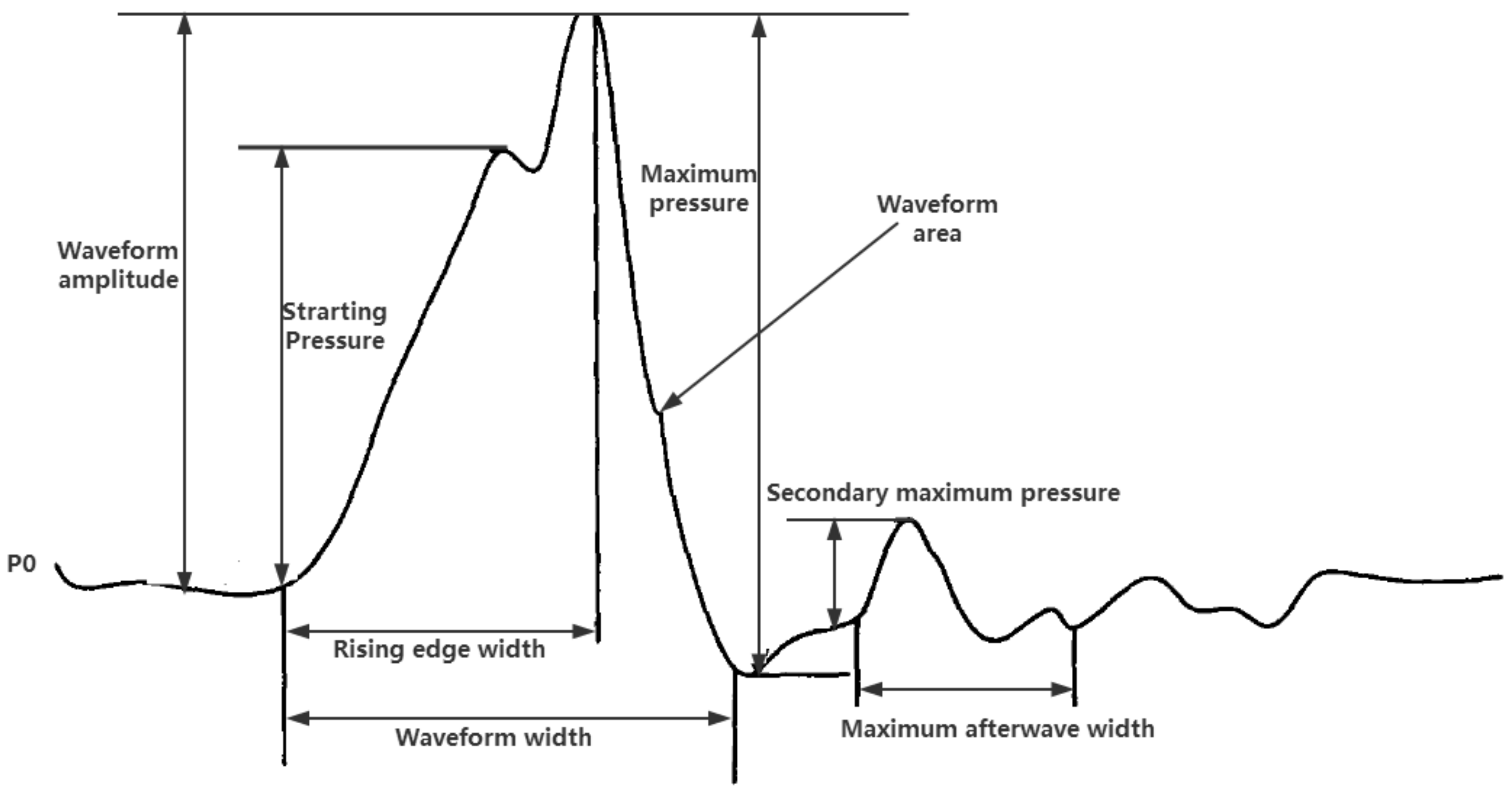
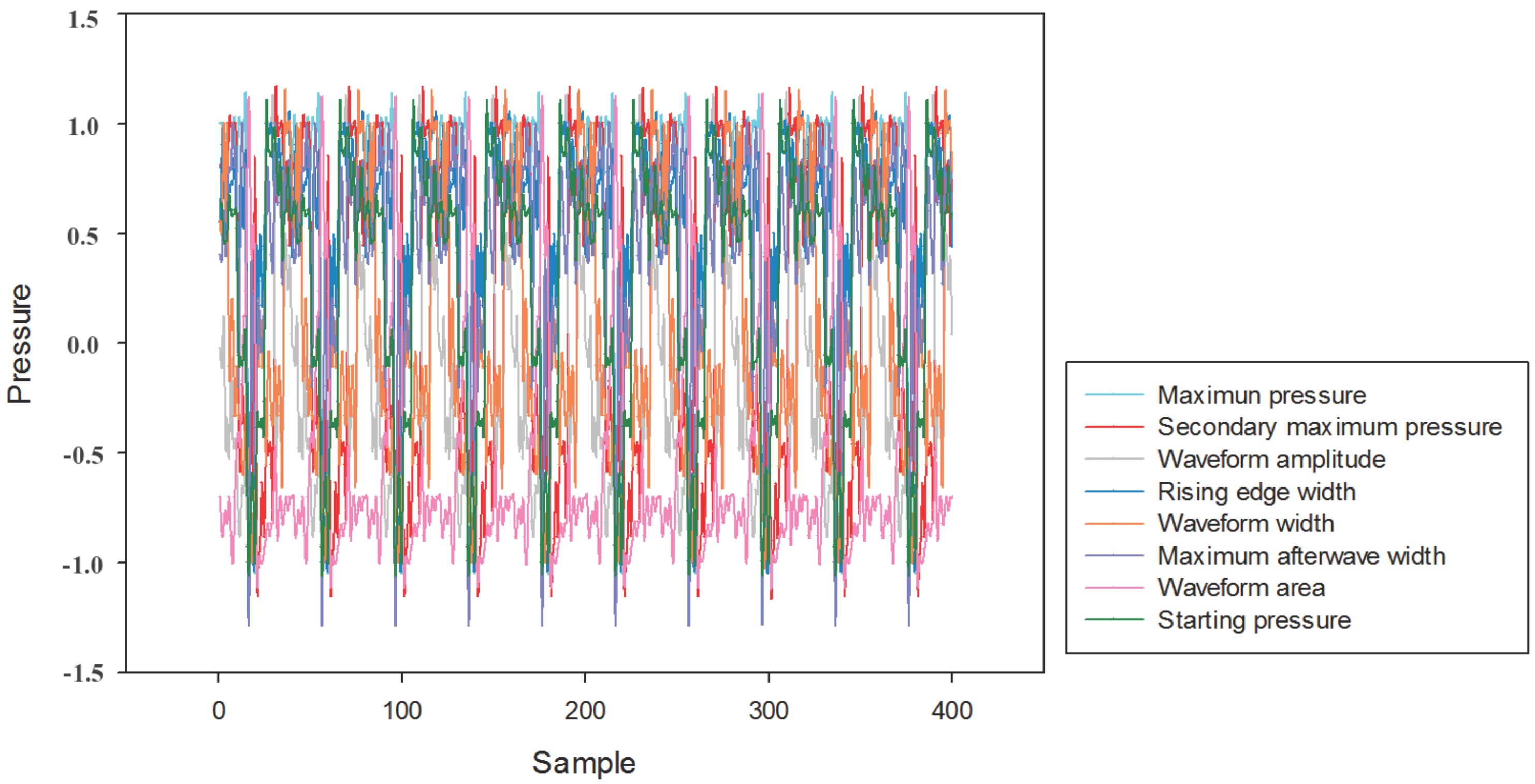
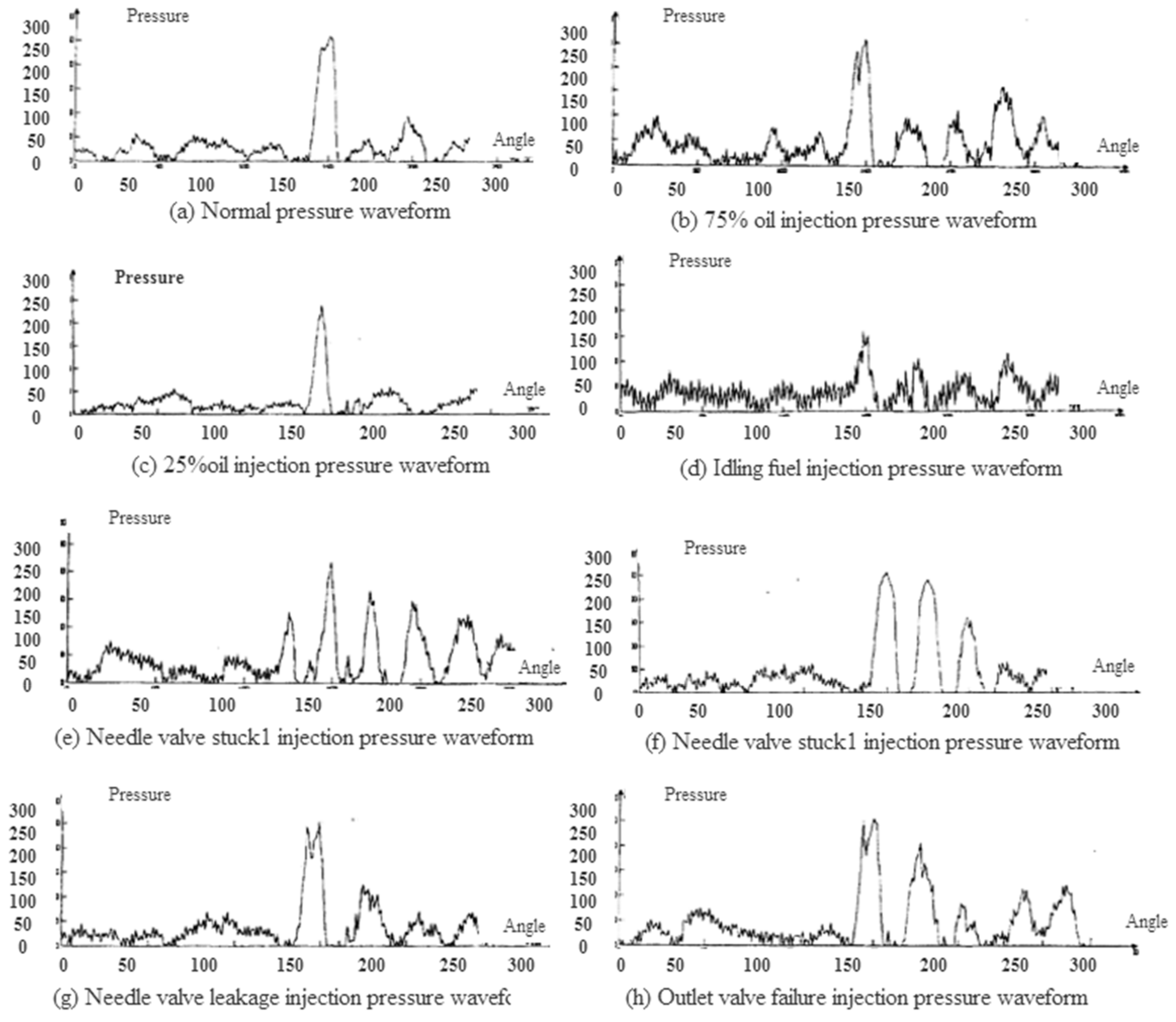
4.1. Extraction of Fault Feature for Marine Fuel System

We collect data from the measurement data of “fuel injection atomization test rig”. The main reason for choosing the data include two points: (1) the status data of the marine fuel system is obtained by simulating the operational status of the marine fuel system under realistic scenarios. The fuel injection atomization test bench is designed and built according to the actual fuel supply injection system and is consistent with the working state of the marine fuel system in the real situation. (2) The fault data obtained to cover the possible types of faults of the marine fuel system more comprehensively. Therefore, it is believed that the data used in this paper has a certain representation in the process of marine fuel system fault identification experiment and can be close to the real situation data, providing theoretical support for the fault identification work in the real task of the marine fuel system.
Figure 6 is the illustration of the marine fuel system.
The marine fuel system is divided into two parts: the low-pressure oil line and the high-pressure oil line. The low-pressure oil line includes the fuel tank, the circulating pump, the fuel filter, and the low-pressure oil pipe. The high-pressure oil line mainly includes the injection pump, the injector, and the high-pressure oil pipe. The basic task of the marine fuel system is mainly accomplished by the high-pressure oil circuit, which is a key part of the oil supply system. The state information of the marine fuel system is mainly reflected in the pressure waveform of the high pressure fuel pipe. When a fault occurs somewhere, the original fuel supply state will change, and the pressure and tassel parameters of the fuel flow will change accordingly. The pressure waveform causes changes in the waveform shape and waveform parameter values. Therefore, this paper selects the pressure wave characteristics of the high-pressure pipe for fault analysis. In order to obtain better diagnostic results, the paper is based on literature research [33] and selects commonly used pressure wave feature as shown in the following Figure 7, including eight parameters of the maximum fuel injection pressure, injector valve opening pressure, sub-maximum pressure, waveform amplitude, rising edge width, waveform width, maximum residual width, waveform area.

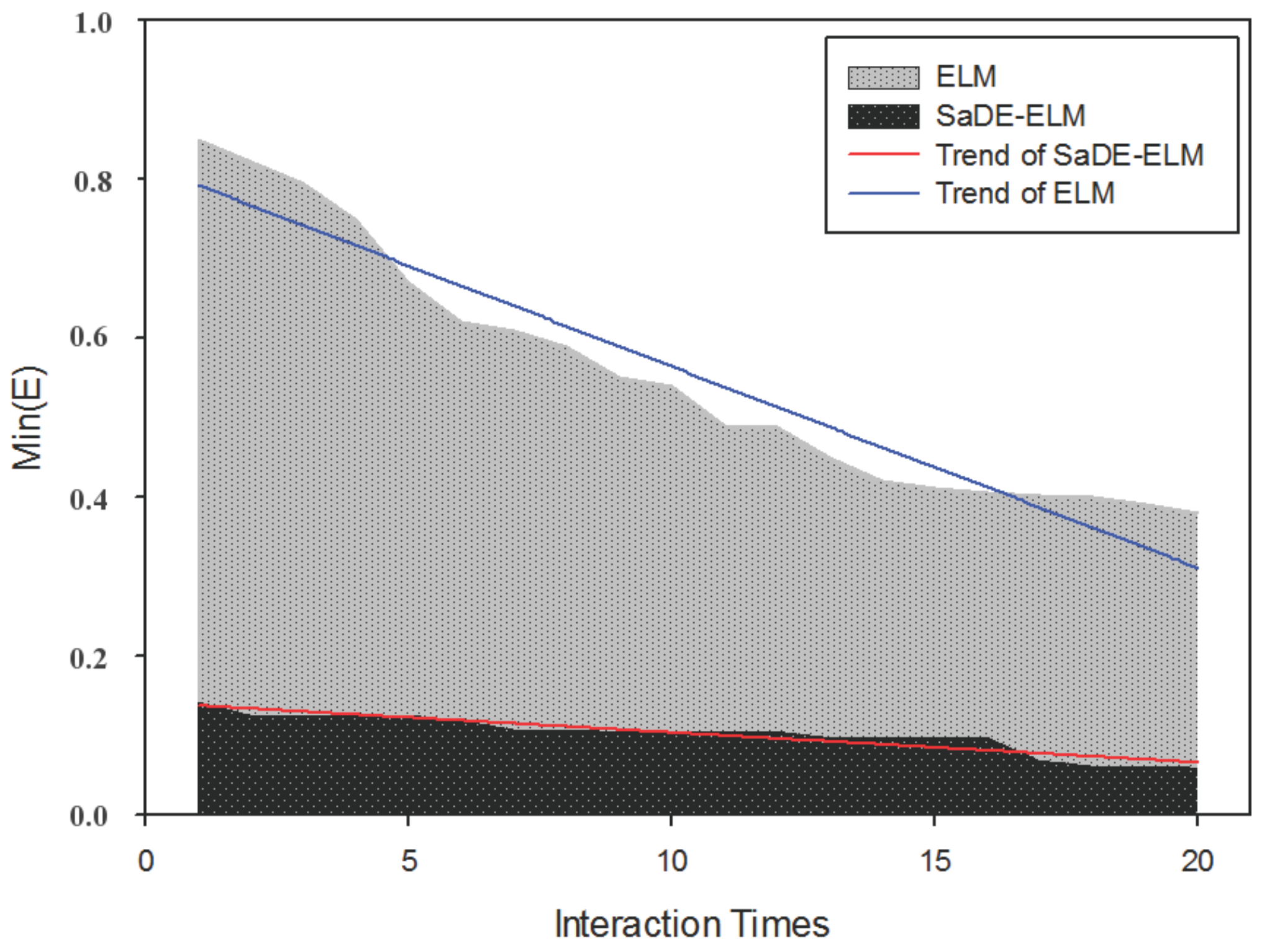
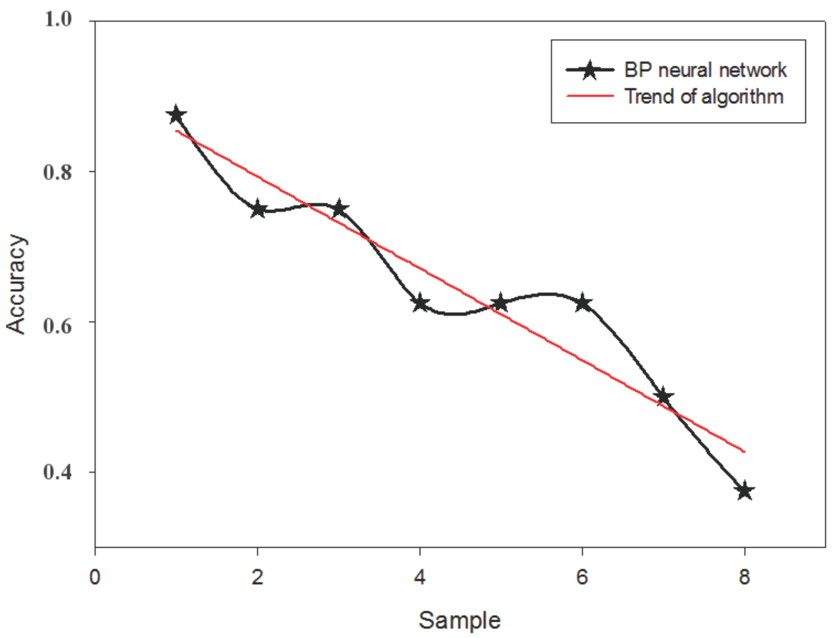
4.2. Model Construction

In order to increase the number of training samples and make the established GMM more representative, add the characteristic values above to Gaussian white noise of 40 dB, 45 dB, 50 dB, 55 dB, 60 dB, 65 dB, 70 dB, 75 dB, and 80 dB. The preliminary data are expanded to 400 groups. The 400 sets of data are used as training samples to construct a training model for SaDE-ELM. Then, on the basis of the training model, test samples are input to determine the situation of the proposed method of fault diagnosis for marine fuel systems.
The descriptive analysis of the pressure wave characteristics of the initial 400 sets of data used in the research is shown in Figure 8 below.
One of the common faults of the fuel system is the poor quality fuel when the ship is refilling, which has caused some problems in the fuel system. According to the combination of different pressure waveform characteristics, the following types of marine fuel system states are formed: normal state, insufficient fuel supply (75% oil, 25% oil, idle oil volume), stuck needles to plug holes (small oil quantity, standard oil quantity), needle valve leakage, and oil valve failure. That is, eight sub-states, normal injection, 75% oil volume, 25% oil volume, idle oil volume, injector needle stuck 1, injector needle stuck 2, injector needle leakage, and high-pressure pump outlet valve failure [33]. Where the system state except the normal state belongs to the type of faults of the marine fuel system. In the condition of insufficient oil supply, the waveform will decrease with the decrease of oil supply, the waveform area will decrease, and the average waveform will also decrease. When the needle valve is located in faults, the pressure wave rises very quickly and the pressure wave curve is sharp. And the reflected wave is quite intense in the pipe, the durable time is longer, and the residual pressure is higher than the normal pressure. Compared the standard oil volume with the small oil volume, the amount of oil and residual pressure is greater, and the attenuation is faster. The leakage of the needle valve will cause the fuel pressure to drop; when the outlet valve fails, the residual pressure of the fuel is high, the pressure fluctuation is obvious, and the attenuation is slow.
Figure 9 below shows the pressure waveforms of different states of the marine fuel system.
In the process of constructing a model through SaDE-ELM, the objective function E 0 gradually iterates to obtain the minimum value. First, judge the effect of different hidden layer numbers on the fault diagnosis of EL algorithm and SaDE-ELM algorithm and select 20 times of the default number of iterations, as shown in Table 1.
The experimental results show that, with the increase of the number of hidden layers, the error of the algorithm gradually decreases, but the time cost of the training model increases slightly. The SaDE-ELM algorithm has a better performance for the fault diagnosis of marine fuel systems. All test samples can be classified into the correct state types, while the ELM algorithm also increases with the number of hidden layers. The training and testing errors gradually decrease, but the fault diagnosis effect is worse than the SaDE-ELM algorithm. SaDE-ELM is 25 in hidden layers, and the training error is 0, so the subsequent comparison experiment chooses 25 hidden layers to construct the fault diagnosis model of the marine fuel system.
In order to investigate the convergence of the objective function of the extreme learning algorithm and SaDE-ELM to the state recognition process of the marine fuel system, the proposed method is suitable for the fault diagnosis of the marine fuel system. The convergence process can be observed in Figure 10. With the increase of the number of iterations, the ELM algorithm quickly decreases the value of the objective function. However, due to the low precision of the algorithm, the final converged objective function value is close to 0.3, which is still relatively large. In this paper, SaDE-ELM is proposed. The value of the objective function at the initial point is less than 0.2. As the number of iterations increases, the ultimate objective function gradually approaches 0, achieving a better target function minimization effect. At the same time, as the number of iterations continues to increase, the objective function value tends to be stable, close to 0.
Based on the experimental results above, the commonly used algorithms for fault diagnosis of marine fuel systems, BP (Back Propagation) neural network, and SVM (support vector machine) algorithm are selected to compare and analyze the experimental results, including the accuracy of fault diagnosis and the time of fault diagnosis. As shown in Table 2.
Comparing the experimental results in Table 2, it is found that SaDE-ELM has a higher recognition rate for the faults of the marine fuel system than the commonly used algorithm BP neural network and the SVM, and SaDE-ELM is not significantly higher than that of the BP neural network algorithm and the SVM, and the correct rate is obviously higher than other commonly used algorithms.
To further demonstrate the recognition status of different fault diagnosis algorithms for 8 types of samples, as shown in Figure 11, Figure 12, Figure 13 and Figure 14.
From Figure 11 to Figure 14, it can be seen that the fault diagnosis method of marine fuel system based on SaDE-ELM proposed in this paper can correctly identify each type of fault, and other three algorithms are certain error rate for the identification of eight types of samples, especially for the fourth type of sample—idle oil identification poor effect, and there have been errors. The reason is perhaps that the characteristics of this kind of sample are close to those of the type 3 sample, so the conventional fault diagnosis algorithm cannot be discriminated. The SaDE-ELM proposed in this paper can better identify the fuzzy faults of this kind of data features.
The BP neural network algorithm also belongs to a single hidden layer feed-forward neural network algorithm. The weight of the algorithm is utilized to judge the experimental accuracy of the entire algorithm [25]. However, its diagnostic effect on the faults of the marine fuel system is far worse than that of SaDE-ELM. The BP neural network algorithm and the conventional single hidden layer feedback neural network algorithm in the actual application process algorithm is easy to fall into a local minimum, resulting in the poor generalization of the algorithm.
Combining the DE algorithm with ELM algorithm solves the limitations above of the single hidden layer feedback neural network algorithm. At the same time, it obtains the parameters of the DE algorithm through an adaptive approach and also addresses the problem that the algorithm itself sets rely on empirical parameters. Therefore, it is illustrated that the method proposed in this paper can better solve the limitations of the existing research lacking the high accuracy of fault diagnosis method for the marine fuel system, and also solve the problem of the low initialization precision of the ELM algorithm and improve the accuracy of the algorithm. The accuracy of the SVM algorithm of fault diagnosis for marine fuel system is worse than the method proposed in this paper because the SVM algorithm is more difficult to construct the hyperplane to distinguish different types of faults in the face of more types of faults. So the accuracy is lower.

5. Conclusions

In view of the low accuracy of the existing fault diagnosis methods for marine fuel systems, this paper proposes a fault diagnosis method for marine fuel system based on SaDE-ELM and extracts feature vector of eight dimensions depending on the characteristics of the marine fuel system. When constructing an ELM model, the DE algorithm is first used to self adaptively solve its initialization problem to construct a complete and efficient fault diagnosis model. The experimental results revealed that the proposed method of fault diagnosis for marine fuel system based on the SaDE-ELM algorithm can achieve a diagnostic accuracy of 100%. It is superior to the traditional BP neural network algorithm and SVM algorithm. Moreover, it can be ruled out that manually setting parameters has a certain guiding effect on the results, which is an efficient fault diagnosis method and has great practical value and also provides a new method for the problem of fault diagnosis for the marine fuel system.
In practice, we will judge the real-time status of the system to realize the fault diagnosis of the marine fuel system. The real-time waveform feature data and fault diagnosis model are combined. As the fuel injection atomization test bench is designed and built according to the actual fuel supply injection system, the collected data has a strong similarity with the actual situation. Meanwhile, the data comprehensively covers the possible faults of the marine fuel system. We therefore believe that the choice of experimental data is reasonable and representative of actual data and that the proposed methodology can effectively be used for fault diagnosis of marine fuel systems in actual.

Author Contributions

Y.W. conceived and designed the experiments, Y.Y. performed the experiments, and Y.W. analyzed the data and wrote the paper.

Acknowledgments

This work is financially supported by the National Natural Science Foundation of China (No. 51479018) and the Fundamental Research Funds for the Central University (No. 3132013337).

Conflicts of Interest

The authors declare no conflict of interest.

References

  1. Han, L. Intelligent Fault Diagnosis Technology of Diesel Engine; National Defense Industry Press: Beijing, China, 2005. [Google Scholar]
  2. Liu, Y.; Zhang, J.; Qin, K.; Xu, Y. Diesel engine fault diagnosis using intrinsic time-scale decomposition and multistage Adaboost relevance vector machine. Proc. Inst. Mech. Eng. Part C 2018, 232, 881–894. [Google Scholar] [CrossRef]
  3. Govindaraj, T.; Su, Y.L.D. A model of fault diagnosis performance of expert marine engineers. Int. J. Man-Mach. Stud. 1988, 29, 1–20. [Google Scholar] [CrossRef]
  4. Autar, R.K. An automated diagnostic expert system for diesel engines. J. Eng. Gas Turbines Power 1996, 118, 673–679. [Google Scholar] [CrossRef]
  5. Cai, C.; Weng, X.; Zhang, C. A novel approach for marine diesel engine fault diagnosis. Clust. Comput. 2017, 20, 1691–1702. [Google Scholar] [CrossRef]
  6. Jiang, W.; Hu, W.; Xie, C. A new engine fault diagnosis method based on multi-sensor data fusion. Appl. Sci. 2017, 7, 280. [Google Scholar] [CrossRef]
  7. Huang, G.B.; Zhou, H.; Ding, X.; Zhang, R. Extreme learning machine for regression and multiclass classification. IEEE Trans. Syst. Man. Cybern. B Cybern. 2012, 42, 513–529. [Google Scholar] [CrossRef] [PubMed]
  8. Jin, C.; Zhao, W.; Liu, Z.; Lee, J.; He, X. A vibration-based approach for diesel engine fault diagnosis. In Proceedings of the 2014 IEEE Conference on Prognostics and Health Management (PHM), Cheney, WA, USA, 22–25 June 2014; pp. 1–9. [Google Scholar]
  9. Widodo, A.; Yang, B.S. Support vector machine in machine condition monitoring and fault diagnosis. Mech. Syst. Signal Process. 2007, 21, 2560–2574. [Google Scholar] [CrossRef]
  10. Zhang, X.L.; Xu, Y.J. Fault Diagnosis for Diesel Engine Cylinder Head Based on Genetic-SVM Classifier. In Applied Mechanics and Materials; Trans Tech Publications: Zürich, Switzerland, 2014; Volume 590, pp. 390–393. [Google Scholar]
  11. Wang, Y.M.; Cui, T.; Zhang, F.J.; Dong, T.; Li, S. Fault diagnosis of diesel engine lubrication system based on PSO-SVM and centroid location algorithm. In Proceedings of the 2016 International Conference on Control, Automation and Information Sciences (ICCAIS), Ansan, Korea, 27–29 October 2016; pp. 221–226. [Google Scholar]
  12. Zhang, Z.; Guo, H. Research on Fault Diagnosis of Diesel Engine Based on PSO-SVM. In Proceedings of the 6th International Asia Conference on Industrial Engineering and Management Innovation, Tianjin, China, 25–26 July 2015; Atlantis Press: Paris, France, 2016; pp. 509–517. [Google Scholar]
  13. Blanke, M.; Kinnaert, M.; Lunze, J.; Staroswiecki, M.; Schröder, J. Diagnosis and Fault-Tolerant Control; Springer: Berlin, Germany, 2006. [Google Scholar]
  14. Padma, K.; Vaisakh, K. Oposition-based modified differential evolution algorithm with SSVR device under different load conditions. In Proceedings of the IEEE Power, Communication and Information Technology Conference, Bhubaneswar, India, 15–17 October 2015; pp. 935–940. [Google Scholar]
  15. Li, Y.; Guo, P.; Li, X. Short-Term Load Forecasting Based on the Analysis of User Electricity Behavior. Algorithms 2016, 9, 80. [Google Scholar] [CrossRef]
  16. Tang, J.; Deng, C.; Huang, G.B. Extreme Learning Machine for Multilayer Perceptron. IEEE Trans. Neural Netw. Learn. Syst. 2017, 27, 809–821. [Google Scholar] [CrossRef] [PubMed]
  17. Liu, X.; Lin, S.; Fang, J.; Xu, Z. Is extreme learning machine feasible? A theoretical assessment (part I). IEEE Trans. Neural Netw. Learn. Syst. 2017, 26, 7–20. [Google Scholar] [CrossRef] [PubMed]
  18. Zhang, L.; Zhang, D. Evolutionary Cost-Sensitive Extreme Learning Machine. IEEE Trans. Neural Netw. Learn. Syst. 2017, 28, 3045–3060. [Google Scholar] [CrossRef] [PubMed] [Green Version]
  19. Yu, L.; Dai, W.; Tang, L. A novel decomposition ensemble model with extended extreme learning machine for crude oil price forecasting. Eng. Appl. Artif. Intell. 2016, 47, 110–121. [Google Scholar] [CrossRef]
  20. Li, S.; You, Z.H.; Guo, H.; Luo, X.; Zhao, Z.Q. Inverse-Free Extreme Learning Machine with Optimal Information Updating. IEEE Trans. Cybern. 2016, 46, 1229. [Google Scholar] [CrossRef] [PubMed]
  21. Teo, T.T.; Logenthiran, T.; Woo, W.L. Forecasting of photovoltaic power using extreme learning machine. In Proceedings of the IEEE Innovative Smart Grid Technologies—Asia, Bangkok, Thailand, 3–6 November 2015; pp. 1–6. [Google Scholar]
  22. Sajjadi, S.; Shamshirband, S.; Alizamir, M.; Yee, L.; Mansor, Z.; Manaf, A.A.; Mostafaeipour, A. Extreme learning machine for prediction of heat load in district heating systems. Energy Build. 2016, 122, 222–227. [Google Scholar] [CrossRef]
  23. Sivalingam, K.C.; Mahendran, S.; Natarajan, S. Forecasting Gold Prices Based on Extreme Learning Machine. Int. J. Comput. Commun. Control 2016, 11, 372. [Google Scholar] [CrossRef]
  24. Liu, Z.X.; Zhen-Yu, L.U.; Huang, P.F. Parameter Identification of Space Robot Based on Recursive Different Evolution Algorithm. J. Astronaut. 2014, 35, 1127–1134. [Google Scholar]
  25. Naji, S.; Keivani, A.; Shamshirband, S.; Alengaram, U.J.; Jumaat, M.Z.; Mansor, Z.; Lee, M. Estimating building energy consumption using extreme learning machine method. Energy 2016, 97, 506–516. [Google Scholar] [CrossRef]
  26. Al-Yaseen, W.L.; Othman, Z.A.; Nazri, M.Z.A. Multi-level hybrid support vector machine and extreme learning machine based on modified K-means for intrusion detection system. Expert Syst. Appl. 2017, 67, 296–303. [Google Scholar] [CrossRef]
  27. Zhong, H.; Miao, C.; Shen, Z.; Feng, Y. Comparing the learning effectiveness of BP, ELM, I-ELM, and SVM for corporate credit ratings. Neurocomputing 2014, 128, 285–295. [Google Scholar] [CrossRef]
  28. Liu, Y. Research Progress on Different Evolution Algorithm. Sci. Mosaic 2013, 3, 004. [Google Scholar]
  29. Lu, Q.; Zhang, X.; Wen, S.; Lan, C. Comparison Four Different Probability Sampling Methods based on Differential Evolution Algorithm. J. Adv. Inf. Technol. 2012, 3, 206–214. [Google Scholar] [CrossRef]
  30. Fu-Heng, Q.U.; Ya-Ting, H.U.; Yang, Y.; Sun, S.Z.; Yuan, L.H. Differential evolution algorithm with different strategies and control parameters. J. Comput. Appl. 2011, 31, 3097–3100. [Google Scholar]
  31. Lin, J.L.; Tsai, Y.H.; Yu, C.Y.; Li, M.S. Interaction Enhanced Imperialist Competitive Algorithms. Algorithms 2012, 5, 433–448. [Google Scholar] [CrossRef] [Green Version]
  32. Qin, A.K.; Huang, V.L.; Suganthan, P.N. Differential Evolution Algorithm with Strategy Adaptation for Global Numerical Optimization. IEEE Trans. Evol. Comput. 2009, 13, 398–417. [Google Scholar] [CrossRef]
  33. Corallo, A.; Margherita, A.; Pascali, G. Digital Mock-up to Optimize the Assembly of a Ship Fuel System. J. Model. Simul. Syst. 2010, 1, 4–12. [Google Scholar]
Figure 1. Research framework.
Algorithms 11 00082 g001
Figure 2. Single hidden layer neural network framework.
Algorithms 11 00082 g002
Figure 3. Structure of Extreme Learning Machine (ELM) algorithm.
Algorithms 11 00082 g003
Figure 4. Flow chart of the Self-adaptive Different Evolution Optimized Extreme Learning Machine (SaDE-ELM) algorithm.
Algorithms 11 00082 g004
Figure 5. Pseudocode of the proposed SaDE-ELM algorithm.
Algorithms 11 00082 g005
Figure 6. Marine fuel oil system. 1—tank, 2—strainer, 3—circulating pump, 4—delivery valve, 5—fuel system filter, 6—high pressure pump, 7—high-pressure pipe, 8—injector, and 9—return pipe.
Algorithms 11 00082 g006
Figure 7. Pressure waveform characteristic parameters.
Algorithms 11 00082 g007
Figure 8. Pressure wave characteristics of training data.
Algorithms 11 00082 g008
Figure 9. Pressure waveforms for the different states of the marine fuel system.
Algorithms 11 00082 g009
Figure 10. Comparison of the convergence effect of the algorithm.
Algorithms 11 00082 g010
Figure 11. BP neural network algorithm for marine fuel system fault diagnosis.
Algorithms 11 00082 g011
Figure 12. Support vector machine algorithm for marine fuel system fault diagnosis.
Algorithms 11 00082 g012
Figure 13. Extreme learning machine algorithm for marine fuel system fault diagnosis.
Algorithms 11 00082 g013
Figure 14. SaDE-ELM algorithm for marine fuel system fault diagnosis.
Algorithms 11 00082 g014
Table 1. Quantity of hidden layer impacts on the algorithm.
Hidden Layer NumberTraining TimeTraining ErrorTest Error
ELMSaDE-ELMELMSaDE-ELMELMSaDE-ELM
10.1213.7910.8750.811
51.3426.5220.2750.1250.2750
102.52711.3570.1250.10.1250
153.71211.3880.0750.050.0750
203.85518.7670.0650.050.0650
254.52119.0320.02500.0250
Table 2. Performance comparison of different algorithms for fault diagnosis of the marine fuel system.
AlgorithmTraining TimeTraining ErrorTest Error
BP neural network12.5310.50.625
SVM10.0120.250.25
SaDE-ELM19.03200

