Distributed Combinatorial Maps for Parallel Mesh Processing


1
CNRS, LIRIS, UMR5205, Université de Lyon, 69622 Lyon, France
2
Faculté des Sciences et Technologies Department, Université Lyon 1, 69100 Lyon, France
*
Author to whom correspondence should be addressed.
Algorithms 2018, 11(7), 105; https://doi.org/10.3390/a11070105
Submission received: 31 May 2018
/
Revised: 9 July 2018
/
Accepted: 9 July 2018
/
Published: 13 July 2018
(This article belongs to the Special Issue Efficient Data Structures)
Abstract
:We propose a new strategy for the parallelization of mesh processing algorithms. Our main contribution is the definition of distributed combinatorial maps (called n-dmaps), which allow us to represent the topology of big meshes by splitting them into independent parts. Our mathematical definition ensures the global consistency of the meshes at their interfaces. Thus, an n-dmap can be used to represent a mesh, to traverse it, or to modify it by using different mesh processing algorithms. Moreover, an nD mesh with a huge number of elements can be considered, which is not possible with a sequential approach and a regular data structure. We illustrate the interest of our solution by presenting a parallel adaptive subdivision method of a 3D hexahedral mesh, implemented in a distributed version. We report space and time performance results that show the interest of our approach for parallel processing of huge meshes.
1. Introduction
Meshes are an essential concept for representing objects in computers. They are used for example in Computer-Aided Design, in geometric modeling, or in physical simulations with the Finite Element Method. Many data structures have been defined to describe meshes. They can be separated into two main categories: (1) constructive solid geometry (CSG), where objects are described as collections of basic primitives, combined together by Boolean operations; (2) boundary representation models (B-rep), where the boundaries of objects are described by a description of the surface elements (vertices, edges, faces) connected together by boundary relations. B-rep models are usually more flexible than CSG ones and have richer operations. These advantages explain why B-rep models are very often used in applications that want to describe and modify objects.
The objects handled are often polygon meshes, described only by their surfaces. Indeed, this type of description is enough in many applications, as for example in the main 3D computer graphics applications where we only want to visualize, analyze and modify the shape of objects [1]. However, this type of model cannot be used in applications that need to represent both the exterior and the interior volumes of a 3D object [2]. This is the case for simulation applications, which require to represent the interior volumes of an object to associate material properties and perform computations for each internal element [3]. This is also the case in modeling applications of buildings that describe a building as an assembly of several 3D objects [4]. These applications require volume meshes to represent and to handle both the exterior and the interior of 3D objects. Lastly, some applications require to describe objects in higher dimension. We can cite for example some problems in visibility and in geometric optimization that involve generalized Voronoi diagrams in any dimension [5], or some work that would like to represent 3D objects added with some feature dimension spaces, such as for example the project of urban modeling in higher dimensions [6], or the reconstruction of 5D respiratory motion models [7].
These different needs show the interest of having a generic data structure that is able to describe meshes in any dimension.
Many different data structures were defined to represent polygon meshes. A first model defined was the winged-edge data structure [8], followed by many solutions based on a similar idea, each provides different advantages, drawbacks and power of representation. We can cite the half-edges or DCEL [9,10,11], quad-edges [12], radial-edges [13], corner table [14], etc. Other works in the field of combinatorics defined solutions in order to represent planar graphs embedded in the plane, or polyhedral surfaces, such as [15,16,17,18]. However, all these data structures are only able to describe surface meshes: it is not possible to describe subdivided 3D objects made of several combinations of atomic elements, nor to describe objects in higher dimension.
Few data structures were defined to represent volumetric meshes, like for example facet-edge [19], handle-face [20], OpenVolumeMesh [21] or AHF [22]. However, these solutions are not able to describe nD meshes. The choice of a data structure becomes very limited when we want to represent nD objects. Several graph-based solutions were proposed. For example, in the incidence graph [23,24], each cell is represented as a node, and an arc exists between each pair of nodes corresponding to two incident cells whose dimensions differ by one. This data structure is simple, but has several drawbacks. First, it cannot represent multi-incidence relations, which often occur in real applications. Second, the incidence graph is not ordered, e.g., it does not allow us to iterate through all the vertices of a face in a given order, which leads to complex and inefficient operations.
In order to solve these drawbacks, combinatorial maps [25,26] were defined. This model has several advantages that justify its use. (1) There is a formal mathematical definition, including consistency constraints, with a clear distinction between the structure information and the shape information; (2) This mathematical foundation allows us to formally define the sets of corresponding subdivisions; this is important, since many classical mathematical notions and properties can thus be applied to combinatorial maps; (3) Since the structure is well-defined, the operations producing combinatorial maps are also well-defined, i.e., they construct the representation of valid geometric objects; (4) Elementary local operations can be conceived, and make it possible to carefully control the objects during their construction; (5) Many operations exist, often based on the elementary local operations, to compute characteristics and to modify nD meshes; (6) Efficient data structures have been conceived, based on combinatorial maps, together with operations for handling these structures; (7) The formal links between combinatorial maps and ordered models, combinatorial maps and incidence graphs, combinatorial maps and simplicial structures, are well-known; it is thus possible to conceive conversion operations between all these structures; (8) Lastly, a free implementation is proposed, including several operations, in Cgal [27], a major C++ library of computational geometry.
To sum up, this topological representation can be used to describe an nD mesh, while providing high level operations to iterate through the cells of the mesh, retrieve the incidence and adjacency relations between the cells, and modify the mesh by using the numerous existing operations. For all these reasons, combinatorial maps were used in many applications (see references in [26]) of geometric modeling, computational geometry, discrete geometry, computer graphics, image processing and analysis, etc.
Nevertheless, one main limitation of combinatorial maps is the large number of elements required to describe a very complex mesh. This implies long computational time for algorithms that deal with such meshes. Moreover, this can forbid handling such big meshes when they do not fit in the memory of a single computer.
To solve these problems, the main contribution of this paper is the definition of nD distributed combinatorial maps. The main idea of this distributed data structure is to split a combinatorial map in independent blocks, while adding some information to link the different parts and retrieve information at the interfaces. Our solution allows us to: (1) work with big meshes that cannot fit in the memory of a single computer; (2) define parallel mesh processing algorithms that process each block in parallel.
In this paper, we illustrate these two major advantages by showing how it is possible to use 3D distributed combinatorial maps to implement a parallel adaptive hexahedral mesh refinement. This shows the interest of our new solution. Moreover, we can imagine other mesh processing algorithms that can be adapted and improved by using distributed combinatorial maps.
The remainder of this paper is organized as follows. Section 2 presents the theoretical background of combinatorial maps and hexahedral subdivision. Section 3 introduces the concept of nD distributed combinatorial map. In Section 4, we validate this distributed data structure through a parallel hexahedral recursive decomposition method. Section 5 presents experimental results and discussion. At the end, Section 6 concludes this article and gives some perspectives.
2. Preliminary Notions
2.1. nD Combinatorial Map
In this section, we introduce all the main notions around nD combinatorial maps, intuitively based and illustrated on 3D examples. Interested readers can find all the definitions in [25,26], in any dimension and with several operations.
An nD combinatorial map (also called n-map) is a topological data structure for representing an nD oriented object subdivided in cells. For example, in 3D we have: the volumes that subdivide the interior of 3D objects, which are connected subsets of ; the faces that separate adjacent volumes, which are subsets of planes; the edges that separate adjacent faces, which are segments; and the vertices that separate adjacent edges. We speak about i-cells for cells of dimension i: vertices are 0-cells, edges are 1-cells, faces are 2-cells and volumes are 3-cells. An nD object has cells from dimension 0 to dimension n.
Two i-cells and are said to be adjacent when they share a common -cell c in their boundary. In this case, c is said to be incident to and , and reciprocally. This incidence relation is closed by transitivity.
To obtain an n-map from an nD object, cells are successively decomposed from dimension n to dimension 1. At the end, the basic elements resulting of this process are called darts and are the unique atomic elements used in the n-map definition. Thus, each dart d corresponds to a sequence of incident cells having dimensions from 0 to n. Since the given nD object is oriented, only one out of two vertex incident to a given edge is used in sequences of incident cells that correspond to darts. Note that we could use generalized maps [25,26] to represent non oriented objects.
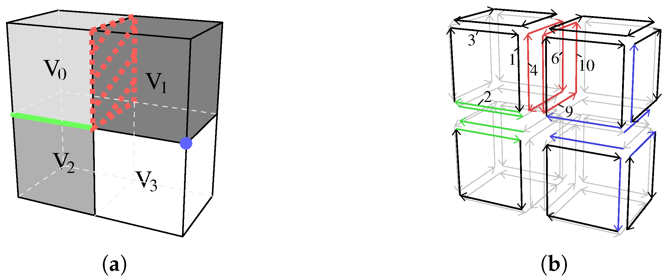
Illustration of a 3-map.Figure 1a shows an example of a 3D mesh composed of 4 volumes (, , ), 20 faces, 33 edges and 18 vertices. Note that and are adjacent; is incident to the red dashed face and to the green edge. To represent this 3D mesh with a 3-map, each volume is decomposed; then each face of the volumes is decomposed; then each edge of the faces is decomposed. The darts can be seen in the 3-map depicted in Figure 1b representing the 3D mesh of Figure 1a. Each dart is depicted by an oriented segment. At the end, the 3-map representing the 3D mesh has 96 darts (since each volume has 6 faces and each face has 4 edges, and thus, each volume is represented by 24 darts).
Adjacency relations. The adjacency relations of the n-map, which describe the topology of the nD object, are reported on the darts. n relations are defined for each dart d:
- gives the dart after d that belongs to the same j-cells as the j-cells of d, for all ;
- , with , gives the dart different from d that belongs to the same j-cells as the j-cell of d, for all , .
Intuitively, allows us to swap the current i-cell while keeping the other j-cells unchanged, . , with are involutions (an involution is a bijection equal to its inverse). In other words, given a dart d, we obtain d when applying twice. is not an involution but a permutation (a permutation is a bijection having the same set D as domain and codomain). denotes . This mapping gives the dart before d that belongs to the same j-cells than d, for all . At the end, an n-map is defined by the -tuple , i.e., a set D of darts plus the n mappings.
Composition property. One important property of n-maps, which guarantees the topological validity of the represented objects, links all pairs of and mappings, for : must be an involution. For example, when two volumes are glued together, they share an entire face. In other words, the two parts of the shared face must have the same number of darts (and thus the same number of vertices and edges), which is verified by ensuring that is an involution. This property must be satisfied for each dart of the n-map. As a consequence, operations that modify an n-map must ensure that the resulting n-map still satisfies this property.
Free darts. An n-map allows us to represent an nD object with boundaries. In such an object, some -cells belong to the border of the object, i.e., there is only one n-cell containing it. All the darts that belong to these -cells do not have darts linked with them by . These darts are said n-free; and are all linked by with a special value called ⌀.
Cells in n-maps. Cells are represented implicitly in an n-map by the darts and the mappings. Each i-cell, , is defined by the set of darts that can be reached from one of its darts by using all , . Things are a little bit different for 0-cells (vertices): each 0-cell is defined by the set of darts that can be reached from one of its darts by using all combinations of two different . Thanks to this definition of cells and the definition of adjacency and incidence relations, we are able to retrieve all the topological relations in a given n-map.
Illustration of the relations. Let us take a closer look at some parts of Figure 1. Figure 2a shows the part of the 3-map that represents . In this example, , and . Since is an involution, . Figure 2b shows the part of the 3-map around the face between and , where . Since is an involution, . All the darts of the 3-map shown in Figure 1b are 3-free, except the darts that belong to the four faces around the central edge. For example, darts 1, 2 and 3 are 3-free, while dart 4 is not 3-free. We can observe the composition property of 3-maps on Figure 2b. We can for example verify that and .
i-attributes. An n-map only describes the combinatorial part of an nD object, i.e., its subdivision in cells, and all the adjacency and incidence relations between the cells. This is usually not enough in many applications where it is required to have additional information associated with some cells. For example, we need the geometry of the object to visualize it. This can be done by associating a point of to each vertex of the n-map. More generally, it is possible to associate any information to any i-cell in an n-map by using the notion of i-attribute (for example a position to each vertex, a color to each face, or an id to some edges).
2.2. Adaptive Hexahedral Subdivision
A lot of subdivision schemes have been proposed to adapt meshes, as the use of an adaptive mesh has several advantages. For example we can refine only interesting parts of a mesh, which reduces memory space and computational cost for the parts where a precise description is not required. These subdivision schemes have been used for example in several finite element applications based on hexahedral meshes. The simpler and the most used subdivision scheme is the subdivision 1:8, which is the one used in this paper.
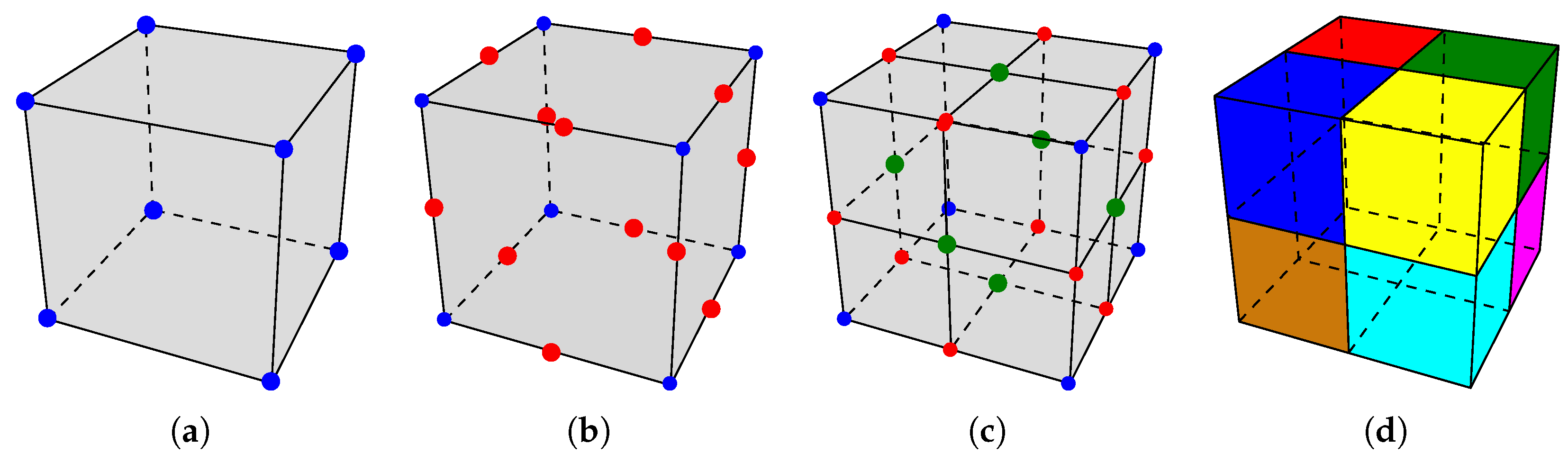
Subdivision 1:8. To subdivide a given hexahedron h (Figure 3a) in eight, the principle is the following: (1) split each edge of h in two (Figure 3b); (2) split each face of h in four (Figure 3c); (3) split h itself in eight (Figure 3d).
3-maps to represent hexahedral meshes. Using a 3-map to represent an irregular hexahedral mesh has several advantages. (1) We can represent any configuration of hexahedra: there is no constraint on the difference of subdivision level between two adjacent hexahedra; (2) We can use and mix different subdivision schemes. For example, we can split a hexahedron in two, four or eight; but it is easy to consider other types of subdivision; (3) We can retrieve and iterate through all cells of the mesh; and for each cell we can retrieve all its incident and adjacent cells; (4) Several operations exist and can be used to compute some characteristics (both geometrical and topological) and to modify the mesh; (5) Furthermore, we can mix different types of cells in the same mesh. For instance, we can describe and handle a mesh having hexahedra, tetrahedra, pyramids and prisms.
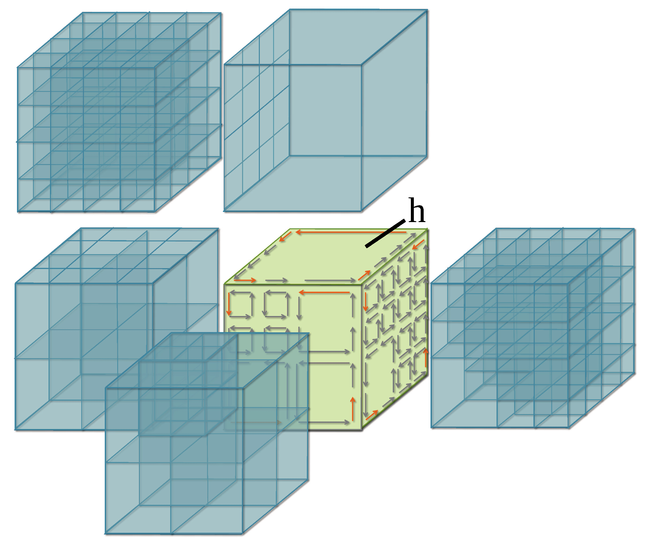
An adaptive subdivision method based on 3-maps. Given a hexahedral mesh represented by a 3-map, an adaptive subdivision method is given in [28] based on a 1:8 subdivision of the hexahedra. Note that it is possible to subdivide each hexahedron independently, while keeping the 3-map valid. More precisely, when a cell (edge or face) is split inside a hexahedron, corresponding cells inside adjacent hexahedra are subdivided accordingly in order to satisfy the property of 3-maps in the way that volumes are glued together. This is illustrated in Figure 4. The central hexahedron h is not yet subdivided. Anyway, since some of its neighbors are already subdivided, some cells incident to h were already split during these previous subdivisions. This is for example the case for some edges incident to the top face of h, and this is also the case for the face to the right of h. When subdividing h, it is possible to test which cells were already split or not (see [28]). Moreover, h can be subdivided correctly whatever the level of subdivision of the adjacent hexahedra of h are.
3. nD Distributed Combinatorial Maps
As we have just seen before, an n-map allows us to represent and to handle an nD object. This model has many advantages, given in the introduction of this paper, that justify its use. Anyway, it has two drawbacks: (1) algorithms on n-maps are sometimes difficult to parallelize; (2) memory space can prevent us from dealing with very big objects. In order to solve these drawbacks, our main contribution is the definition of nD Distributed Combinatorial Maps, called n-dmaps. The essential idea of this definition is to cut a given n-map into independent parts which can be processed in parallel, and possibly on different computers.
3.1. Definition of nD Distributed Combinatorial Maps
An nD distributed combinatorial map can be defined as a set of independent n-maps which are called blocks. In an n-dmap: (a) each n-cell belongs to exactly one block; as a consequence, links, for all i, are always defined between darts that belong to the same block; (b) some information is added for retrieving the links between two n-cells that belong to two different blocks. Definition 1 gives its mathematical definition.
Definition 1.
An nD distributed combinatorial map, , is a set of k independent n-maps and k labeling functions , . Each is a block of . The domains of functions are subsets . Each dart in is called a critical dart. satisfies the following properties:
- 1.
- must be a set of complete -cells, i.e., , all the darts of the -cell containing d must belong to ;
- 2.
- each dart in belongs to the border of , i.e., , d isn-free;
- 3.
- for each critical dart d in , there is exactly one critical dart in , with , such that . For all other critical darts in any block z, ;
- 4.
- for each pair of critical darts in blocks and such that : , .
Intuitively, a critical dart is a dart that is linked by to a dart belonging to a different block. Note that only critical darts have a label and this label is global for all the different blocks , (two different critical darts in a same block have two different labels, and only the two darts linked by between two different blocks have the same label). Property (4) ensures that the labeling of different critical darts are compatible inside the two -cells that are separated in two different blocks.
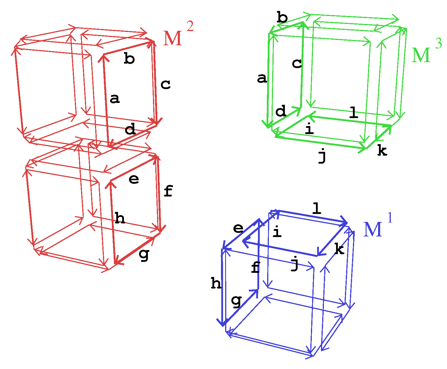
Illustration with an example.Figure 5 gives an example of a 3-dmap that represents the 3-map M of Figure 1b. has 3 blocks: containing two cubes; and containing one cube. Each block , has 8 critical darts (labeled with lowercase letters). Looking at the properties of critical darts:
- Property (1) can be verified as all critical darts of form complete faces of their block.
- Property (2) can be verified as all critical darts of belong to the border of their block; each one corresponds to one face in M which is split in two in .
- Property (3) can be verified by checking that all critical darts that were linked by in M have the same label in , and we can verify that other pairs of critical darts have different labels.
- Property (4) ensures that critical darts are labeled in a coherent way between the different blocks. In our example, critical darts of the top cube in block are labeled a, b, c, and d. Corresponding darts in block are also labeled a, b, c, and d. Starting from dart d labeled a in block and dart with the same label in block , we can check that darts and have the same label b. Step by step, this ensures the coherent labeling of all the darts of the two faces.
3.2. Retrieve Information Inside nD Distributed Combinatorial Maps
By using the definition of an nD distributed combinatorial map giving the properties satisfied by the blocks and the labeling function, it is possible to retrieve the global combinatorial map described by the different blocks without needing to rebuild it. This is detailed in Proposition 1 which defines the global n-map by: (1) the union of the sets of darts of all blocks; (2) , …, mappings are directly retrieved from the corresponding mappings in each block (indeed, by Definition 1 we are sure that two darts linked by these mappings always belong to the same block); (3) mapping is either retrieved from the same mapping in each block for non critical darts; and (4) retrieved from the labeling function otherwise.
Proposition 1.
Let be an nD distributed combinatorial map. The n-map described by is defined by:
- 1.
- 2.
- , , : ;
- 3.
- , : ;
- 4.
- , , let denote the dart in such that , , . Then, .
It is easy to verify that is a permutation on D, and that , …, are involutions. Indeed, all mappings are directly retrieved from the existing mappings in each block, except of critical darts. For this last case, by definition of the labeling function, we are sure that there exist only two darts and having the same label. Lastly, we can also verify that is an involution on D for any , . For this is obvious since and are directly taken from the same block, which is an n-map and thus satisfies this property. For , we can prove that is an involution by using Property (4) of Definition 1 (we know that , and implies ). This proves that M obtained by Proposition 1 is an n-map.
Illustration with an example. In the example given in Figure 5, it is easy to verify that and mappings are directly retrieved from the corresponding mappings in each block. For , darts describing the face between the two cubes in block are not critical, and thus have their links directly given by the links in . However, this is not true for critical darts describing for example the face between and . For example, dart labeled a in is critical. The only other dart labeled a belongs to block and we conclude that these two darts are linked by .
3.3. A Data Structure for Storing nD Distributed Combinatorial Maps
To store an n-dmap , any classical data structure for representing an n-map can be used to store each block of (see for example [29,30]). However, we need to represent additional information about critical darts in order to propose an efficient solution to retrieve links with a good complexity. Our solution is to store the following information in each block , , in addition to the classical data structure that represents the n-map:
- each critical dart is marked with a Boolean mark, and stores its label;
- one associative array gives for each label used in this block the critical dart d of with this label.
The Boolean mark allows us to test in constant time if a dart is critical or not. Each critical dart d directly stores its label, which can thus be retrieved in constant time. Moreover, the associative array allows us to retrieve the critical dart having a specific label (If we use a hash table for the associative array, retrieving a dart from its label can be done in amortized constant time.).
Note that each block is fully independent in this data structure, and there is no need for shared memory. This is the perfect solution to implement a parallel algorithm on different computers that communicate with message passing system, as we will see in our experiments.
Possibility to store block numbers of critical darts. It is possible to store in each critical dart the number of the other block sharing this label. This additional information can be used in order to optimize the communication between the tasks, because each block knows directly the other block that contains a given critical dart. It is then possible to send messages only to concerned blocks. In return, there is a small overhead in terms of memory space. Without this information, the memory space occupied is smaller, but messages must be broadcast. This possibility offers a compromise that can be used or not, depending on the priority of applications.
3.4. Extensions and Discussion
Our definition of distributed combinatorial maps has two strong properties: (1) each n-cell of the global combinatorial map belongs entirely to one block; (2) darts can not be duplicated in two (or more) different blocks.
The first property is important for Proposition 1 in order to show how it is possible to retrieve all the information of the global combinatorial map corresponding to a given distributed n-map. Moreover, n-cells usually carry important information of the mesh that are necessary in several applications. For this reason, it seems natural not to split an n-cell between different blocks. However, it is possible to relax this constraint, if needed, by modifying Definition 1, to have sets of critical darts, one per dimension of the n-dmap. A critical dart in dimension i will be linked by to the other critical dart in dimension i having the same label.
The second property implies that the set of darts of the different blocks forms a partition of the set of darts of the global combinatorial map. This avoids the need to apply a same operation several times when there are some duplicated parts of the mesh in several blocks. However, depending on applications, it could be useful to create some halo (or ghost) regions around cells of a given block. To do so, Definition 1 can be modified by adding a set of duplicated darts, one per block of the n-dmap. These darts can belong to different blocks, and must be labeled with a unique and global name (like for critical darts). When an operation modifies a duplicated dart in a given cluster, a message must be sent to all the clusters containing this dart in order to apply the same modification.
The complexity of several algorithms can be improved by using our distributed combinatorial maps, as illustrated in this paper for an adaptive hexahedral mesh refinement method. Generally speaking, all algorithms that can be split in independent computations will be improved. When there are few dependent parts, global consistency can be preserved by adding a few communications between blocks and in this case, the complexity is still improved. However, operations that have huge dependent parts, that require global computation of the entire mesh, will not be improved when applied on distributed combinatorial maps. Indeed, in such a case, a lot of messages will be sent, possibly with a lot of information to exchange between the different blocks. However, this is a well known limitation of parallel computing and our solution does not provide a magic solution to this problem. Moreover, we would like to remind that the first goal of distributed combinatorial maps is to enable dealing with huge maps that do not fit in the memory space of a single computer, and this goal is achieved as illustrated in our experiments.
4. A Parallel Algorithm of Mesh Processing Based on 3-dmaps
In this section, we illustrate the interest of using a distributed combinatorial map by proposing a parallel algorithm for mesh processing. For this purpose, we consider an adaptive hexahedral mesh refinement. Indeed, by using the independent blocks of an n-dmap, a parallel version of a mesh processing algorithm is simple to achieve. Moreover, critical darts in the n-dmap give us all information required to ensure the global consistency of the different blocks. This aspect is important to guarantee the same final result when using an n-dmap with a parallel process, as when using an n-map with the corresponding sequential process.
Many works exist on parallel mesh processing and adaptive hexahedral mesh refinement (see for example [31,32,33,34,35,36,37,38,39,40,41,42]) which shows the interest of this field of research. Several libraries are available that provide efficient parallel adaptive mesh refinement, for example libMesh [43] or PUMI [44]. However, these libraries are not generic, they are only defined in a fixed dimension, and do not allow us to consider any type of meshes. For example, authors of PUMI say in their paper: “the mesh must be composed of entities which belong to a small set of topological types…Regarding polyhedral meshes, it should be possible for the MDS structure to accept new topological types at runtime, though its performance will degrade as the number of types grows large. Good performance can be found using about 10 types or less, but when more than 100 types are involved, this may no longer be the optimal structure.” In libMesh, it is only possible to represent basic objects (hexahedron, tetrahedron, prism, pyramid).
Our goal in this paper is not to define a new method of parallel adaptive hexahedral mesh refinement better than previous works, but to illustrate the interest of our distributed combinatorial maps with a mesh processing example. Moreover, we remind that the main interest of our solution is to be generic. With our data structure, we can use many different algorithms to compute characteristics and to modify nD meshes, which is often not possible when using non generic data structures, for example allowing us only to represent some specific types of cells.
In Section 4.1, we start by giving a generic parallelization of the considered algorithm. This parallel algorithm can be executed in sequential or in parallel, with a multi-threaded version or a distributed version. This generic algorithm uses our distributed combinatorial maps, and uses messages to update critical darts in the different blocks. There are several possibilities in order to transfer messages between the block, two of them are given in Section 4.2.
4.1. Generic Parallel Algorithm
The considered algorithm is the adaptive hexahedral subdivision of a given 3D mesh. Considering a hexahedral mesh, the main principle is the following: (a) iterate through each hexahedron h of the mesh; (b) ask to an oracle if h must be subdivided or not; (c) if the answer is yes, subdivide h in 8 hexahedra (for a 1:8 subdivision). Note that this algorithm can not be accomplished by using half-edges data structure. Indeed, this model allows us only to describe surfaces (i.e., a set of faces glued together) embedded in 3D space, while the hexahedral subdivision method needs to represent volumes glued together.
This main principle can be retrieved in Algorithm 1 corresponding to one parallel task of our parallel algorithm. k tasks are run independently and simultaneously, one for each block of the 3-dmap, generating some communication (exchanging messages) between the different parallel tasks.
Looking at Algorithm 1, the first loop (line 1) iterates through each hexahedron h of the current block (corresponding to a part of the whole mesh). When h must be subdivided (this question is given to an oracle), we first split each edge of h in two (lines 3–10), then we split each face of h in four (lines 11–17). Then, h is split itself in eight hexahedra (line 18), and all the messages that has received are read and handled before considering the next hexahedron (line 19). Note that for each edge (resp. face) to split, we first test if the edge (resp. face) is already subdivided or not (line 4, resp. line 12). Indeed, one cell of h can be already subdivided in a previous step when considering a hexahedron adjacent to h. Note also that this could occur both for critical and non critical darts.
The principle of Algorithm 1 is very simple. The only difficult parts concern the critical darts management (lines 6–10 for edges; 15–17 for faces). Indeed, when a hexahedron has no critical dart, its subdivision is only local to its block and thus it can be done locally without any problem. However, when the hexahedron has some critical darts, additional work must be done to guarantee the global validity of the 3-dmap.
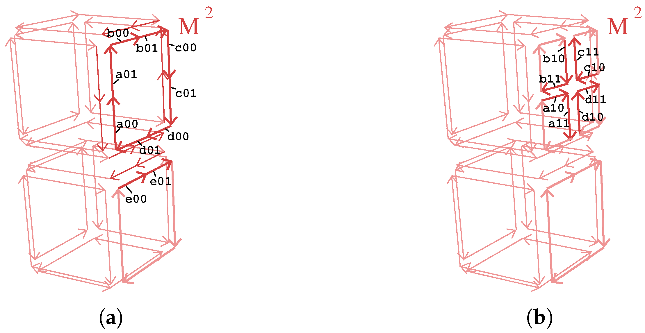
Management of critical darts. Let us focus on the division of a face f having critical darts e.g., the face with critical darts labeled a, …, d in Figure 5. The two steps of this division are shown in Figure 6. To split f, we need to:
| Algorithm 1: Hexahedral mesh refinement of a given block. |
 |
- split the four edges of f (line 5):
- -
- this splits the four critical darts labeled a, …, d;
- -
- the old darts are relabeled a00, …, d00 (line 9, cf. Figure 6a);
- -
- the new darts are labeled a01, …, d01 (line 10, cf. Figure 6a);
- -
- four messages are sent (line 8) in order to split also the corresponding edges in cluster (which is mandatory in order to preserve the global validity of the 3-dmap);
- split f in four (line 14):
- -
- the four corner darts of f are critical (by definition they are either all or none critical);
- -
- the message “split face” with the labels of the four corner darts as parameter is sent to , the other block containing the critical darts. This guarantees that each face matches in both blocks (line 16);
- -
- new darts created during the split of face f are all critical and are labeled in a unique way by using the label of the original darts of f (line 17, cf. Figure 6b to see how this labeling is done).
The special way that the labeling and re-labeling of critical darts is done ensures that the properties of distributed combinatorial maps are preserved. When splitting an edge, all the darts of the edge are split. As illustrated in Figure 6a, this can lead to splitting several critical darts. For each critical dart concerned by a split, a message is sent in order to perform the same modification in the other block having this critical dart. This message takes the label of the critical dart as parameter. Similarly, when splitting a face made of critical darts, the “split face” message is sent with the four labels of the four corner darts as parameter. The four labels are required in order to detect in the other block sharing this face if the face was already split or not.
Management of messages. At the end of Algorithm 1, when a hexahedron h has just been subdivided, messages sent from other blocks are read and handled (line 19). This is achieved in Algorithm 2. The main principle of this algorithm is to read all the messages that arrived in the message queue associated with block . There are only two different types of messages: “split edge” and “split face”. For both types of message, we split the corresponding cell, while using the same rules for labeling and re-labeling of critical darts as the rules used in Algorithm 1 in order to preserve the compatibility between labeling of different blocks. This guarantees the global consistency of the 3-dmap , since we apply exactly the same operations on the same cells in each different block of .
| Algorithm 2: Receive and handle all the messages of a given block. |
 |
Looking at Algorithm 2, before splitting an edge, we first test if the given label is still associated with a critical dart (line 3). This is done simply by testing if the given label still exists in the corresponding associative array of critical darts. Note that this step is required because a critical dart could have already been subdivided (if one incident hexahedron was subdivided) before receiving this message. If the dart has already been subdivided, there is nothing to do because the global consistency of is already correct. When the critical dart with the given label exists, we split the edge containing this dart (line 4), label and relabel critical darts (lines 8 and 9) and send the “split edge” message for each critical dart split (line 7).
We may wonder why we need to send the “split edge” message again. This is to correctly take into account the case where an edge in the initial 3-map is split into two (or more) edges in one block.
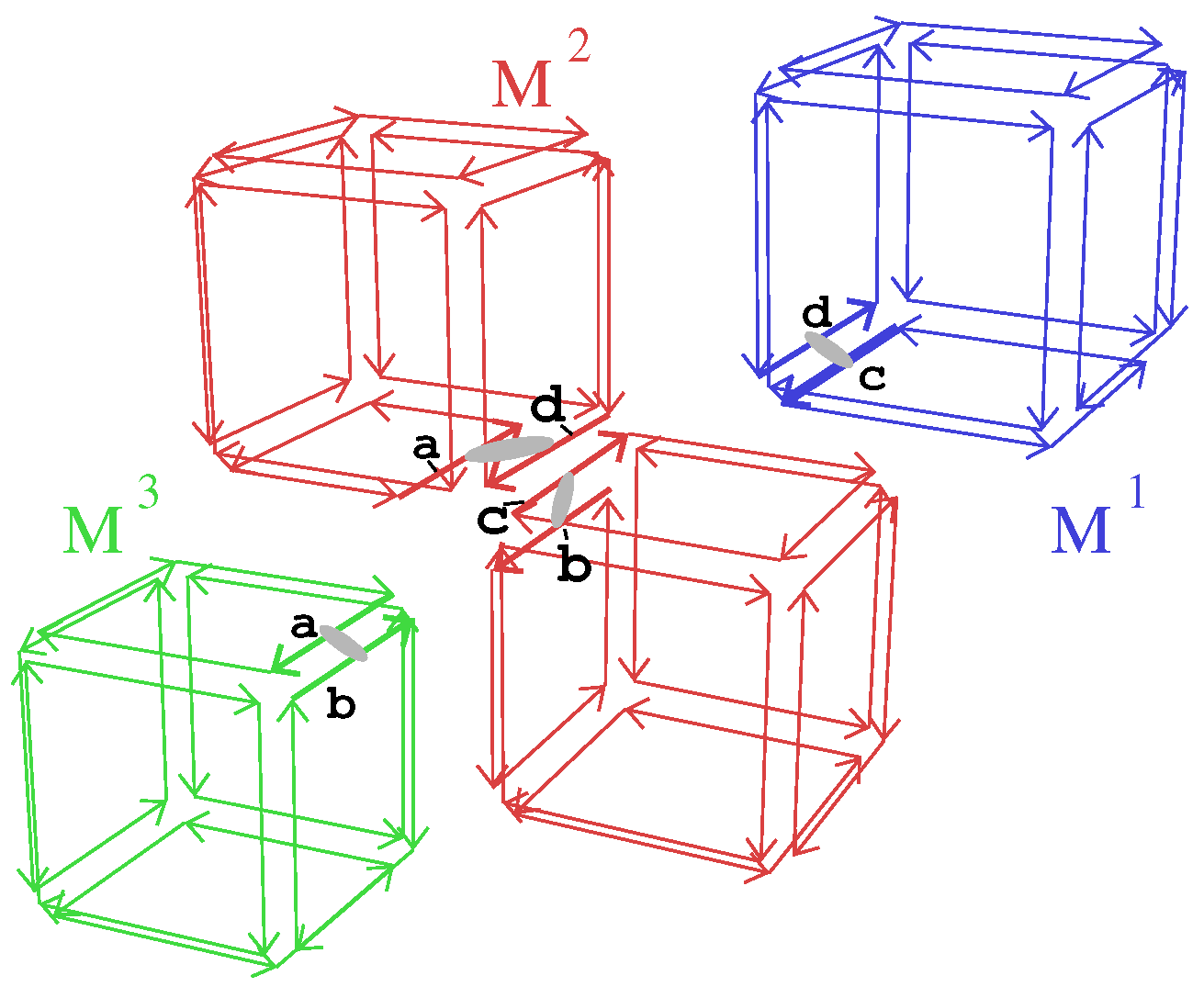
Such a case is illustrated in Figure 7. In this example, the central edge between the four cubes belongs to the 3 blocks , and is split in 2 edges in block . Indeed, in this block, there is no link between darts labeled a and d and darts labeled b and c (This is due to the definition of n-maps which allows us only to glue n-cells along (n-1)-cells.). In this example, let us suppose that the face containing the critical dart a should be split in four in block . Algorithm 1 starts to split the four edges of this face, and thus the face containing this critical dart. During this split, only critical darts labeled a and d are split since critical darts labeled b and c do not belong to the same edge in this block (even if they belong to the same edge in the global 3-map). Two “split edge” messages are sent for the two labels a and d. Block will receive the message for label a, and thus split the two critical darts labeled a and b, while block will receive the message for label d, and thus split the two critical darts labeled d and c. These two splits will generate a new “split edge” message for label c which will be received by block allowing us to split also the two critical darts b and c in this block.
Things are similar when receiving a “split face” message. We first test if the corresponding face is not yet split, by testing if the four given labels of the message belong to the same face (in this case the face is not yet subdivided) or not (in this case the face was already subdivided). When the face is not subdivided, we split it into four and label the new darts using the same rule as in Algorithm 1 (and illustrated in Figure 6). For this type of message, there is no need to send the “split face” message again because, by definition of 3-dmaps, we know that there is exactly two volumes incident to each critical face. Indeed, this block deals with the second volume, the first one was processed by the block having sent this message.
When all the messages in the waiting queue are processed, we go back to Algorithm 1 in order to possibly continue to subdivide another hexahedron.
Note that many other possibilities could be used instead of alternating the subdivision of a hexahedron and the treatment of the messages. For example, we could process messages only after all hexahedra were subdivided (but in this case the message queue could become very large); or process messages only after having subdivided a fixed number of hexahedra; or process messages when the message queue has more than a given number of messages, etc.
4.2. Message Passing
In order to transfer messages between the different blocks of the distributed combinatorial maps, we can either broadcast messages to everybody or send messages only to the concerned blocks.
- If we broadcast messages, each message is sent to all tasks. When receiving a message, a task must first test if it is concerned by the message or not. This test is achieved by searching the critical dart in the associative array of critical darts. Since this test must be done anyway (to know if the cell was already subdivided or not, cf. lines 3 and 11 in Algorithm 2), there is no overhead in complexity. The only additional cost is due to the communication: many messages could be exchanged.
- If we do not broadcast messages, we use the possibility introduced in Section 3.3 where each critical dart stores the number of the other block containing this critical dart. With this number, it is then possible to directly send a message to the concerned block. In this case, the number of messages sent is smaller, but there is a small overhead in memory space to store these block numbers.
5. Experiments
In this section, we discuss the implementation and results of a hexahedral subdivision of a mesh using 3D distributed combinatorial maps.
Given a polygon mesh of a closed orientable surface, we consider an initial coarse 3-dmap subdividing its bounding box into a small number of hexahedra. In this initial 3-dmap, the hexahedra are set in different blocks. Thus, our method has two parameters: the initial number of hexahedra, and the number of blocks k. In our implementation, we did not try to optimize the way in which hexahedra are assigned to blocks, but this could be interesting in order to maximize the distribution of work load on the different computers. Then, each hexahedron that is intersected by the polygon mesh is recursively subdivided into 8 sub-volumes. Algorithm 1 is used in parallel on k computers, one computer for each block of the 3-dmap. This recursive subdivision is executed until either the hexahedron is no more intersected by the surface, or a certain criterion is satisfied. As criterion, we use either a limit of the depth of subdivision, or a limit on the total memory space occupied by the process. Whatever the criterion used, hexahedra are subdivided by level: we consider all hexahedra at depth i before considering hexahedra at depth .
Finally, we remove all the hexahedra of the 3-dmap that are in the exterior of the mesh. To do so, the removal operation for 3-maps is used [45] for each hexahedron that is outside of the mesh. This operation erases all the darts of the given hexahedron. Darts previously linked by with these removed darts become 3-free. Thanks to the use of a distributed combinatorial map, these removals can be done simultaneously between the different blocks because they are independent (each volume is contained in a single block). When a critical dart is removed in one block, a message is sent to indicate that this dart is no more critical in the other block.
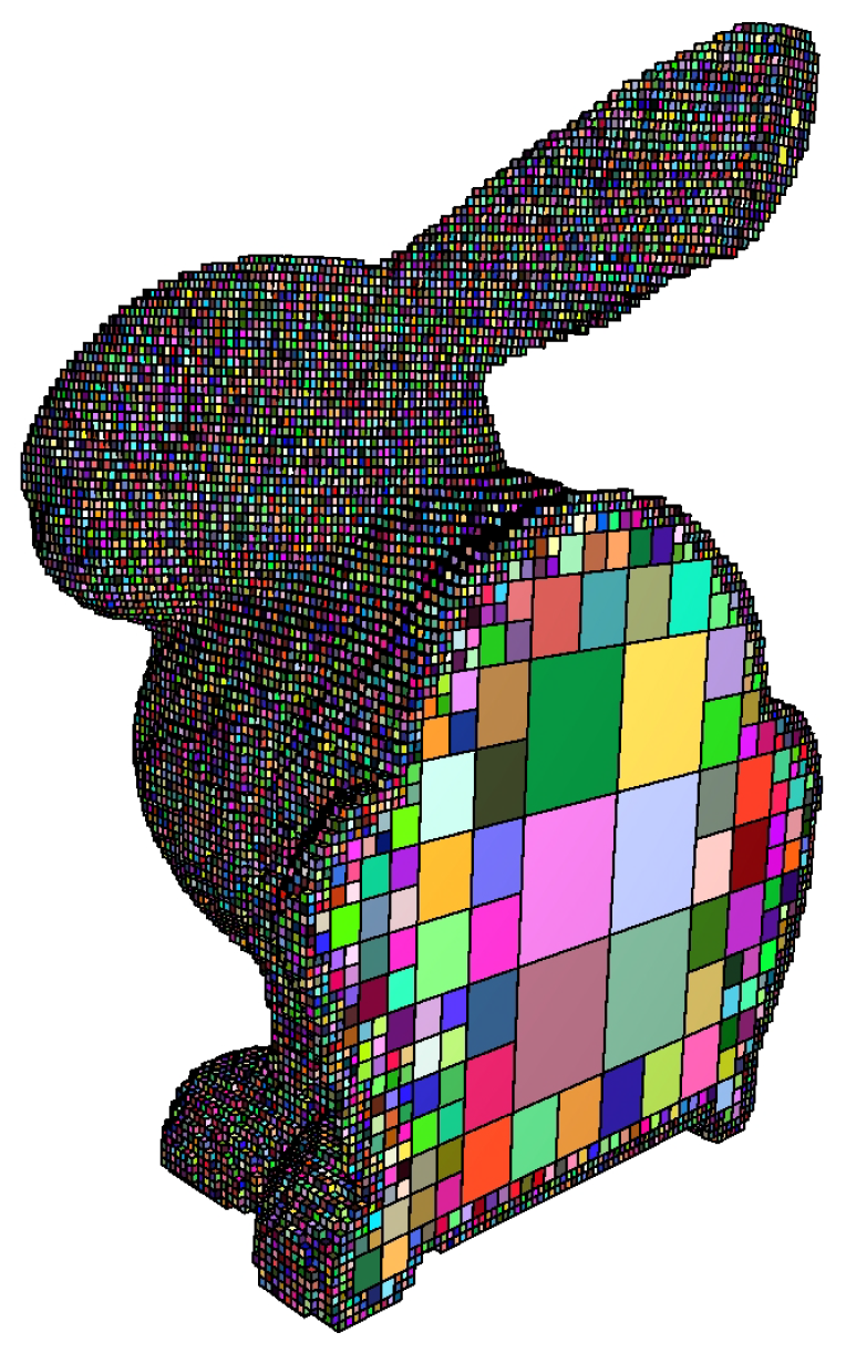
At the end of this process, the resulting 3-dmap represents an octree of the interior of the mesh, as illustrated in Figure 8.
Our distributed combinatorial maps were implemented in C++ using the Cgal library [46]. Each block was stored by using the combinatorial map package [27]. The intersection test was performed using the efficient axis-aligned bounding boxes (AABB) tree. An AABB tree is a static data structure that stores a set of geometric objects, and that allows us to perform efficient intersection and distance queries against these objects [47]. Our goal is to integrate our implementation of distributed combinatorial maps in a future release of Cgal.
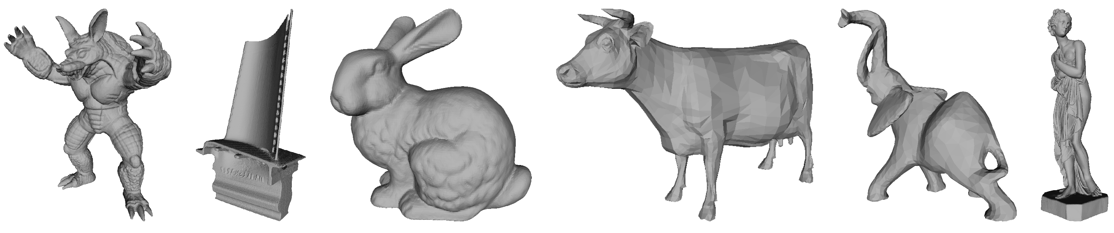
For our experiments, we used six different polygon meshes (usually considered in computer graphics). These polygon meshes are depicted in Figure 9, where we give their number of faces. In all our experiments, we used the same number of initial hexahedra, given in the array below Figure 9.
We implemented a parallel version of our subdivision and hexahedral removal algorithms by using independent processes, one per block of the distributed combinatorial map, using OpenMPI (MPI stands for “Message Passing Interface”) to transfer messages, and used mpirun to execute parallel jobs in different computers [48].
Our software was executed on the grid engine at the IN2P3 computing center https://cc.in2p3.fr/en/, on a system made of 16 workers, each one having 32 “Intel(R) Xeon(R) CPU E5-2698 v3 @ 2.30GHz” processors; with 128 GB memory for each worker. On this grid, the limit of parallel processes allowed to be run in parallel is 32, and each process is allowed to use at most 3 GB of memory.
5.1. Choice of the Communication Method
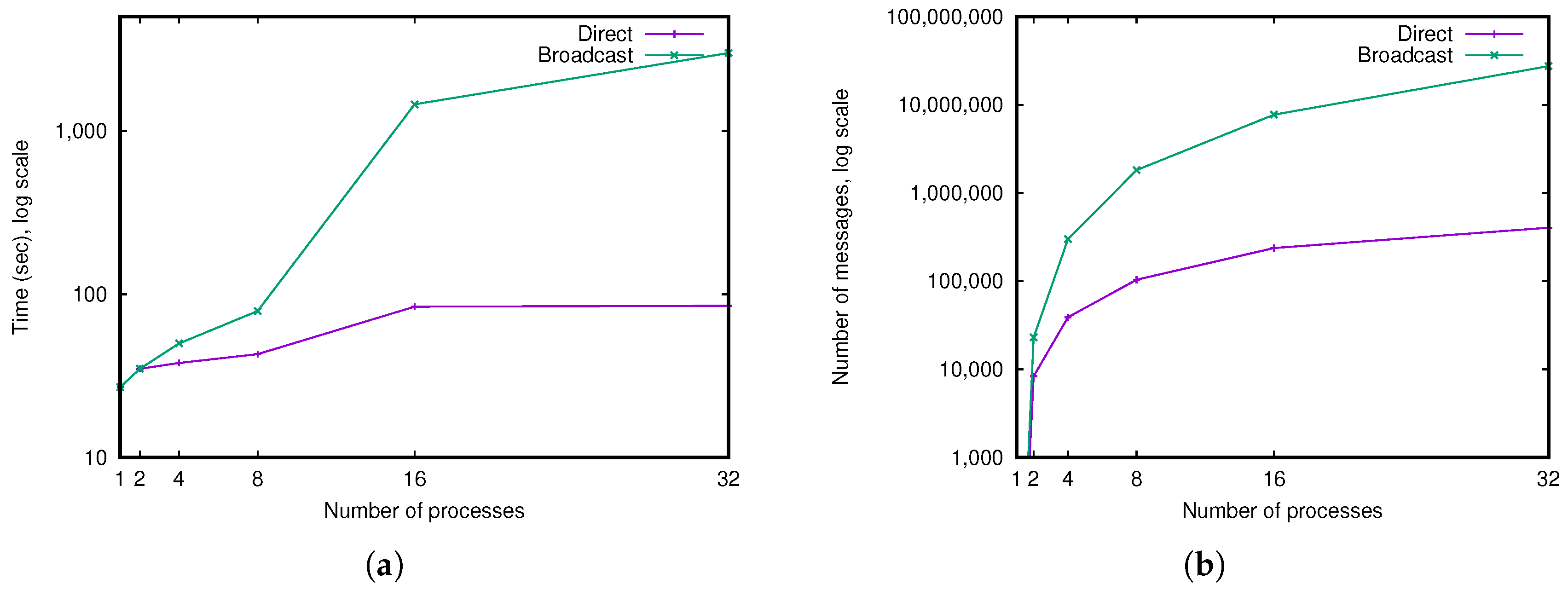
We conducted a first experiment in order to compare the two possible communication methods explained in Section 4.2. The “Broadcast” method, where each message is sent to all other processes, and the “Direct” method, where each message is sent only to the other concerned process. In this experiment, we fixed a memory limit to 1 gigabyte per process, and ran our software by increasing the number of processes from 1 to 32, a first time with the “Broadcast” method, and a second time with the “Direct” method.
We can see in Figure 10 the overall computation time and number of messages sent for both methods (curves give the average for our six meshes). When comparing the computation time, we can see that the “Direct” method is much faster than the “Broadcast” method, when the number of processes increases. Indeed, for 32 processes, the average computation time is 85 s for “Direct”, while the computation time is 3000 s for “Broadcast”.
For a small number of processes (less than or equal to 8), we can observe that both methods are more or less equivalent. Indeed, in these cases, the number of exchanged messages is small implying only small differences in computation times. On the contrary, for a big number of processes, we can see that the computation time for “Broadcast” is totally dominated by the cost of the message passing.
The conclusion of this experiment is obvious: the “Direct” method is much better than the “Broadcast” one and thus we use only this “Direct” method in all following experiments.
5.2. Comparison in Computation Time
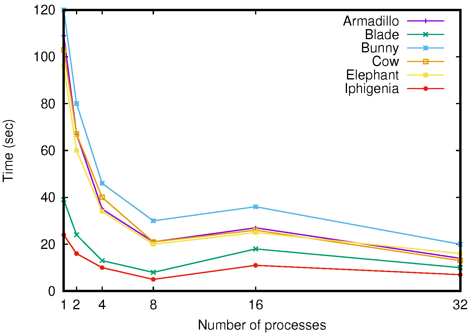
In a second experiment, we studied the computation time depending on the number of processes. To do so, we fixed a depth limit for each mesh, and ran our software by increasing the number of processes from 1 to 32. Using the same depth limit for each run implies doing exactly the same subdivision whatever the number of processes, and thus all the final 3-dmaps, and the corresponding 3-maps, are equal. For 1 process, we use the non distributed version of combinatorial maps provided in Cgal [27].
The depth limits were respectively equal to 5, 4, 5, 5, 5 and 4 for the different meshes Armadillo, Blade, Bunny, Cow, Elephant and Iphigenia. We chose these limits in order to respect the memory limit of 3 gigabytes per process allowed by the IN2P3 computing center.
We can see in Figure 11 the overall computation time of our subdivision method, depending on the number of processes, for each mesh. On average, the method takes 82 s for one process, and 13 s for 32 processes. The speedup is thus about . This time saving is interesting, even if we are far from the maximal possible speedup of 32. This difference is explained by the cost of the message passing.
We can probably improve our results by using classical optimization used in parallel algorithms, for example by using message grouping, or by optimizing the clustering of initial hexahedra in order to decrease the number of critical darts and thus the number of messages sent.
We recall that improving the computation time is not the main goal of this work: our main goal is to be able to deal with big 3-maps that do not fit in the memory of a single computer. For this reason, the speedup of is good enough for our method which does not use any specific optimization, and we did a last experiment in order to study how the memory space of the 3-dmap evolves depending on the number of processes.
5.3. Comparison in Memory Space
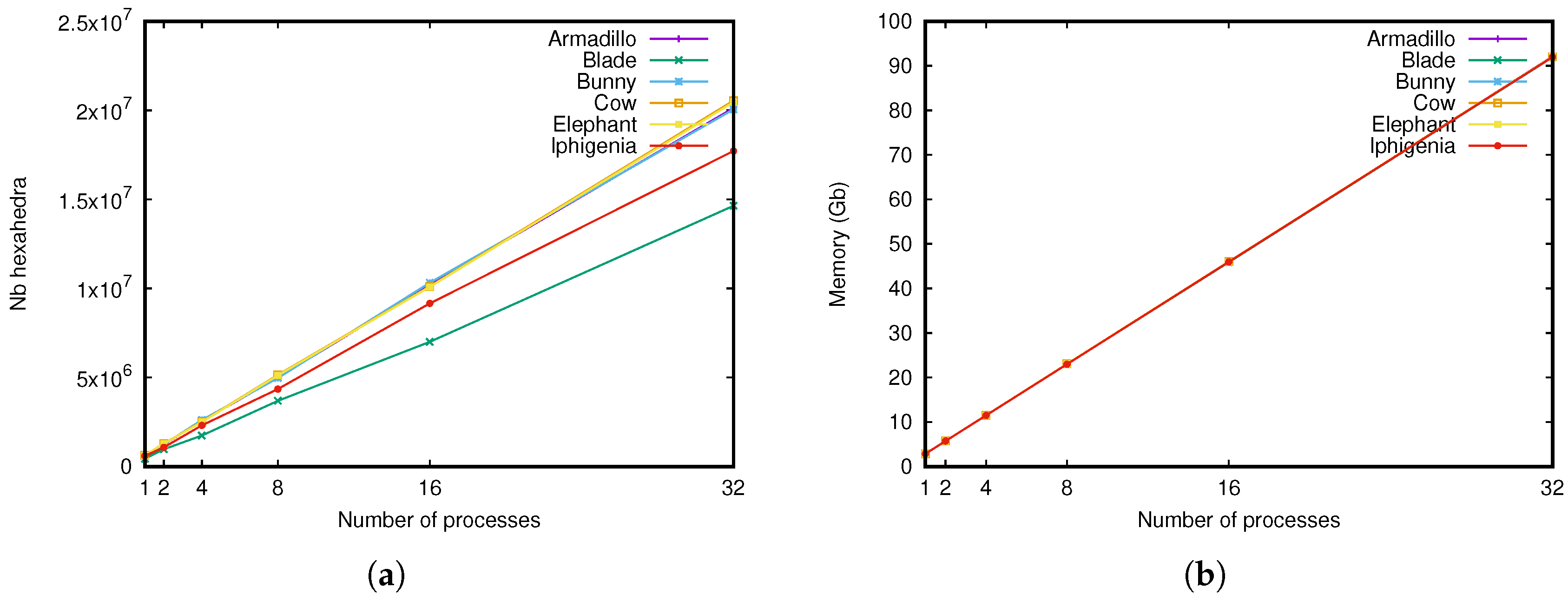
In this third experiment, we studied the number of hexahedra and the memory space of the 3-dmap depending on the number of processes. In this experiment, we fixed a memory limit to 3 gigabytes per process (the maximum value allowed by the IN2P3 computing center), and ran our software by increasing the number of processes from one to 32.
Results can be seen in Figure 12. As we can observe in Figure 12a, the number of hexahedra obtained in the final 3-dmap increases with the number of processes. Indeed, the limit of 3 gigabytes fixed by the IN2P3 is per process: using a distributed combinatorial map in k processes allows us to use gigabytes of memory, and thus allows us to store much more hexahedra.
On average for the six meshes, we could store 599,720 hexahedra with one process, and 18,925,061 with 32 processes: we were able to store about more hexahedra. This shows that the memory space overhead due to additional storage for the distributed combinatorial map is negligible comparing to the memory space for the different 3-maps.
Comparing the memory space of the final 3-dmap, given in Figure 12b, confirms this result: with 32 processes, we are able to use gigabytes of memory.
The overall computation times of our method were respectively 115, 145, 158, 176, 291 and 292 s (average for the six meshes). The program run with 32 processes was about slower than the program run with one process; however, this is a very good improvement knowing that we computed about more hexahedra. This can be verified by comparing the computation time per 100,000 hexahedra. These times were respectively 19, 12, 7, 4, 3 and 2 s, showing a speedup of about 9.
These results show that our method can be used to generate very big meshes due to our distributed combinatorial maps, and we will probably be able to deal with much bigger meshes by running more processes.
This experiment shows that the main goal of this paper is clearly reached: with our distributed combinatorial maps, it is now possible to handle big objects that do not fit in the memory of a single computer. We are able to apply an operation on the 3-dmap and obtain the same result as if we had used a classical 3-map on a single computer with a huge memory space.
6. Conclusions
In this paper, the main contribution is the definition of nD distributed combinatorial maps. Its main idea is simple: cut an n-map in independent blocks and add some information to link the different parts and retrieve information at the interfaces. Our solution has two main advantages: (1) it simplifies the implementation of parallel mesh processing algorithms; (2) it allows us to represent very big nD meshes that do not fit in the memory of a single computer.
In this paper, we have shown how to retrieve all the information of the global n-map without needing to recompute it. Thanks to this possibility, we can navigate through an n-dmap stored in several computers as if it was a big n-map stored in a single computer. This possibility is very interesting and opens many perspectives in order to develop new mesh processing methods that work on very big meshes. Note that since a 2-map is equivalent to a half-edge data structure, our solution can be used in 2D in order to store and handle 2D distributed half-edges.
As future work, we would like to study other types of parallel architectures, for example GPUs. We would also like to improve our partitioning in order to try to obtain similar workloads for each task while minimizing critical darts. To do so, we need to propose a cell migration method that allows us to transfer some cells between the different blocks. We would also like to study if it is possible to use the compact representation of hierarchical meshes [49] with our distributed version. This could reduce again the memory space occupied by each block. Lastly, we would like to develop other mesh processing algorithms based on our distributed combinatorial maps, and use them in different applications for example in an adaptive mesh refinement simulation. We would also like to develop applications in higher dimension, which is directly possible as a result of our generic definition of distributed combinatorial maps.
Author Contributions
Conceptualization, G.D.; Methodology, G.D.; Software, G.D.; Validation, G.D.; Writing—Original Draft Preparation, G.D., A.G.-L., F.Z., F.D.; Writing—Review & Editing, G.D., A.G.-L., F.Z., F.D.
Funding
This research was funded by the European Union’s Horizon 2020 Research and Innovation program under the Marie Sklodowska-Curie Actions grant number 659526.
Conflicts of Interest
The authors declare no conflict of interest.
References
- Botsch, M.; Kobbelt, L.; Pauly, M.; Alliez, P.; Levy, B. Polygon Mesh Processing; AK Peters: Natick, MA, USA, 2010. [Google Scholar]
- Bajaj, C.L.; Schaefer, S.; Warren, J.D.; Xu, G. A subdivision scheme for hexahedral meshes. Vis. Comput. 2002, 18, 343–356. [Google Scholar] [CrossRef] [Green Version]
- Wu, J.; Westermann, R.; Dick, C. Physically-Based Simulation of Cuts in Deformable Bodies: A Survey; Eurographics (State of the Art Reports); Eurographics Association: Hoboken, NJ, USA, 2014; pp. 1–19. [Google Scholar]
- Döllner, J.; Buchholz, H. Continuous Level-of-detail Modeling of Buildings in 3D City Models. In Proceedings of the 13th GIS ’05 Annual ACM International Workshop on Geographic Information Systems, Bremen, Germany, 4–5 November 2005; ACM: New York, NY, USA, 2005; pp. 173–181. [Google Scholar]
- Sharir, M. Arrangements in higher dimensions: Voronoi diagrams, motion planning, and other applications. In Algorithms and Data Structures; Akl, S.G., Dehne, F., Sack, J.R., Santoro, N., Eds.; Springer: Berlin/Heidelberg, Germany, 1995; pp. 109–121. [Google Scholar]
- Arroyo Ohori, K.; Ledoux, H.; Stoter, J. Modelling and manipulating spacetime objects in a true 4D model. J. Spat. Inf. Sci. 2017, 14, 61–93. [Google Scholar]
- Liu, J.; Zhang, X.; Zhang, X.; Zhao, H.; Gao, Y.; Thomas, D.; Low, D.A.; Gao, H. 5D respiratory motion model based image reconstruction algorithm for 4D cone-beam computed tomography. Inverse Probl. 2015, 31, 115007. [Google Scholar] [CrossRef]
- Baumgart, B.G. A polyhedron representation for computer vision. In Proceedings of the American Federation of Information Processing Societies: 1975 National Computer Conference, Anaheim, CA, USA, 19–22 May 1975; pp. 589–596. [Google Scholar]
- Weiler, K. Edge-based data structures for solid modelling in curved-surface environments. Comput. Graph. Appl. 1985, 5, 21–40. [Google Scholar] [CrossRef]
- Mäntylä, M. An Introduction to Solid Modeling; Computer Science Press: New York, NY, USA, 1988. [Google Scholar]
- De Berg, M. Computational Geometry: Algorithms and Applications, 2nd ed.; Springer: Berlin, Germany, 2000. [Google Scholar]
- Guibas, L.J.; Stolfi, J. Primitives for the Manipulation of General Subdivisions and Computation of Voronoi Diagrams. ACM Trans. Graph. 1985, 4, 74–123. [Google Scholar] [CrossRef]
- Weiler, K. The radial edge structure: A topological representation for non-manifold geometric boundary modeling. In Geometric Modeling for CAD Applications; Elsevier Science: New York, NY, USA, 1988; pp. 217–254. [Google Scholar]
- Rossignac, J. 3D Compression Made Simple: Edgebreaker with Zip&Wrap on a Corner-Table. In Proceedings of the 2001 International Conference on Shape Modeling and Applications (SMI 2001), Genoa, Italy, 7–11 May 2001; p. 278. [Google Scholar]
- Edmonds, J. A Combinatorial Representation for Polyhedral Surfaces. Not. Am. Math. Soc. 1960, 7, 646. [Google Scholar]
- Tutte, W. A census of planar maps. Canad. J. Math. 1963, 15, 249–271. [Google Scholar] [CrossRef]
- Jacques, A. Constellations et graphes topologiques. Proc. Comb. Theory Appl. 1970, 2, 657–673. [Google Scholar]
- Ringel, G. Map Color Theorem; Springer: Berlin, Germany, 1974. [Google Scholar]
- Dobkin, D.; Laszlo, M. Primitives for the Manipulation of Three-Dimensional Subdivisions. In Proceeding of the Symposium on Computational Geometry, Waterloo, ON, Canada, 8–10 June 1987; pp. 86–99. [Google Scholar]
- Lopes, H.; Tavares, G. Structural Operators for Modeling 3-manifolds. In Proceeding of the ACM Symposium on SMA ’97 Solid Modeling and Applications, Atlanta, GA, USA, 14–16 May 1997; ACM: New York, NY, USA, 1997; pp. 10–18. [Google Scholar]
- Kremer, M.; Bommes, D.; Kobbelt, L. OpenVolumeMesh - A Versatile Index-Based Data Structure for 3D Polytopal Complexes. In Proceeding of the of 21st International Meshing Roundtable; Jiao, X., Weill, J.C., Eds.; Springer: Berlin, Germany, 2012; pp. 531–548. [Google Scholar]
- Dyedov, V.; Ray, N.; Einstein, D.R.; Jiao, X.; Tautges, T.J. AHF: Array-based half-facet data structure for mixed-dimensional and non-manifold meshes. Eng. Comput. Lond. 2015, 31, 389–404. [Google Scholar] [CrossRef]
- Edelsbrunner, H. Algorithms in Combinatorial Geometry. In EATCS Monographs on Theoretical Computer Science; Brauer, W., Rozenberg, G., Salomaa, A., Eds.; Springer: Berlin, Germany, 1987. [Google Scholar]
- Rossignac, J.; O’Connor, M. SGC: A Dimension-Independant Model for Pointsets with Internal Structures and Incomplete boundaries. In Proceedings of the Geometric Modeling for Product Engineering: Selected and Expanded Papers from the IFIP WG 5.2/NSF Working Conference on Geometric Modeling, Rensselaerville, NY, USA, 18–22 September 1989; pp. 145–180. [Google Scholar]
- Lienhardt, P. N-Dimensional Generalized Combinatorial Maps and Cellular Quasi-Manifolds. Int. J. Comput. Geometry Appl. 1994, 4, 275–324. [Google Scholar] [CrossRef]
- Damiand, G.; Lienhardt, P. Combinatorial Maps: Efficient Data Structures for Computer Graphics and Image Processing; AK Peters: Natick, MA, USA; CRC Press: Boca Raton, FL, USA, 2014. [Google Scholar]
- Damiand, G. Combinatorial Maps. In CGAL User and Reference Manual, 3.9th ed.; CGAL Editorial Board, 2011; Available online: http://www.cgal.org/Pkg/CombinatorialMaps (accessed on 12 July 2018).
- Fléchon, E.; Zara, F.; Damiand, G.; Jaillet, F. A Unified Topological-Physical Model for Adaptive Refinement. In Proceedings of the 11th Workshop on Virtual Reality Interaction and Physical Simulation (VRIPHYS), Bremen, Germany, 24–25 September 2014; The Eurographics Association: Bremen, Germany, 2014; pp. 39–48. [Google Scholar]
- Kraemer, P.; Untereiner, L.; Jund, T.; Thery, S.; Cazier, D. CGoGN: n-dimensional Meshes with Combinatorial Maps. In Proceedings of the 22nd IMR 2013, International Meshing Roundtable, Orlando, FL, USA, 13–16 October 2013; pp. 485–503. [Google Scholar]
- Damiand, G.; Teillaud, M. A Generic Implementation of dD Combinatorial Maps in CGAL. In Proceedings of the 23rd International Meshing Roundtable (IMR), London, UK, 12–15 October 2014; Elsevier: London, UK, 2014; Volume 82, pp. 46–58. [Google Scholar]
- De Cougny, H.; Shephard, M. Parallel volume meshing using face removals and hierarchical repartitioning. Comput. Methods Appl. Mech. Eng. 1999, 174, 275–298. [Google Scholar] [CrossRef]
- Coupez, T.; Digonnet, H.; Ducloux, R. Parallel meshing and remeshing. Appl. Math. Model. 2000, 25, 153–175. [Google Scholar] [CrossRef]
- Chrisochoides, N. Parallel Mesh Generation. In Numerical Solution of Partial Differential Equations on Parallel Computers; Bruaset, A.M., Tveito, A., Eds.; Springer: Berlin/Heidelberg, Germany, 2006; pp. 237–264. [Google Scholar]
- Freitas, M.O.; Wawrzynek, P.A.; Neto, J.B.C.; Vidal, C.A.; Martha, L.F.; Ingraffea, A.R. A distributed-memory parallel technique for two-dimensional mesh generation for arbitrary domains. Adv. Eng. Softw. 2013, 59, 38–52. [Google Scholar] [CrossRef]
- Löhner, R. Recent Advances in Parallel Advancing Front Grid Generation. Arch. Comput. Methods Eng. 2014, 21, 127–140. [Google Scholar] [CrossRef]
- Ghisi, I.T.; Camata, J.J.; Coutinho, A.L.G.A. Impact of tetrahedralization on parallel conforming octree mesh generation. Int. J. Numer. Methods Fluids 2014, 75, 800–814. [Google Scholar] [CrossRef]
- Zhao, D.; Chen, J.; Zheng, Y.; Huang, Z.; Zheng, J. Fine-grained parallel algorithm for unstructured surface mesh generation. Comput. Struct. 2015, 154, 177–191. [Google Scholar] [CrossRef]
- Diachin, L.F.; Hornung, R.; Plassmann, P.; Wissink, A. Parallel Adaptive Mesh Refinement. In Parallel Processing for Scientific Computing; Heroux, M.A., Raghavan, P., Simon, H.D., Eds.; SIAM: Portland, OR, USA, 2006; Chapter 8; pp. 143–162. [Google Scholar]
- Freitas, M.O.; Wawrzynek, P.A.; Neto, J.B.C.; Vidal, C.A.; Carter, B.J.; Martha, L.F.; Ingraffea, A.R. Parallel generation of meshes with cracks using binary spatial decomposition. Eng. Comput. (Lond.) 2016, 32, 655–674. [Google Scholar] [CrossRef]
- Tautges, T.J.; Kraftcheck, J.; Bertram, N.; Sachdeva, V.; Magerlein, J. Mesh Interface Resolution and Ghost Exchange in a Parallel Mesh Representation. In Proceedings of the 26th IEEE International Parallel and Distributed Processing Symposium Workshops & PhD Forum, IPDPS 2012, Shanghai, China, 21–25 May 2012; pp. 1670–1679. [Google Scholar]
- Langer, A.; Lifflander, J.; Miller, P.; Pan, K.; Kalé, L.V.; Ricker, P.M. Scalable Algorithms for Distributed-Memory Adaptive Mesh Refinement. In Proceedings of the IEEE 24th International Symposium on Computer Architecture and High Performance Computing, SBAC-PAD 2012, New York, NY, USA, 24–26 October 2012; pp. 100–107. [Google Scholar]
- Ray, N.; Grindeanu, I.; Zhao, X.; Mahadevan, V.; Jiao, X. Array-based, parallel hierarchical mesh refinement algorithms for unstructured meshes. Comput. Aided Des. 2017, 85, 68–82. [Google Scholar] [CrossRef]
- Kirk, B.S.; Peterson, J.W.; Stogner, R.H.; Carey, G.F. libMesh: A C++ library for parallel adaptive mesh refinement/coarsening simulations. Eng. Comput. (Lond.) 2006, 22, 237–254. [Google Scholar] [CrossRef]
- Ibanez, D.A.; Seol, E.S.; Smith, C.W.; Shephard, M.S. PUMI: Parallel Unstructured Mesh Infrastructure. ACM Trans. Math. Softw. 2016, 42, 17:1–17:28. [Google Scholar] [CrossRef]
- Damiand, G.; Lienhardt, P. Removal and Contraction for N-Dimensional Generalized Maps. In Proceedings of the 11th International Conference on Discrete Geometry for Computer Imagery (DGCI), Naples, Italy, 19–21 November 2003; Lecture Notes in Computer Science. Springer: Berlin, Germany, 2003; Volume 2886, pp. 408–419. [Google Scholar]
- The CGAL Project. CGAL User and Reference Manual; CGAL Editorial Board: Boston, MA, USA, 2009; Available online: http://www.cgal.org/ (accessed on 12 July 2018).
- Alliez, P.; Tayeb, S.; Wormser, C. 3D Fast Intersection and Distance Computation. In CGAL User and Reference Manual, 3.5th ed.; CGAL Editorial Board: Boston, MA, USA, 2009; Available online: http://www.cgal.org/Pkg/AABB_tree (accessed on 12 July 2018).
- Gabriel, E.; Fagg, G.E.; Bosilca, G.; Angskun, T.; Dongarra, J.J.; Squyres, J.M.; Sahay, V.; Kambadur, P.; Barrett, B.; Lumsdaine, A.; et al. Open MPI: Goals, Concept, and Design of a Next Generation MPI Implementation. In Proceedings of the 11th European PVM/MPI Users’ Group Meeting, Budapest, Hungary, 19–22 September 2004; pp. 97–104. [Google Scholar]
- Untereiner, L.; Kraemer, P.; Cazier, D.; Bechmann, D. CPH: A Compact Representation for Hierarchical Meshes Generated by Primal Refinement. Comput. Graph. Forum 2015, 34, 155–166. [Google Scholar] [CrossRef] [Green Version]
Figure 1.
(a) A 3D mesh composed of 4 cubes, , , , two by two adjacent; (b) The corresponding 3-map having 96 darts (24 for each cube) where some darts are numbered.
Figure 1.
(a) A 3D mesh composed of 4 cubes, , , , two by two adjacent; (b) The corresponding 3-map having 96 darts (24 for each cube) where some darts are numbered.

Figure 2.
Two parts of the 3-map illustrated in Figure 1b, where some darts are numbered. (a) Cube representing . (b) Face between and .
Figure 2.
Two parts of the 3-map illustrated in Figure 1b, where some darts are numbered. (a) Cube representing . (b) Face between and .

Figure 3.
Hexahedral subdivision 1:8. (a) Initial hexahedron. (b) Split each edge in two. (c) Split each face in four. (d) Split the hexahedron in eight.
Figure 3.
Hexahedral subdivision 1:8. (a) Initial hexahedron. (b) Split each edge in two. (c) Split each face in four. (d) Split the hexahedron in eight.

Figure 4.
Illustration of a configuration that can occur when using an adaptive subdivision in a hexahedral mesh (image from [28]).
Figure 4.
Illustration of a configuration that can occur when using an adaptive subdivision in a hexahedral mesh (image from [28]).

Figure 5.
A 3-dmap that represents the 3-map of Figure 1b which has been decomposed into 3 blocks . Critical darts are labeled with lowercase letters a, …, l, and are drawn in bold.
Figure 5.
A 3-dmap that represents the 3-map of Figure 1b which has been decomposed into 3 blocks . Critical darts are labeled with lowercase letters a, …, l, and are drawn in bold.

Figure 6.
Block of the 3-dmap shown in Figure 5, for the two steps of the division of the face with critical darts labeled a, …, d. (a) After the split of the four edges. (b) After the split of the face.
Figure 6.
Block of the 3-dmap shown in Figure 5, for the two steps of the division of the face with critical darts labeled a, …, d. (a) After the split of the four edges. (b) After the split of the face.

Figure 7.
A 3-dmap composed of 3 blocks also representing the 3-map of Figure 1b. The central edge between the four cubes belongs to the 3 blocks , and is split in 2 edges in block .
Figure 7.
A 3-dmap composed of 3 blocks also representing the 3-map of Figure 1b. The central edge between the four cubes belongs to the 3 blocks , and is split in 2 edges in block .

Figure 8.
A block of a 3-dmap obtained by the hexahedral subdivision of Bunny. We can see hexahedra with different levels of subdivision.
Figure 8.
A block of a 3-dmap obtained by the hexahedral subdivision of Bunny. We can see hexahedra with different levels of subdivision.

Figure 9.
Initial polygon meshes used in our experiments. # faces is the number of faces of the original polygon meshes. # init. hexa is the number of hexahedra in the initial coarse 3-dmap.
Figure 9.
Initial polygon meshes used in our experiments. # faces is the number of faces of the original polygon meshes. # init. hexa is the number of hexahedra in the initial coarse 3-dmap.

| Mesh | Armadillo | Blade | Bunny | Cow | Elephant | Iphigenia |
| # faces | 52000 | 1765388 | 52000 | 5804 | 5558 | 703512 |
| # init. hexa |
Figure 10.
Comparison of two possible communication methods, for increasing number of processes (from 1 to 32). “Direct”: messages are sent directly to concerned blocks; “Broadcast”: messages are sent to all processes. (a) Total computation time, in seconds, average for the six meshes. (b) Number of messages exchanged, average for the six meshes.

Figure 11.
Comparison of global computation time (in seconds) to compute the same final hexahedral subdivision, for increasing number of processes.
Figure 11.
Comparison of global computation time (in seconds) to compute the same final hexahedral subdivision, for increasing number of processes.

Figure 12.
Comparison of maximal number of hexahedra and memory space occupied when using a 3-dmap for different number of processes. (a) Final number of hexahedra. (b) Maximal memory space occupied (in gigabytes). The six curves are superposed, because all runs occupy the same maximum memory space.

© 2018 by the authors. Licensee MDPI, Basel, Switzerland. This article is an open access article distributed under the terms and conditions of the Creative Commons Attribution (CC BY) license (http://creativecommons.org/licenses/by/4.0/).
Share and Cite
MDPI and ACS Style
Damiand, G.; Gonzalez-Lorenzo, A.; Zara, F.; Dupont, F. Distributed Combinatorial Maps for Parallel Mesh Processing. Algorithms 2018, 11, 105. https://doi.org/10.3390/a11070105
AMA Style
Damiand G, Gonzalez-Lorenzo A, Zara F, Dupont F. Distributed Combinatorial Maps for Parallel Mesh Processing. Algorithms. 2018; 11(7):105. https://doi.org/10.3390/a11070105
Chicago/Turabian StyleDamiand, Guillaume, Aldo Gonzalez-Lorenzo, Florence Zara, and Florent Dupont. 2018. "Distributed Combinatorial Maps for Parallel Mesh Processing" Algorithms 11, no. 7: 105. https://doi.org/10.3390/a11070105
Note that from the first issue of 2016, this journal uses article numbers instead of page numbers. See further details here.