Linking and Cutting Spanning Trees

INESC-ID and the Department of Computer Science and Engineering, Instituto Superior Técnico, Universidade de Lisboa, Avenida Rovisco Pais 1, 1049-001 Lisboa, Portugal
*
Author to whom correspondence should be addressed.
Algorithms 2018, 11(4), 53; https://doi.org/10.3390/a11040053
Submission received: 12 March 2018
/
Revised: 11 April 2018
/
Accepted: 11 April 2018
/
Published: 19 April 2018
(This article belongs to the Special Issue Efficient Data Structures)
Abstract
:We consider the problem of uniformly generating a spanning tree for an undirected connected graph. This process is useful for computing statistics, namely for phylogenetic trees. We describe a Markov chain for producing these trees. For cycle graphs, we prove that this approach significantly outperforms existing algorithms. For general graphs, experimental results show that the chain converges quickly. This yields an efficient algorithm due to the use of proper fast data structures. To obtain the mixing time of the chain we describe a coupling, which we analyze for cycle graphs and simulate for other graphs.
PACS:
02.10.Ox; 02.50.Ga; 02.50.Ng; 02.70.UuMSC:
05C81; 05C85; 60J10; 60J22; 65C40; 68R101. Introduction
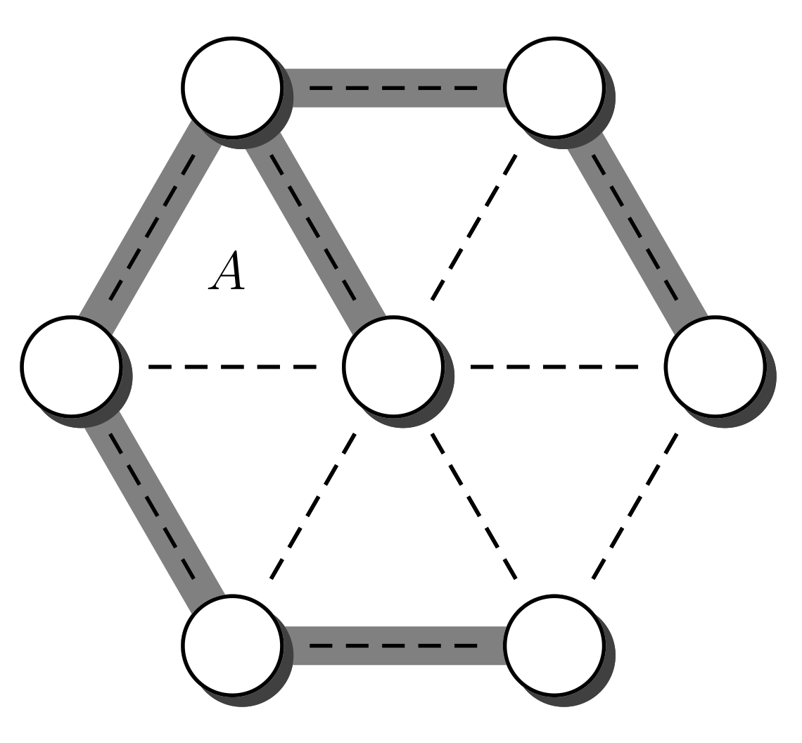
A spanning tree A of an undirected connected graph G is a connected set of edges without cycles that spans every vertex of G. Every vertex of G occurs at an edge of A. Figure 1 shows an example. The vertices of the graph are represented by circles. The set of vertices is denoted by V. The edges of G are represented by dashed lines, and the set of edges is represented by E. The edges of the spanning tree A are represented by thick gray lines. We also use V and E to denote the size of the set V and the size of set E, respectively, i.e., the number of vertices and the number of edges. In case the expression can be interpreted as a set instead of a number, we avoid the ambiguity by writing and , respectively.
We aim to compute one such spanning tree, A, uniformly among all possible spanning trees. The number of these trees may vary significantly, from 1 to , depending on the underlying graph ([1,2,3], Chapter 22). Computing such a tree uniformly and efficiently is challenging for several reasons: the number of such trees is usually exponential; and the structure of the resulting trees is largely heterogeneous as the underlying graphs change. The contributions of this paper are as follows:
- We present a new algorithm, which given a graph G, generates a spanning tree of G uniformly at random. The algorithm uses the link-cut tree data structure to compute randomizing operations in amortized time per operation. Hence, the overall algorithm takes time to obtain a uniform spanning tree of G, where is the mixing time of a Markov chain that is dependent on G. Theorem 1 summarizes this result.
- We propose a coupling to bound the mixing time . The analysis of the coupling yields a bound for cycle graphs (Theorem 2), and for graphs which consist of simple cycles connected by bridges or articulation points (Theorem 3). We also simulate this procedure experimentally to obtain bounds for other graphs. The link-cut tree data structure is also key in this process. Section 4.3 shows experimental results, including other classes of graphs.
This paper is structured as follows. In Section 2 we introduce the problem and explain its subtle nature. In Section 3 we explain our approach and point out that using the link-cut tree data structure is much faster than repeating depth first searches (DFSs). In Section 4 we thoroughly justify our results, proving that the underlying Markov chain has the necessary properties and providing experimental results of our algorithm. In Section 5 we describe the related work concerning random spanning trees, link-cut trees, and mixing times of Markov chains. In Section 6 we present our conclusions.
2. The Challenge
We start by describing an intuitive process for generating spanning trees that does not obtain a uniform distribution. It produces some trees with a higher probability than others. This serves to illustrate that the problem is more difficult than it may seem at first glance. Moreover, we explain why this process is biased, using a counting argument.
A simple procedure to build A consists in using a union-find data structure [4] to guarantee that A does not contain a cycle. Note that these structures are strictly incremental, meaning that they can be used to detect cycles but can not be used to remove an edge from the cycle. Therefore the only possible action is to discard the edge that creates the cycle.
Let us analyze a concrete example of the resulting distribution of spanning trees. We shall show that this distribution is not uniform. First, generate a permutation p of E and then process the edges in this order. Each edge that does not produce a cycle is added to A, edges that would otherwise produce cycles are discarded, and the procedure continues with the next edge in the permutation.
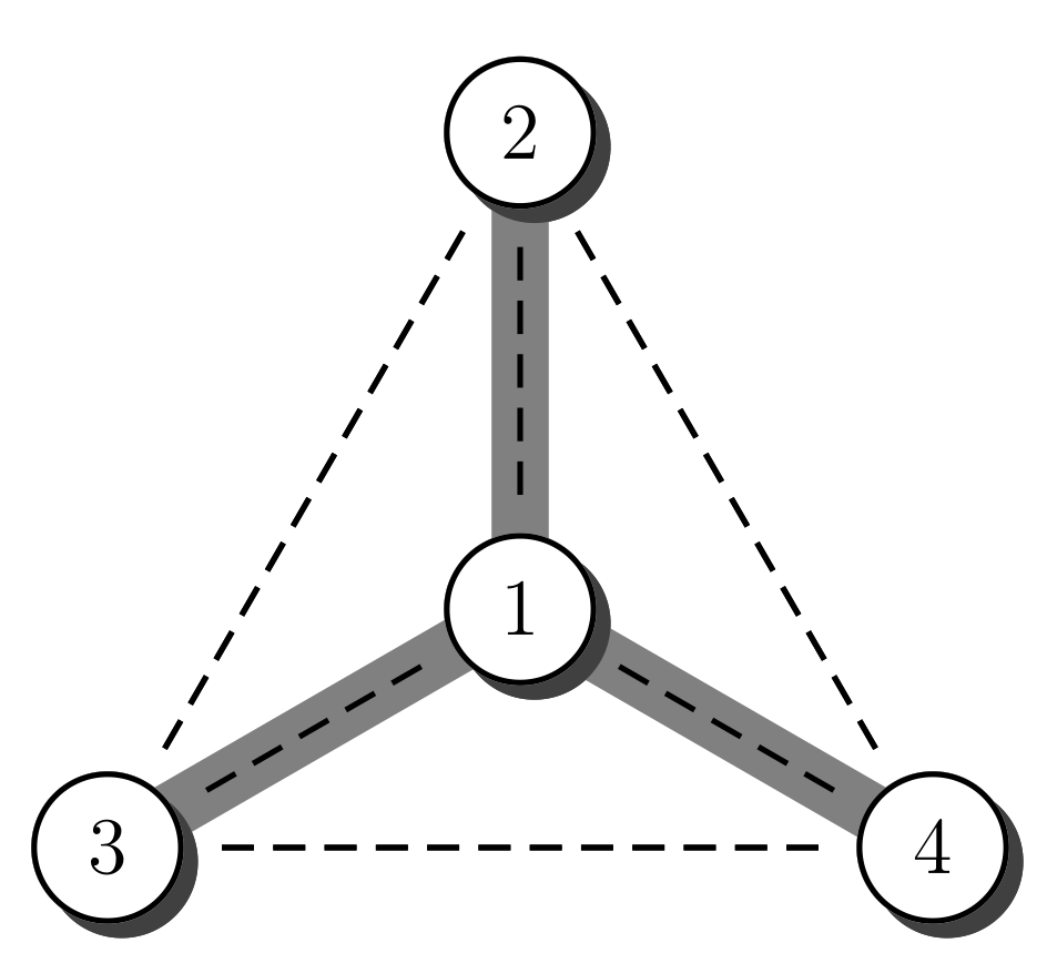
Consider the complete graph on four vertices, , and focus on the probability of generating a star graph, centered at the vertex labeled 1. Figure 2 illustrates the star graph. The graph has 6 edges, hence there are different permutations. To produce the star graph, from one such permutation, it is necessary that the edges and are selected before the edge appears; in general the edges and must occur before . One permutation that generates the star graph is . Now, can be moved to the right to any of three different locations, so we know four sequences that generate the star graph. The same reasoning can be applied to which can be moved once to the right. In total we count 8 different sequences that generate the star graph, centered at 1. For each of these sequences it is possible to permute the vertices , amongst themselves. Hence, we multiply the previous count by . In total we count sequences that generate the star graph, and therefore the total probability of obtaining a star graph is . According to Cayley’s formula, the probability of obtain the star graph centered at 1 should be . Hence, too many sequences generate the star graph centered at 1.
In the next section we fix this bias by discarding some edge in the potential cycle, not necessarily the edge that creates it.
3. Main Idea
To generate a uniform spanning tree, start by generating an arbitrary spanning tree A. One way to obtain this tree is to compute a depth first search in G, in which case the necessary time is . In general, we want the mixing time of our chain to be much smaller than , especially for dense graphs. This initial tree is only generated once, and subsequent trees are obtained by the randomizing process. To randomize A, repeat the next process several times. Choose an edge from E uniformly at random, and consider the set . If already belongs to A the process stops, otherwise contains a cycle C. To complete the process, choose an edge uniformly from and remove it. Hence, at each step the set A is transformed into the set . An illustration of this process is shown in Figure 3.
This edge-swapping process can be adequately modeled by a Markov chain, where the states corresponds to different spanning trees and the transitions among states correspond to the process we have just described. In Section 4.1 we study the ergodic properties of this chain. For now let us focus on which data structures can be used to compute the transition procedure efficiently. A simple solution to this problem would be to compute a depth first search (DFS) on A, starting at u and terminating whenever v is reached. This allows us to identify C in time. Recall that A contains exactly elements. The edge can then be easily removed. Besides G the elements of A also need to be represented with the adjacency list data structure. For our purposes, this approach is inefficient. This computation is central to our algorithm and its complexity becomes a factor in the overall performance. Hence, we will now explain how to perform this operation in only amortized time with the link-cut tree data structure.
The link-cut tree (LCT) is a data structure that can used to represent a forest of rooted trees. The representation is dynamic so that edges can be removed and added. Whenever an edge is removed, the original tree is cut in two. Adding an edge between two trees links them. This structure was proposed by Sleator and Tarjan [5]. Both the link and cut operations can be computed in amortized time.
The LCT can only represent trees; therefore the edge swap procedure must first cut the edge and afterwards insert the edge with the Link operation. The randomizing process needs to identify C and select from it. The LCT can also compute this process in amortized time. The LCT works by partitioning the represented tree into disjoint paths. Each path is stored in an auxiliary data structure, so that any of its edges can be accessed efficiently in amortized time. To compute this process we force the path to become a disjoint path. This means that D will be completely stored in one auxiliary data structure. Hence, it is possible to efficiently select an edge from it. Moreover the size of D can also be computed efficiently. The exact process, to force D into an auxiliary structure, is to make u the root of the represented tree and then access v. Algorithm 1 shows the pseudo-code of the edge-swapping procedure. We can confirm, by inspection, that this process can be computed in the amortized time bound that is crucial for our main result.
| Algorithm 1 Edge-swapping process | |
| 1: procedure EdgeSwap(A) | ▹A is an LCT representation of the current spanning tree |
| 2: Chosen uniformly at random from E | |
| 3: if then | ▹ time |
| 4: | ▹ Makes u the root of A |
| 5: | ▹ Obtains a representation of the path |
| 6: Chosen uniformly from | |
| 7: | ▹ Obtain the i-th edge from D |
| 8: | |
| 9: | |
| 10: end if | |
| 11: end procedure | |
Theorem 1.
If G is a graph and A is a spanning tree of G, then a spanning tree can be chosen uniformly from all spanning trees of G in time, where τ is the mixing time of an ergodic edge-swapping Markov chain.
In Section 4.1 we prove that the process we described is indeed an ergodic Markov chain, thus establishing the result. We finish this section by pointing out a detail in Algorithm 1. In the comment in line 3 we point out that the property must be checked in at most time. This can be achieved in time by keeping an array of Booleans indexed by E. Moreover it can also be achieved in amortized time by using the LCT data structure, essentially by delaying the verification until D is determined and verifying if .
4. The Details
4.1. Ergodic Analysis
In this section, we analyze the Markov chain induced by the edge-swapping process. It should be clear that this process has the Markov property because the probability of reaching a state depends only on the previous state. In other words the next spanning tree depends only on the current tree.
To prove that our procedure is correct we must show that the stationary distribution is uniform for all states. Let us first establish that such a stationary distribution exists. Note that, for a given finite graph G, the number of spanning trees is also finite. More precisely, for complete graphs, Cayley’s formula yields spanning trees. This value is an upper bound for other graphs, as all spanning trees of a certain graph are also spanning trees of the complete graph with the same number of vertices. Therefore, the chain is finite. If we show that it is irreducible and aperiodic, it follows that it is ergodic ([6], Corollary 7.6) and therefore it has a stationary distribution ([6], Theorem 7.7).
The chain is aperiodic because self-loops may occur, i.e., transitions where the underlying state does not change. Such transitions occur when is already in A, and therefore their probability is at least , because there are edges in a spanning tree A.
To establish that the chain is irreducible it is sufficient to show that for any pair of states i and j there is a non-zero probability path from i to j. First note that the probability of any transition on the chain is at least , because is chosen out of E elements and is chosen from , that contains at most edges. To obtain a path from i to j let and represent the respective trees. We consider the following cases:
- If we use a self-loop transition.
- Otherwise, when , it is possible to choose from , and from ; note that the set equality follows from the assumption that belongs to . For the last property, note that if no such exists then , which is a contradiction because is a tree and C is a cycle. As mentioned above, the probability of this transition is at least . After this step the resulting tree is not necessarily , but it is closer to that tree. More precisely is not necessarily , however the set is smaller than the original . Its size decreases by 1 because the edge exists on the second set but not on the first. Therefore, this process can be iterated until the resulting set is empty and therefore the resulting tree coincides with . The maximal size of is , because the size of is at most . This value occurs when and do not share edges. Multiplying all the probabilities in the process of transforming into we obtain a total probability of at least .
Now that the stationary distribution is guaranteed to exist, we will show that it coincides with the uniform distribution by proving that the chain is time-reversible ([6], Theorem 7.10). We prove that for any pair of states i and j, with , for which there exists a transition from i to j, with probability , there exists, necessarily, a transition from j to i with probability . If the transition from i to j exists it means that there are edges and such that , where belongs to the cycle C contained in . Hence, we also have that , which means that the tree can be obtained from the tree by adding the edge and removing the edge . In other words, the process in Figure 3 is similar both top down or bottom up. This process is a valid transition in the edge-swap chain, where the cycle C is the same in both transitions, i.e., C is the cycle contained in and in . Now we obtain our result by observing that . In the transition from i to j, the factor comes from the choice of and the factor from the choice of . In the transition between j to i, the factor comes from the choice of and the factor from the choice of . Hence, we established that the algorithm we propose correctly generates spanning trees uniformly, provided we can sample from the stationary distribution. Hence, we need to determine the mixing time of the chain, i.e., the number of edge swap operations that need to be performed on an initial tree until the distribution of the resulting trees is close enough to the stationary distribution.
Before analyzing the mixing time of this chain we point out that it is possible to use a faster version of this chain by choosing uniformly from , instead of from E. This makes the chain faster, but proving that it is aperiodic is trickier. In this chain we have that , for any state i. We will now prove that , for any state i and . It is enough to show for and , all other values follow from the fact that the greatest common divisor of 2 and 3 is 1. For the case of we use the time reverse property and the following deduction: . For the case of we observe that the cycle C must contain at least three edges , and . To obtain we insert and remove ; now we move from this state to state by inserting and removing . Finally we move back to by inserting and removing . Hence, for this case we have .
4.2. Coupling
In this section, we focus on bounding the mixing time. We did not obtain general analytical bounds from existing analysis techniques, such as couplings [6,7], strong stopping times [7] and canonical paths [8]. The coupling technique yielded a bound only for cycle graphs and moreover a simulation of the resulting coupling converges for ladder graphs.
Before diving into the reasoning in this section, we first need a finer understanding of the cycles generated in our process. We consider a closed walk to be a sequence of vertices , starting and ending at the same vertex, such that any two consecutive vertices and are adjacent; in our case . The cycles we consider are simple in the sense that they consist of a set of edges for which a closed walk can be formed that traverses all the edges in the cycle, and moreover no vertex repetitions are allowed, except for the vertex , which is only repeated at the end. Formally this can be stated as: if and , then .
The cycles that occur in our randomizing process are even more regular. A cordless cycle in a graph is a cycle such that no two vertexes of the cycle are connected by an edge that does not itself belong to the cycle. The cycles we produce also have this property, otherwise if such a chord existed then it would form a cycle on our tree A, which is a contradiction. In fact, a spanning tree over a graph can alternatively be defined as a set of edges such that for any pair of vertices v and there is exactly one path linking v to .
A coupling is an association between two copies of the same Markov chain and , in our case the edge-swapping chain. The goal of a coupling is to make the two chains meet as fast as possible, i.e., to obtain , for a small value of . At this point we say that the chains have coalesced. The two chains may share information and cooperate towards this goal. However, when analyzed in isolation, each chain must be indistinguishable from the original chain . Obtaining with a high probability implies that at time the chain is well mixed. Precise statements of these claims are given in Section 5.
We use the random variable to represent the state of the first chain, at time t. The variable represents the state of the second chain. We consider the chain in state x and the chain in state y. In one step, the chain will transition to the state and the chain will transition to state .
The set contains the edges that are exclusive to and likewise the set contains the edges that are exclusive to . The number of such edges provides a distance that measures how far apart the two states are. We refer to this distance as the edge distance. We define a coupling when , which can be extended for states x and y that are farther apart by using the path-coupling technique [9].
To use the path-coupling technique we cannot alter the behavior of the chain as, in general, it is determined by the previous element in the path. We denote by the edge that gets added to , and by the edge that gets removed from the corresponding cycle , in the case such a cycle exists. Likewise, represents the edge that is inserted into and the edge that gets removed from the corresponding cycle , in the case such a cycle exists. The edge is chosen uniformly at random from E and is chosen uniformly at random from . The edges and will be obtained by trying to mimic the chain , but still exhibiting the same behavior as . In this sense the information flows from to . Let us now analyze .
4.2.1.
If then , which means that the corresponding trees are also equal, . In this case uses the same transition as , by inserting , i.e., set , and by removing , i.e., set .
4.2.2.
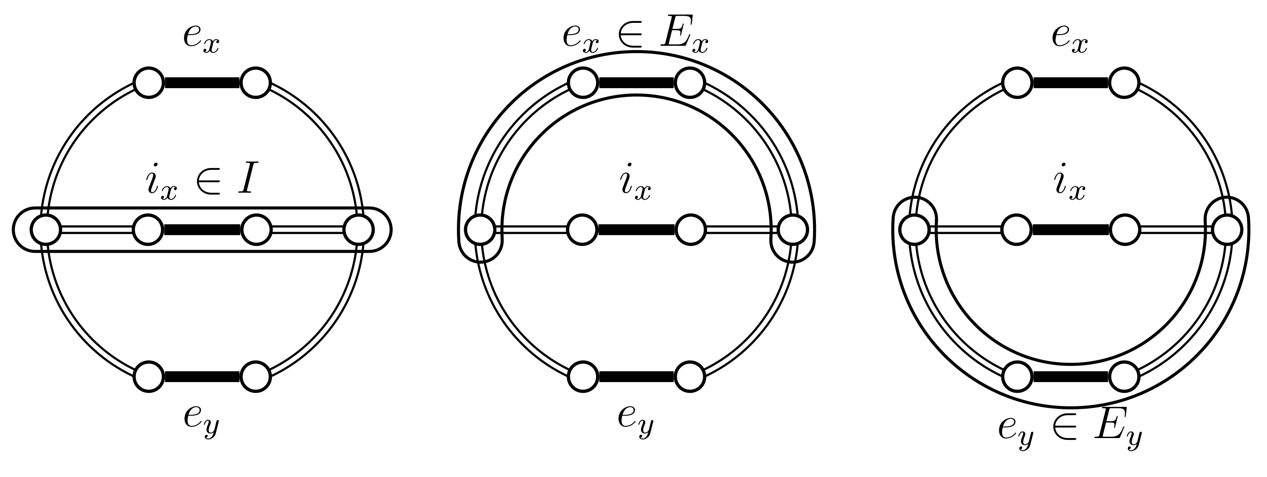
If then the edges and exist and are distinct. We also need the following sets: , and . The set I represents the edges that are common to and . The set represents the edges that are exclusive to , from the cycle point of view. This should not be confused with which represents the edge that is exclusive to , i.e., from a tree point of view. Likewise, represents the edges that are exclusive to . Also we consider the cycle as the cycle contained in , which necessarily contains . The following Lemma describes the precise structure of these sets.
Lemma 1.
When we either have and therefore , or , and I form simple paths, and the following properties hold:
- , ,
- , ,
- , , .
Notice that in particular this means that, in the non-trivial case, and partition . A schematic representation of this Lemma is shown in Figure 4.
We have several different cases described below. Aside from the lucky cases 2 and 3, we will usually choose , as tries to copy . Likewise, if possible, we would like to set . When this is not possible we must choose , ideally we would choose , but we must be extra careful with this process to avoid losing the behavior of . To maintain this behaviour, we must sometimes choose . Since provides no information on this type of edges, we use chosen uniformly from this , i.e., select from but not nor edges that are also in .
There is a final twist to this choice, which makes the coupling non-Markovian, i.e., it does not verify the conditions in Equations (1a) and (1b). We can choose more often than would otherwise be permissible by keeping track of how was determined. If is obtained deterministically, for example by the initial selection of x and y, then this is not possible. In general might be determined by the changes in , in which case we want to take advantage of the underlying randomness. Therefore, we keep track of the random processes that occur. The exact information we store is a set of edges , such that , and moreover this set contains the edges that are equally likely to be . This information can be used to set when , however after such an action the information on must be purged.
To illustrate the possible cases we use Figure 5, Figure 6, Figure 7, Figure 8, Figure 9, Figure 10, Figure 11, Figure 12, Figure 13, Figure 14 and Figure 15, where the edges drawn with double lines represent a generic path that may contain several edges, or none at all. The precise cases are as follows:
- If the chain loops (), because , then also loops and therefore . The set does not change, i.e., set .
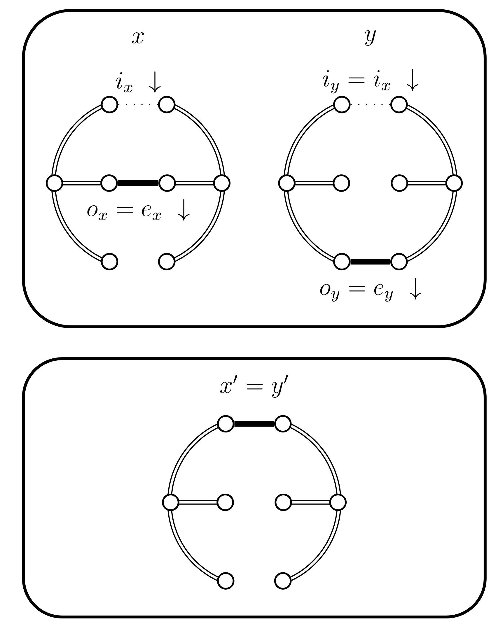
- If and then set and . In this case the chains do not coalesce; they swap states because and (see Figure 5). Set .
- If and then set and . In this case the chains coalesce, i.e., (see Figure 6). When the chains coalesce, the edges and no longer exist and the set is no longer relevant.
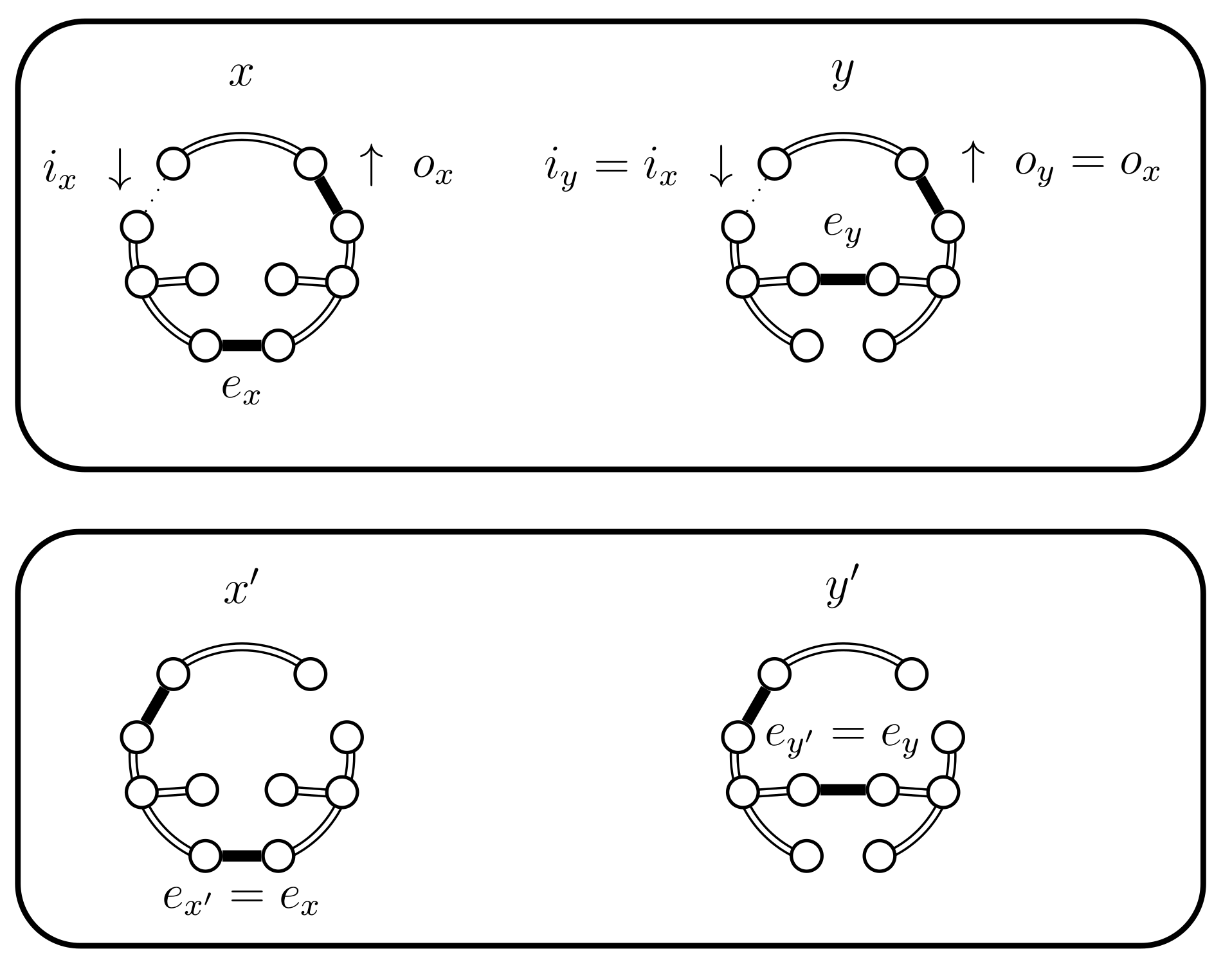
- If set . We now have three sub-cases, which are further sub-divided. These cases depend on whether , or . We start with which is simpler and establishes the basic situations. When or we use some Bernoulli random variables to balance out probabilities and whenever possible reduce to the cases considered for . When this is not possible we present the corresponding new situation.
- (a)
- If we have the following situations:
- (i)
- If then set . In this case the chains coalesce (see Figure 7).
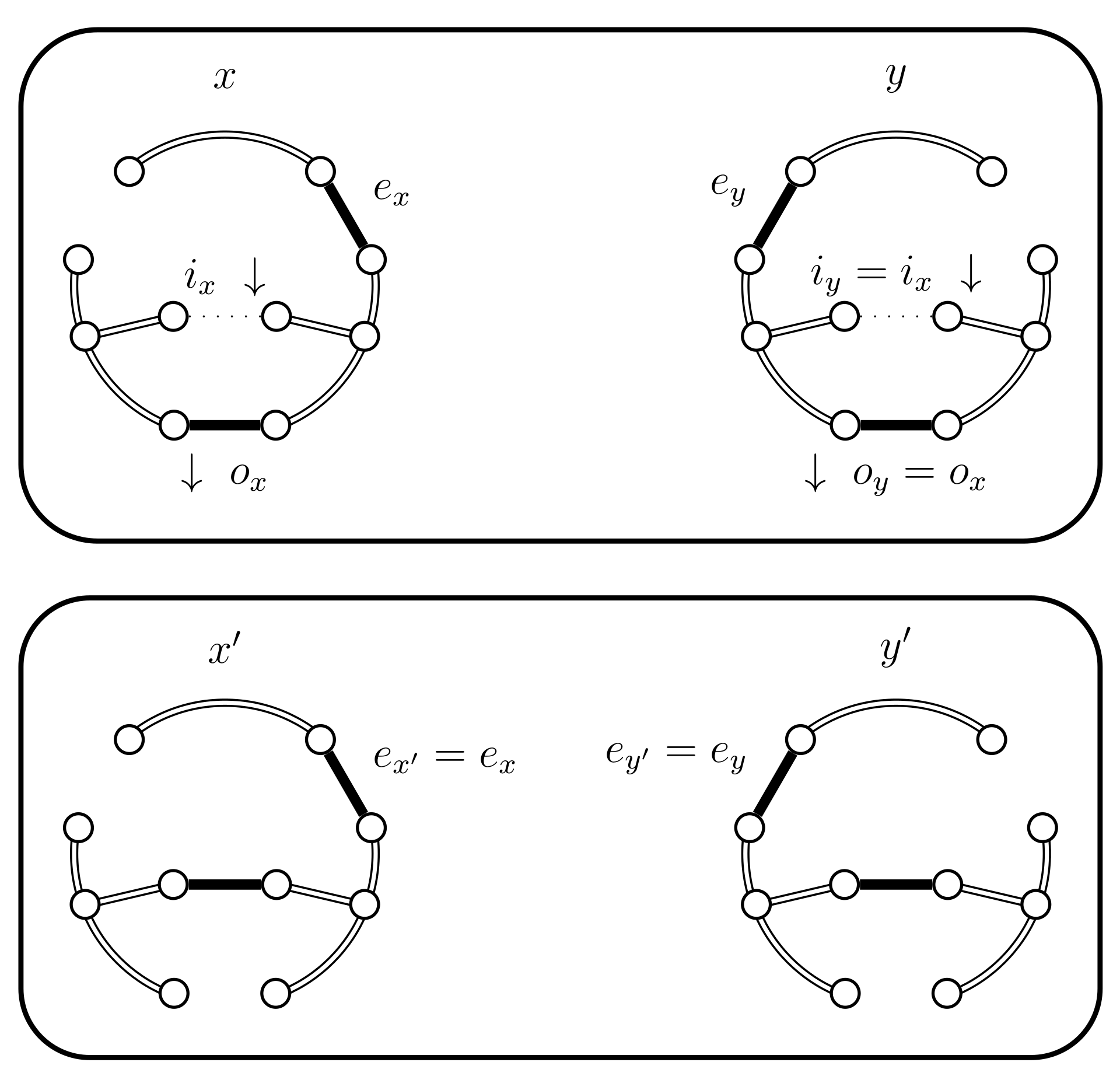
- (ii)
- (iii)
- If then select uniformly from . If then set (see Figure 10). In this case set . The alternative, when , is considered in the next case (4.a.iv).
- (iv)
- If and , then set . This case is shown in Figure 11. In this case the distance of the coupled states increases, i.e., . Therefore we include a new state in between and and define to be the edge in ; the edge in ; and the edge in . The set should contain the edges that provide alternatives to . In this case set and .
- (b)
- If then will choose with a higher probability then what should. Therefore, we use a Bernoulli random variable B with a success probability p defined as follows:In Lemma 2 we prove that p properly balances the necessary probabilities. For now note that when the expression for p yields . This is coherent with the following cases, because when B yields true we use the choices defined for . The following situations are possible:
- (i)
- (ii)
- (iii)
- If and B fails and . We have a new situation,;set . The distance increases, (see Figure 14). Set and .
- (iv)
- (c)
- If we have the following situations:
- (i)
- If then use case 4.a.i and set (see Figure 7). The chains coalesce.
- (ii)
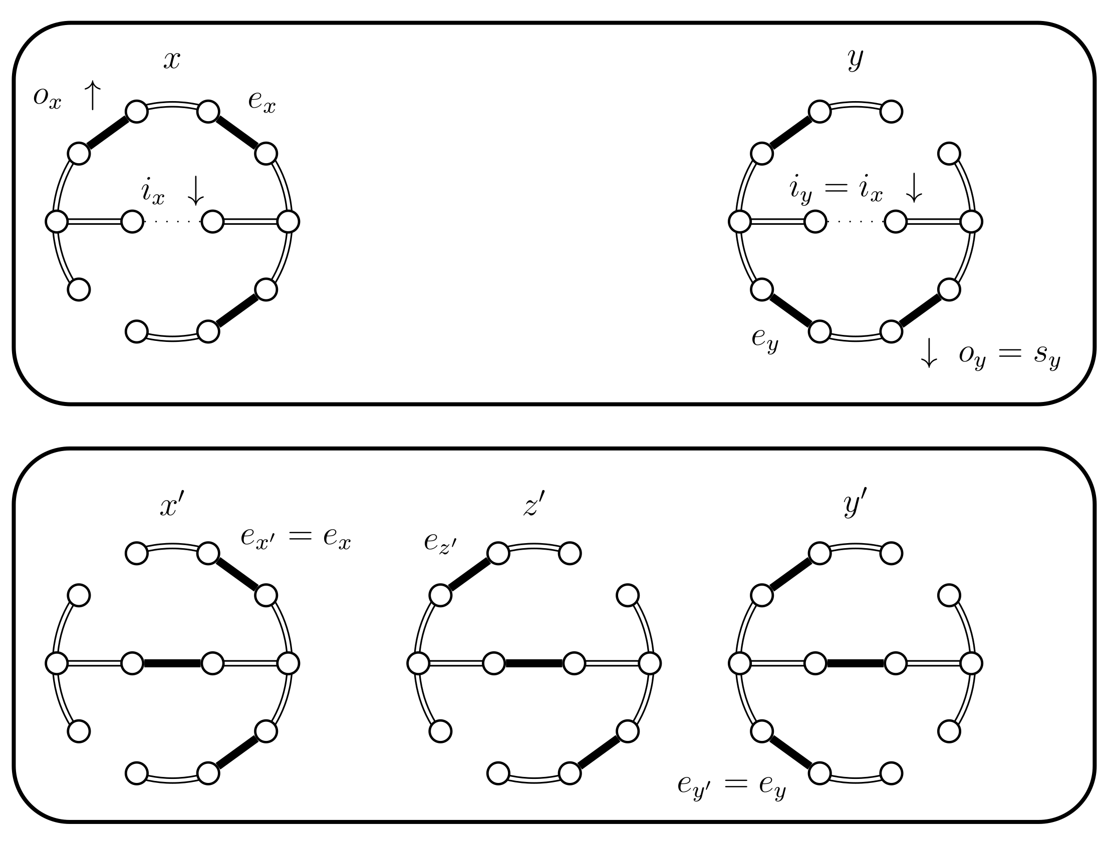
- (iii)
- If then we use a new Bernoulli random variable with a success probability defined as follows:In Lemma 2 we prove that properly balances the necessary probabilities. For now, note that when the expression for yields , because becomes 0. This is coherent because when returns false we will use the choices defined for . The case when fails is considered in the next case (4.c.iv).If is successful we have a new situation. Set , where is chosen uniformly from (see Figure 15). We have , , and .
- (iv)
- If and fails we use another Bernoulli random variable with a success probability defined as follows:
Notice that the case 4.a.ii applies when , thus solving this situation as a particular case. This case is shown in Figure 8. It may even be the case that and and are disjointed, i.e., . This case is not drawn.
Formally, a coupling is Markovian when Equations (1a) and (1b) hold, where is the coupling, which is defined as a pair of chains . The chain represents the original chain.
To establish vital insight into the coupling structure we will start by studying it when it is Markovian.
Lemma 2.
When , the process we described is a Markovian coupling.
Proof.
The coupling verifies Equation (1a), because we do not alter the behavior of the chain . Hence the main part of the proof focuses on Equation (1b).
First, let us prove that for any edge the probability that is , i.e., . The possibilities for are the following:
- : this occurs only in case 1, when . It may be that ; this occurs when , in which case and this is the only case where . In this case . Otherwise, , in these cases , and therefore .
- : this occurs in cases 2 and 3, i.e., when , which is the decisive condition for this choice. Therefore .
- : this occurs in case 4. In this case so again we have that .
Before focusing on we will prove that the Bernoulli random variables are well defined, i.e., that the expressions on the denominators are not 0 and that the values of p, , are between 0 and 1.
- Analysis of B. We need to have for p to be well defined. Any cycle must contain at least three edges; therefore and hence . This guarantees that the denominator is not 0. The same argument proves that , thus implying that , as both expressions are positive. We also establish that because of the hypothesis of case 4.b which guarantees and therefore .
- Analysis of . As in seen the analysis of B we have that and , therefore those denominators are not 0. Moreover we also need to prove that . In general we have that , because . Moreover, the hypothesis of case 4.c.iii is that and therefore , which is obtained by removing I from the both sides. This implies that and therefore , thus establishing that the last denominator is also not 0.Let us now establish that and . Note that can be simplified to the expression , where all the expressions in parenthesis are non-negative, so . For the second property we use the new expression for and simplify to . The deduction is straightforward using the equality that is obtained by removing I from the left side. The properties and establish the desired result.
- Analysis of . We established, in the analysis of B, that is non-zero. In the analysis of we also established that is non-zero. Note that case 4.c.iv also assumes the hypothesis that . Moreover, in the analysis of we also established that , which implies that and therefore the last denominator is also non-zero.Let us also establish that and . For the second property we instead prove that , where and all of the expressions in parenthesis are non-negative. We use the following deduction of equivalent inequalities to establish that :This last inequality is part of the hypothesis of case 4.c.iv.
Now, let us focus on the edge . We wish to establish that for any we have that . We analyze this edge according to the following cases:
- When the cycles are equal . This involves cases 2 and 3.
- : this occurs only in case 2 and it is determined by the fact that . Therefore, .
- : this occurs only in case 3 and it is determined by the fact that , in this case . Therefore .
- When the cycles have the same size (case 4.a). The possibilities for o are as follows:
- : this occurs only in the case 4.a.i. This case is determined by the fact that . Therefore, . Note that according to the Lemma’s hypothesis, case 4.a.iii never occurs.
- : this occurs only in case 4.a.ii. This case is determined by the fact that and sets . Therefore, .
- : this occurs only in case 4.a.iv. This case is determined by the fact that and moreover sets , which was uniformly selected from . We have the following deduction where we use the fact that the events are independent and that implies :
- When this involves case 4.b. The cases for o are as follows:
- : this occurs only in the case 4.b.i and when B is true. This case occurs when . We make the following deduction, that uses the fact that the events are independent and the success probability of B:
- : this occurs only in case 4.b.ii and when B is true. This case is determined by the fact that and sets . We make the following deduction, that uses the fact that the events are independent and the success probability of B:
- : this occurs in case 4.b.iv, but also in cases 4.b.iii and 4.b.i when B is false. We have the following deduction, that uses event independence, the fact that the cases are disjoint events, and the success probability of B:
- When , this concerns case 4.c. The cases for o are the following:
- : this occurs in the case 4.c.i and case 4.c.iv when is true. We use the following deduction:
- : this occurs in case 4.c.ii and case 4.c.iii when is true. We make the following deduction:
- : this occurs in case 4.c.iv when is false. We have the following deduction:
☐
Lemma 3.
The process we described is a non-Markovian coupling.
Proof.
In the context of a Markovian coupling we analyze the transition from y to given the information about x. In the non-Markovian case we will use less information about x. We assume that is a random variable and that x provides only and ; we know only that and moreover that for any and otherwise. Then the chain makes its move and provides information about and . Let us consider only the cases when and choose , because nothing changes in the cases where this does not happen. Now, can be used to define and and, therefore, and . We focus our attention on because, except for the trivial cases, we must have . Hence, we instead alter our condition to , for any and 0 otherwise.
Note that this is a reasonable process because we established in Lemma 1 that, in the non-trivial case, and partition and, therefore, because , we have that and also partition . This means that and so we are not losing any part of in this process; we are only dividing it into cases. This process is also the reason why, even when , we define .
Now the cases considered in Lemma 2 must be changed. Substitute the original cases of for . Also, substitute the case for . The other cases remain unaltered. Except for the first case, the previous deductions still apply. We will exemplify how the deduction changes for . We consider only the situation when . For the remaining situations, and , we use a general argument. Hence our precise assumptions are: and .
This is correct according to our assumption.
The general argument follows the above derivation. Whenever the Markovian coupling produces , we obtain a probability of. Moreover, for every edge produced by the Markovian coupling such that , we obtain another probability. This totals , as desired. This also occurs in the cases when and , only the derivations become more cumbersome.
Finally will argue why when . The set is initialized to contain only the edge , i.e., . As the coupling proceeds, is chosen to represent the edges, from which was chosen, or is simply restricted if does not change. More precisely, in case 4.a.iii we choose ; in case 4.b.iv we choose ; and in case 4.b.ii we choose . ☐
We obtained no general bounds on the coupling we presented; it may even be that such bounds are exponential even if the Markov chain has a polynomial mixing time. In fact, Kumar and Ramesh [10] proved that this is the case for Markovian couplings of the Jerrum–Sinclair chain [11]. Note that according to the classification of Kumar and Ramesh [10] the coupling we present is considered as time-variant Markovian. Hence their result applies to the type of coupling we are using, although we are considering different chains so it is not immediately seen that indeed there exist no polynomial Markovian couplings for the chain we presented. Cycle graphs are the only class of graphs for which we establish polynomial bounds (see Figure 16).
Theorem 2.
For any cycle graph G the mixing time τ of edge-swap chain is for the normal version of the chain and for the fast version.
Proof.
For any two trees and we have a maximum distance of one edge, i.e., . Hence our coupling applies directly.
For the fast version, case 1 does not occur, because is chosen from . Hence, the only cases that might apply are cases 2 and 3. In first case, the chains preserve their distance and in the last case the distance is reduced to 0. Hence, , which corresponds to the probability of case 2. Each step of the coupling is independent, which means we can use the previous result and Markov’s inequality to obtain . Then, we use this probability in the coupling Lemma 4 to obtain a variation distance of , by solving the following equation: .
For the slow version of the chain, case 1 applies most of the time, i.e., for out of V choices of . It takes steps for the standard chain to behave as the fast chain and, therefore, the time should be . ☐
This result is in stark contrast with the alternative methods, the random walk and Wilson’s (see Section 5) algorithms, which require time [7]. More recent algorithms are also at least for this case.
Moreover when a graph is a connected set of cycles linked by bridges or articulation points we can also establish a similar result. Figure 17 shows one such graph.
Theorem 3.
For any graph G which consists of n simple cycles connected by bridges or articulation points, such that m is the size of the smallest cycle, then the mixing time τ of the fast edge swap chain is as follows:
The mixing time for the slow version is obtained by using instead of n in the previous expression.
Proof.
To obtain this result we use a path-coupling argument. Then, for two chains at distance 1 we have .
We assume that the different edge occurs in the largest cycle. In general the edges inserted and deleted do not alter this situation, hence the term 1. However with probability the chain inserts an edge that creates the cycle where the difference occurs. In that case with probability the chains coalesce. Hence applying path-coupling the mixing time must verify the following equation:
For the slow version the chain choose the correct edge with probability instead of . ☐
4.3. Experimental Results
4.3.1. Convergence Testing
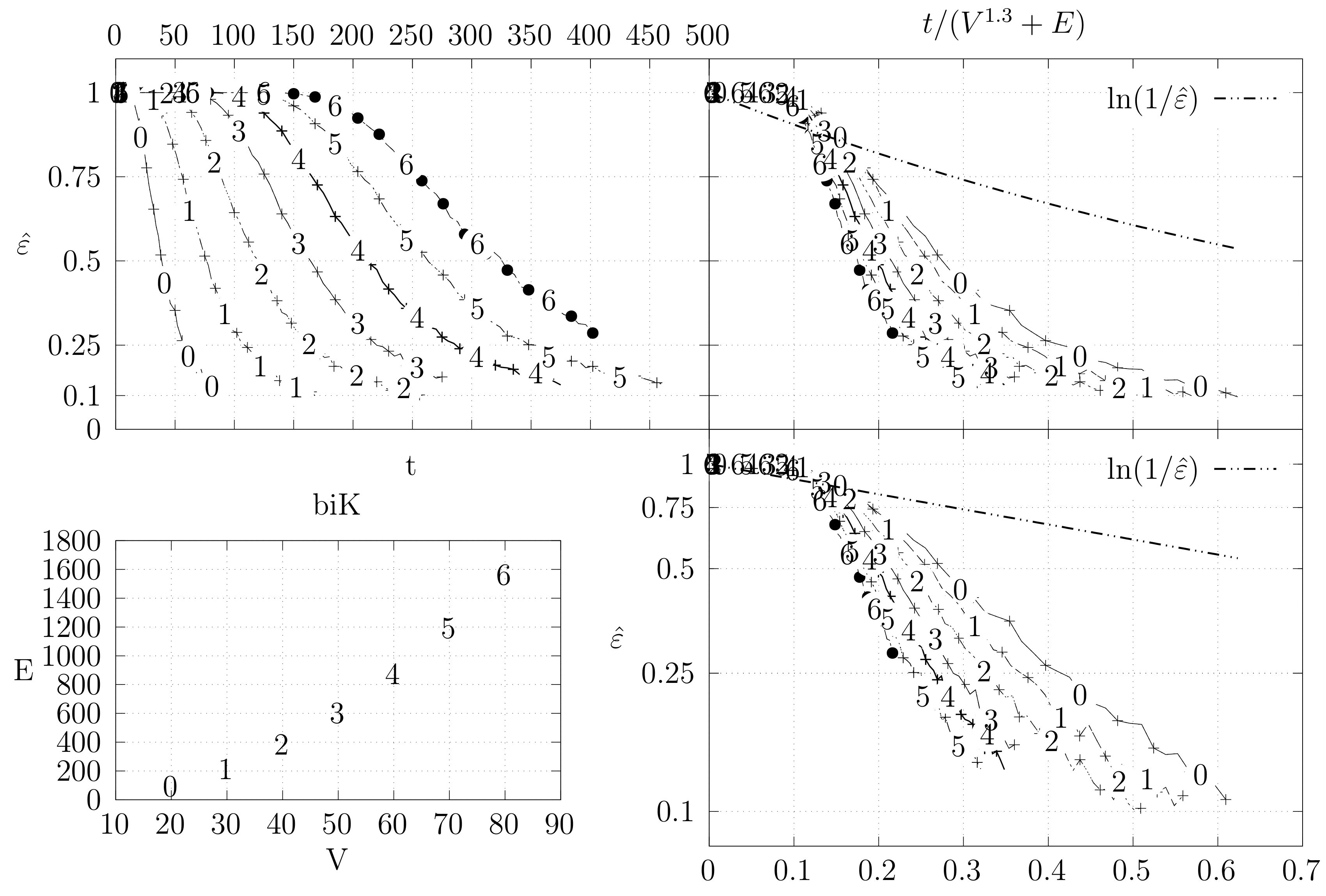
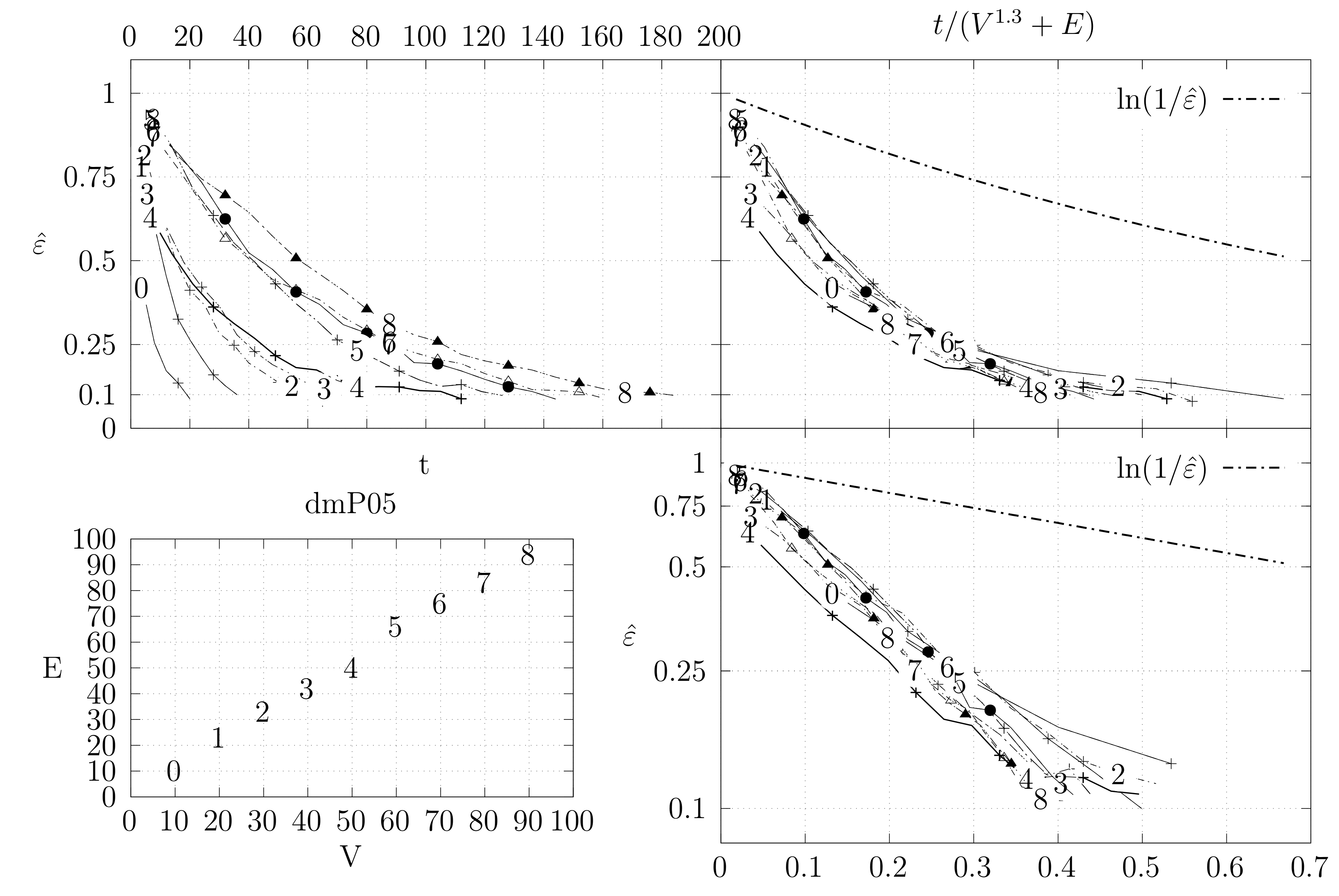
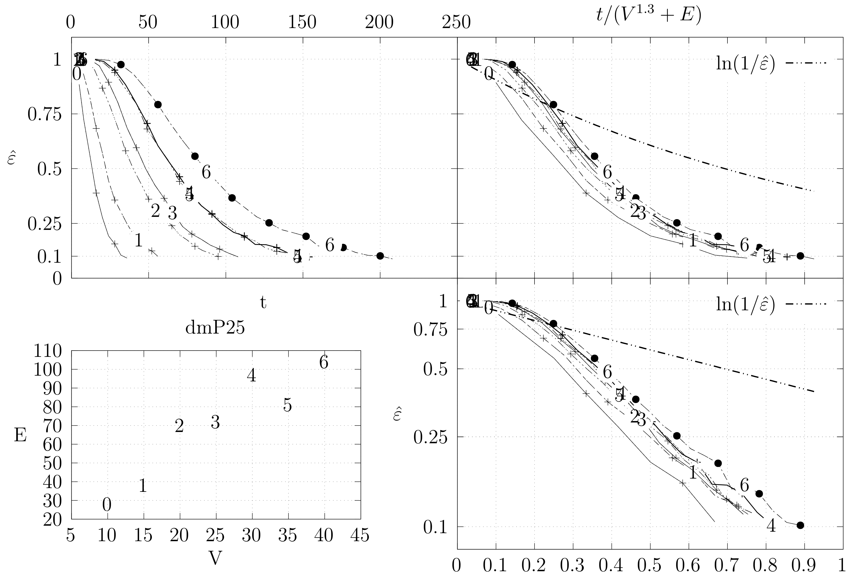
Before looking at the performance of the algorithm we started by testing the convergence of the edge swap chain. We estimate the variation distance after a varying number of iterations. The results are shown in Figure 18, Figure 19, Figure 20, Figure 21, Figure 22, Figure 23 and Figure 24. We now describe the structure of these figures. Consider for example Figure 20. The structure is as follows:
- The bottom left plot shows the graph properties, the number of vertices V in the x axis and the number edges E on the y axis. For the dense case graph 0 has 10 vertices and 45 edges. Moreover, graph 6 has 40 vertices and 780 edges. These graph indexes are used in the remaining plots.
- The top left plot shows the number of iterations t of the chain in the x axis and the estimated variation distance on the y axis, for all the different graphs.
- The top right plot is similar to the top left, but the x axis contains the number of iterations divided by . Besides the data this plot also shows a plot of for reference.
- The bottom right plot is the same as the top right plot, using a logarithmic scale on the y axis.
To avoid the plots from becoming excessively dense, we do not plot points for all experimental values, instead we plot one point out of three. However, the lines pass through all experimental points, even those that are not explicit.
The different values at the end of dmP, namely in Figure 22, Figure 23 and Figure 24, correspond to the choices of p.
The variation distance between two distributions and on a countable state space S is given by . This is the real value of . However, the size of S quickly becomes larger than we can compute. Instead, we compute a simpler variation distance , where S is reduced from the set of all spanning trees of G to the set of integers from 0 to , which correspond to the edge distance, defined in Section 4.2, of the generated tree A to a fixed random spanning tree R. More precisely, we generate 20 random trees, using a random walk algorithm described in Section 5. For each of these trees, we compute , i.e., the simpler distance between the stationary distribution and the distribution obtained by computing t steps of the edge-swapping chain. To obtain , we start from a fixed initial tree and execute our chain t times. This process is repeated several times to obtain estimates for the corresponding probabilities. We keep two sets of estimates and and stop when . Moreover, we only estimate values where . We use the same criteria to estimate , but in this case the trees are again generated by the random walk algorithm. The final value is obtained as the maximum value obtained for the 20 trees.
We generated dense graphs, cycle graphs, sparse graphs, and some in-between graphs. The cycle graphs consist of a single cycle, as shown in Figure 16.The sparse graphs are ladder graphs; an illustration of these graphs is shown in Figure 25.
The dense graphs are actually the complete graphs . We also generated other dense graphs labeled biK which consisted of two complete graphs connected by two edges. Graphs were also generated based on the duplication model dmP. Let be an undirected and unweighted graph. Given , the partial duplication model builds a graph by partial duplication as follows [12]: start with at time and, at time , perform a duplication step:
- Uniformly select a random vertex u of G.
- Add a new vertex v and an edge .
- For each neighbor w of u, add an edge with probability p.
These graphs show the convergence of the Markov chain and moreover seems to be a reasonable bound for . Still, these results are not entirely binding. On the one hand the estimation of the variation distance groups several spanning trees into the same distance, which means that within a group the distribution might not be uniform, even if the global statistics are good. Hence, the actual variation distance may be larger and the convergence might be slower. On the other hand, we chose the exponent 1.3 experimentally by trying to force the data of the graphs to converge at the same point. The actual value may be smaller or larger.
4.3.2. Coupling Simulation
As mentioned before, we obtained no general bounds on the coupling we presented. In fact, experimental simulation for the coupling does not converge for all classes of graphs. We obtained experimental convergence for cycle graph, as expected from Theorem 2, and for ladder graphs. For the remaining graphs we used an optimistic version of the coupling which always assumes that and that fails. With these assumptions, all the cases which increase the distance between states are eliminated and the coupling always converges. Note that this approach does not yield sound coupling, but in practice we verified that this procedure obtained good experimental variation distance. Moreover, the variation distance estimation for these tests is not the simpler distance but the actual experimental variation distance, obtained by generating several experimental trees, such that in average each possible tree is obtained 100 times.
The simulation of the path coupling proceeds by generating a path with steps, essentially selecting two trees at distance from each other. This path is obtained by computing steps of the fast chain. Recall that our implementation and all simulations use the fast version of the chain. The simulation ends once this path contracts to size . Let be the number of steps in this process. Once this point is obtained, our estimate for mixing time is . In general, we wish to obtain such that the probability that the two general chains and coalesce is at least . Hence, we repeat this process four times and choose the second largest value of as our estimate.
Table 1 summarizes results for the experimental variation distance. The number of possible spanning trees for each graph was computed with Kirchhoff’s theorem. Then, we generated 100 times the number of possible trees, and we computed the variation distance. As stated above, we obtained good results for the variation distance, getting a median well below 25% for all tested graph topologies.
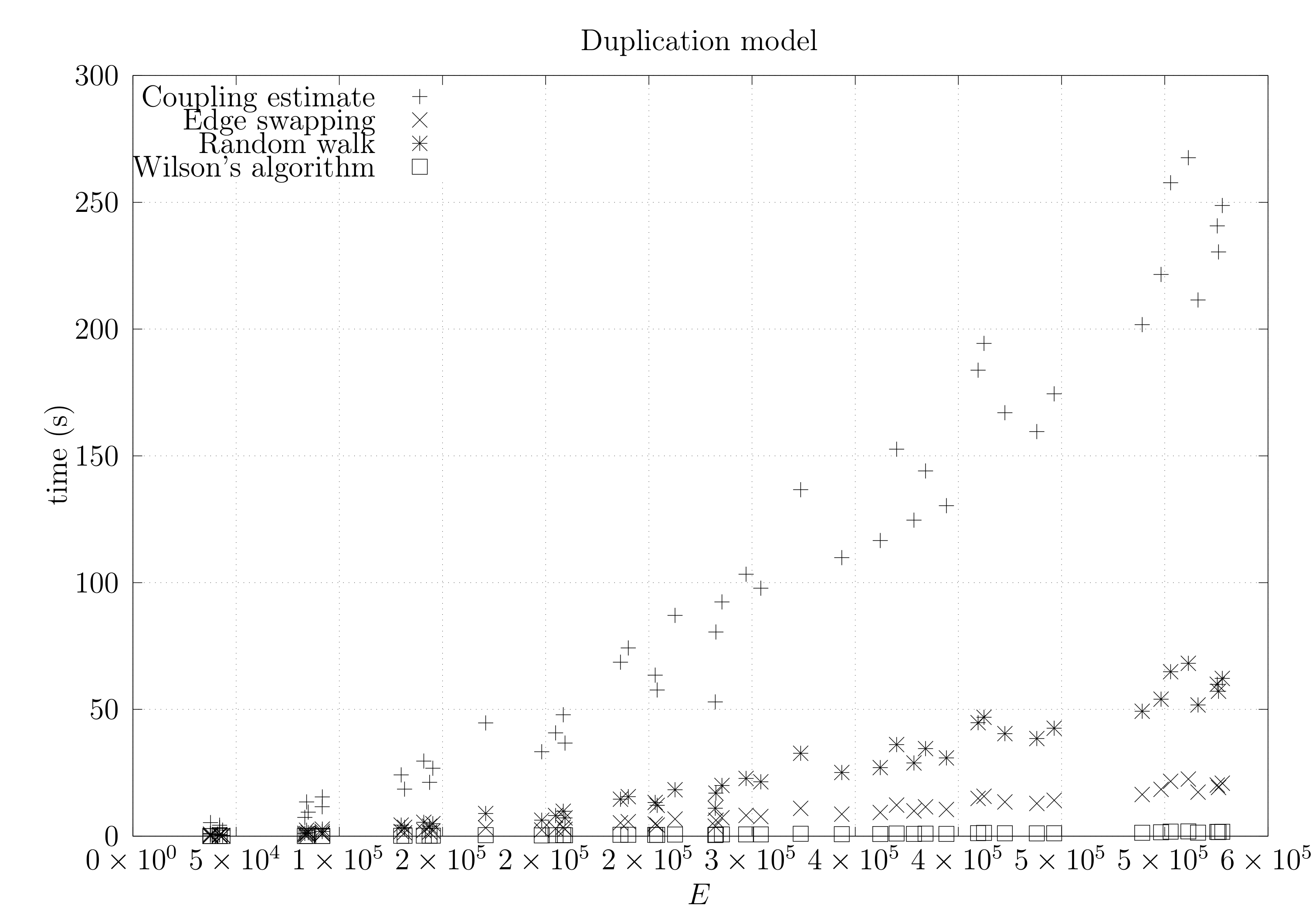
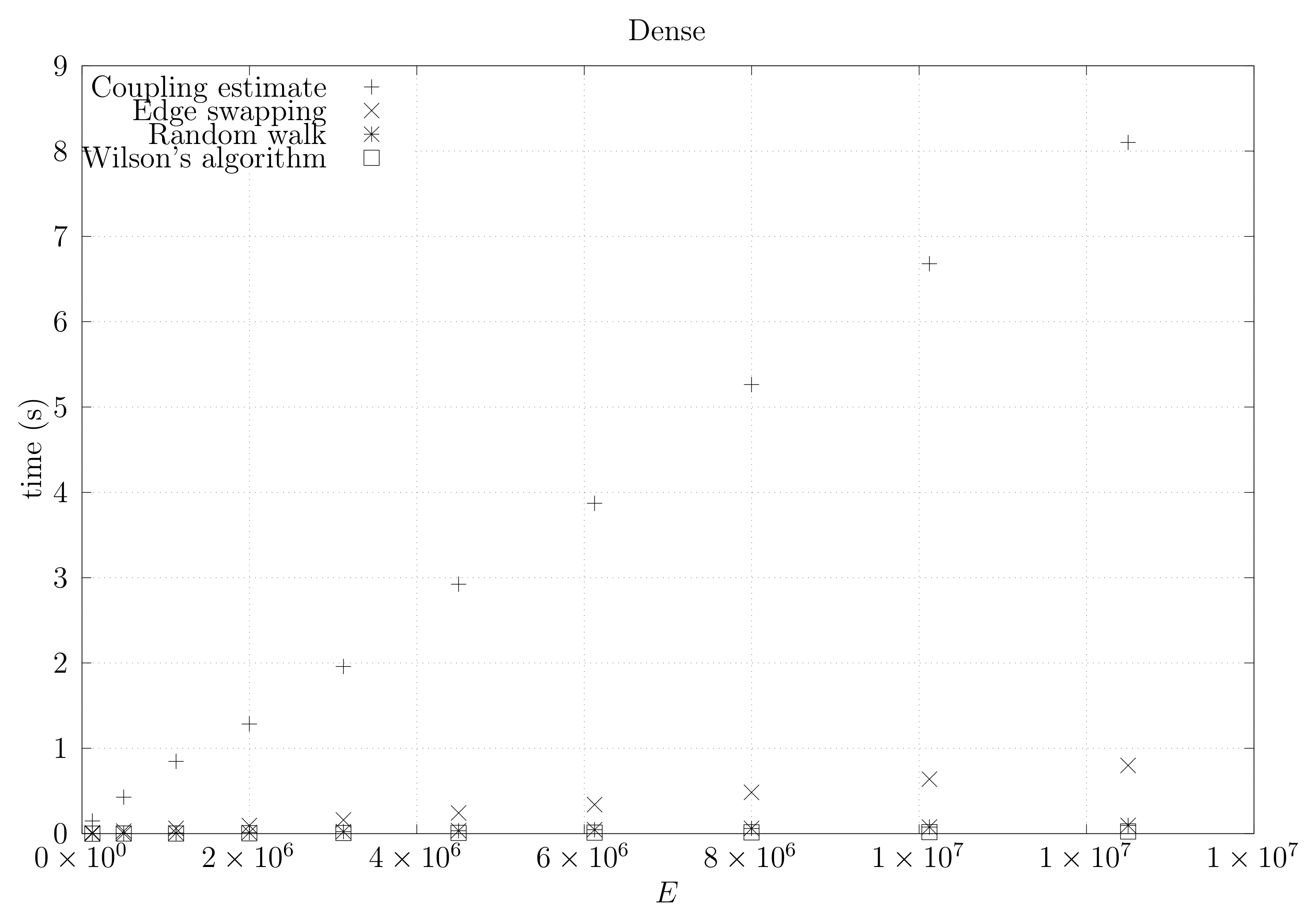
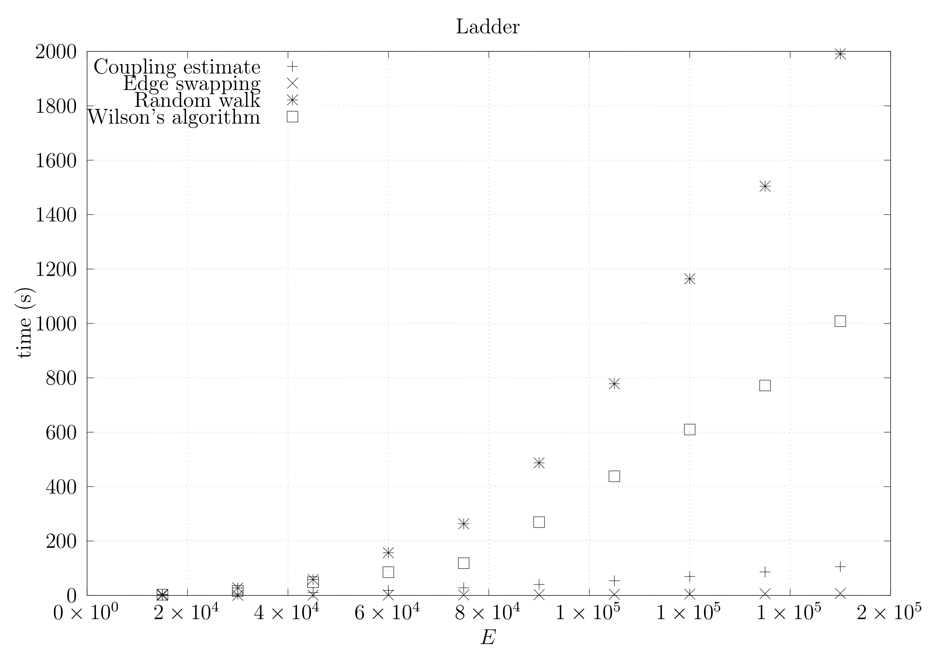
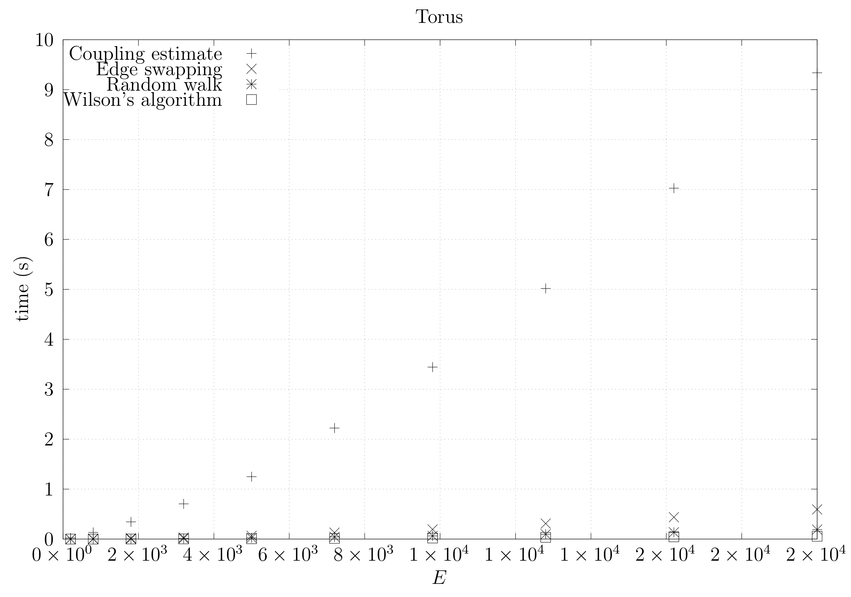
We now present experimental results for larger graphs where we use the optimistic coupling. All experiments were conducted on a computer with an Intel(R) Xeon(R) CPU E5-2630 v3 @ 2.40 GHz with 4 cores and 32 GB of RAM. We present running times for different graph topologies and sizes in Figure 26, Figure 27, Figure 28, Figure 29, Figure 30, Figure 31 and Figure 32. Note beforehand that the coupling estimate needs only to be computed once for each graph. Once the estimate is known, we can generate as many spanning trees as we want. Although the edge-swapping method is not always the faster compared with the random walk and Wilson’s algorithms, it is competitive in practice for dmP and torus graphs, and it is faster for biK, cycle and sparse (ladder) graphs. As expected, it is less competitive for dense graphs. Hence, experimental results seem to point out that the edge-swapping method is more competitive in practice for those instances that are harder for random walk-based methods, namely biK and cycle graphs. The results for biK and dmP are of particular interest as most real networks seem to include these kind of topologies, i.e., they include communities and they are scale-free [13].
5. Related Work
For detailed information on probabilities for trees and networks, see Lyons and Peres [14] (Chapter 4). As far as we know, the initial work on generating uniform spanning trees was performed by Aldous [15] and Broader [16], who obtained spanning trees by performing a random walk on the underlying graph. The former author also further studied the properties of such random trees [17], namely giving general closed formulas for the counting argument we presented in Section 2. In the random walk process a vertex v of G is chosen and at each step this vertex is swapped by an adjacent vertex, where all neighboring vertexes are selected with equal probability. Each time a vertex is visited by the first time, the corresponding edge is added to the growing spanning tree. The process ends when all vertices of G get visited at least once. This amount of steps is known as the cover time of G.
To obtain an algorithm that is faster than the cover time, Wilson [18] proposed a different approach. A vertex r of G is initially chosen uniformly and the goal is to hit this specific vertex r from a second vertex, also chosen uniformly from G. This process is again a random walk, but with a loop erasure feature. Whenever the path from the second vertex intersects itself, all the edges in the corresponding loop must be removed from the path. When the path eventually reaches r it becomes part of the spanning tree. The process then continues by choosing a third vertex and also computing a loop erasure path from it, but this time it is not necessary to hit r precisely: it is enough to hit any vertex on the branch that is already linked to r. The process continues by choosing random vertices and computing loop erasure paths that hit the spanning tree that is already computed.
We implemented the above algorithms as they are accessible. Although several theoretical results have been obtained in recent years, we are not aware of an implementation of such algorithms. We will now survey these results. Another approach to this problem relies on a Theorem by Kirchhoff [19] that counts the number of spanning trees by computing the determinant of a certain matrix, related to the graph G. This relation was studied by Guénoche [20] and Kulkarni [21], who yielded an time algorithm. This result was improved to by Colbourn et al. [22,23], where the exponent corresponds to the fastest algorithm to compute matrix multiplication. Improvements on the random walk approach were obtained by Kelner and Mądry [24], and Mądry [25], culminating in an time algorithm by Madry et al. [26], which relies on insight provided by the effective resistance metric. Interestingly, the initial work by Broader [16] contains a reference to the edge-swapping chain we presented in this paper (Section 5, named the swap chain). The author mentions that the mixing time of this chain is , although the details are omitted. This chain was extensively studied by several authors, namely in the context of balanced matroids [27,28,29]. The most recent upper bound on the mixing time is [30]. Using Theorem 1 yields an algorithm.
Even though link-cut trees are well known [5,31] their application to this problem was not established prior to this work. Their initial application was to network flows [32]. We also found another reference to the edge swap in the work of Sinclair [8]. In the proposal of the canonical path technique the author mentions this particular chain as a motivating application for the canonical path technique, although the details are omitted and we were not able to obtain such an analysis.
We considered an LCT version where the auxiliary trees are implemented with splay trees as per Sleator and Tarjan [5], i.e., whereby the auxiliary data structures we mentioned in Section 3 are splay trees. This means that in step 5 of Algorithm 1 all the vertices involved in the path get stored in a splay tree. This path-oriented approach of link-cut trees makes them suitable for our goals, as opposed to other dynamic connectivity data structures such as Euler tour trees [33].
Splay trees are self-adjusting binary search trees, and therefore the vertices are ordered in such a way that the in-order traversal of the tree coincides with the sequence of the vertices that are obtained by traversing from u to v. This also justifies why the size of this set can also be obtained in amortized time. Each node simply stores the size of its sub-tree and these values are efficiently updated during the splay process, which consists of a sequence of rotations. Moreover, these values can also be used to Select an edge from the path. By starting at the root and comparing the tree sizes to i we can determine if the first vertex of the desired edge is on the left sub-tree, on the root, or on the right sub-tree. Likewise we can do the same for the second vertex of the edge in question. These operations splay the vertices that they obtain and therefore the total time depends on the Splay operation. The precise total time of the Splay operation is , however the term does not accumulate over successive operations, thus yielding the bound of in Theorem 1. In general the term should not be a bottleneck because for most graphs we should have . This is not always the case; if G consists of a single cycle then , but V may be large. Figure 16 shows an example of such a graph.
We finish this section by reviewing the formal definitions of variational distance and mixing time [6].
Definition 1.
The variation distance between two distributions and on a countable space S is given by
Definition 2.
Let π be the stationary distribution of a Markov chain with state space S. Let represent the distribution of the state of the chain starting at state x after t steps. We define
That is, is the variation distance between the stationary distribution, and and is the maximum of these values over all states x. We also define
When we refer only to the mixing time we mean . Finally the coupling Lemma justifies the coupling approach:
Lemma 4.
Let be a coupling for a Markov chain M on a state space S. Suppose that there exists a T such that, for every ,
Then . That is, for any initial state, the variation distance between the distribution of the state of the chain after T steps and the stationary distribution is at most ε.
If there is a distance d defined in S then the property can be obtained using the condition . For this condition we can use the Markovian inequality . The path-coupling technique [9] constructs a coupling by chaining several chains, such that the distance between then is 1. Therefore we obtain , where and .
6. Conclusions and Future Work
In this paper we studied a new algorithm to obtain the spanning trees of a graph in a uniform way. The underlying Markov chain was initially sketched by Broader [16] in the early study of this problem. We further extended this work by proving the necessary Markov chain properties and using the link-cut tree data structure. This allows for a much faster implementation than repeating the DFS procedure. This may actually be the reason why this approach has gone largely unnoticed during this time.
Using link-cut trees it is possible to generate a spanning tree in time for any graph, according to the latest bound on the mixing time of the Markov chain we used. However this result is not competitive against existing alternatives. Instead we studied a coupling approach that yielded much better bounds for graphs consisting of cycles and can be simulated in practice for any graph. We implemented our approach and compared it against existing alternatives. The experimental results show that it is very competitive.
On the one hand, computing the mixing time of the underlying chain is complex, time-consuming and hard to analyze in theory. On the other hand the user of this process can fix a certain number of steps to execute. This is a very useful parameter, as it can be used to swap randomness for time. Depending on the type of application the user may sacrifice the randomness of the underlying trees to obtain faster results or on the contrary spend some extra time to guarantee randomness. Existing algorithms do not provide such a possibility.
As a final note, we point out that our approach can be generalized by assigning weights to the edges of the graph. The edge to be inserted can then be selected with a probability that corresponds to its weight, divided by the global sum of weights. Moreover, the edge to remove from the cycle should be removed according to its weight. The probability should be its weight divided by the sum of the cycle weights. The ergodic analysis of Section 4.1 generalizes easily to this case, so this chain also generates spanning trees uniformly, although the analysis of the coupling of Section 4.2 might need some adjustments. A proper weight selection might obtain a faster mixing timer, possibly something similar to the resistance of the edge.
Acknowledgments
This work was partly supported by the BacGenTrack (TUBITAK/0004/2014) project funded by FCT (Fundação para a Ciência e a Tecnologia) and TUBITAK (Scientific and Technological Research Council of Turkey), by PRECISE (LISBOA-01-0145-FEDER-016394) project co-funded by FEEI (Fundos Europeus Estruturais e de Investimento) from “Programa Operacional Regional Lisboa 2020” and by national funds from FCT (UID/CEC/500021/2013 and Pest-OE/EEI/LA0021/2014) and European Union’s Horizon 2020 research and innovation programme under the Marie Skłodowska-Curie grant agreement No 690941.
Author Contributions
Luís M. S. Russo and Alexandre P. Francisco conceived the study, performed the theoretical analysis and designed the experiments; Luís M. S. Russo implemented the prototype; Andreia Sofia Teixeira and Alexandre P. Francisco constructed the test cases, performed the experiments and the experimental analysis; Luís M. S. Russo and Alexandre P. Francisco wrote the paper.
Conflicts of Interest
The authors declare no conflict of interest.
References
- Aigner, M.; Ziegler, G.M.; Quarteroni, A. Proofs from the Book; Springer: Berlin/Heidelberg, Germany, 2010; Volume 274. [Google Scholar]
- Borchardt, C.W. Über Eine Interpolationsformel für Eine Art Symmetrischer Functionen und über Deren Anwendung; Math. Abh. der Akademie der Wissenschaften zu Berlin: Berlin, Germany, 1860; pp. 1–20. [Google Scholar]
- Cayley, A. A theorem on trees. Q. J. Math. 1889, 23, 376–378. [Google Scholar]
- Galler, B.A.; Fisher, M.J. An improved equivalence algorithm. Commun. ACM 1964, 7, 301–303. [Google Scholar] [CrossRef]
- Sleator, D.D.; Tarjan, R.E. Self-adjusting binary search trees. J. ACM 1985, 32, 652–686. [Google Scholar] [CrossRef]
- Mitzenmacher, M.; Upfal, E. Probability and Computing: Randomized Algorithms and Probabilistic Analysis; Cambridge University Press: New York, NY, USA, 2005. [Google Scholar]
- Levin, D.A.; Peres, Y. Markov Chains and Mixing Times; American Mathematical Society: Providence, RI, USA, 2017; Volume 107. [Google Scholar]
- Sinclair, A. Improved bounds for mixing rates of Markov chains and multicommodity flow. Comb. Probab. Comput. 1992, 1, 351–370. [Google Scholar] [CrossRef]
- Bubley, R.; Dyer, M. Path coupling: A technique for proving rapid mixing in Markov chains. In Proceedings of the 38th Annual Symposium on Foundations of Computer Science, Miami Beach, FL, USA, 20–22 October 1997; pp. 223–231. [Google Scholar]
- Kumar, V.S.A.; Ramesh, H. Markovian coupling vs. conductance for the Jerrum-Sinclair chain. In Proceedings of the 40th Annual Symposium on Foundations of Computer Science, New York, NY, USA, 17–19 October 1999; pp. 241–251. [Google Scholar]
- Jerrum, M.; Sinclair, A. Approximating the permanent. SIAM J. Comput. 1989, 18, 1149–1178. [Google Scholar] [CrossRef]
- Chung, F.R.K.; Lu, L.; Dewey, T.G.; Galas, D.J. Duplication models for biological networks. J. Comput. Biol. 2003, 10, 677–687. [Google Scholar] [CrossRef]
- Chung, F.R.; Lu, L. Complex Graphs and Networks; American Mathematical Society: Providence, RI, USA, 2006; No. 107. [Google Scholar]
- Lyons, R.; Peres, Y. Probability on Trees and Networks; Cambridge University Press: Cambridge, UK, 2016; Volume 42. [Google Scholar]
- Aldous, D.J. The random walk construction of uniform spanning trees and uniform labelled trees. SIAM J. Discret. Math. 1990, 3, 450–465. [Google Scholar] [CrossRef]
- Broader, A. Generating random spanning trees. In Proceedings of the IEEE Symposium on Fondations of Computer Science, Research Triangle Park, NC, USA, 30 October–1 November 1989; pp. 442–447. [Google Scholar]
- Aldous, D. A random tree model associated with random graphs. Random Struct. Algorithms 1990, 1, 383–402. [Google Scholar] [CrossRef]
- Wilson, D.B. Generating random spanning trees more quickly than the cover time. In Proceedings of the Twenty-Eighth Annual ACM Symposium on Theory of Computing (STOC ’96), Philadelphia, PA, USA, 22–24 May 1996; ACM: New York, NY, USA, 1996; pp. 296–303. [Google Scholar]
- Kirchhoff, G. Ueber die auflösung der gleichungen, auf welche man bei der untersuchung der linearen vertheilung galvanischer ströme geführt wird. Ann. Phys. 1847, 148, 497–508. [Google Scholar] [CrossRef]
- Guénoche, A. Random spanning tree. J. Algorithms 1983, 4, 214–220. [Google Scholar] [CrossRef]
- Kulkarni, V. Generating random combinatorial objects. J. Algorithms 1990, 11, 185–207. [Google Scholar] [CrossRef]
- Colbourn, C.J.; Day, R.P.J.; Nel, L.D. Unranking and ranking spanning trees of a graph. J. Algorithms 1989, 10, 271–286. [Google Scholar] [CrossRef]
- Colbourn, C.J.; Myrvold, W.J.; Neufeld, E. Two algorithms for unranking arborescences. J. Algorithms 1996, 20, 268–281. [Google Scholar] [CrossRef]
- Kelner, J.A.; Mądry, A. Faster generation of random spanning trees. In Proceedings of the 2009 50th Annual IEEE Symposium on Foundations of Computer Science, Atlanta, GA, USA, 24–27 October 2009; pp. 13–21. [Google Scholar]
- Mądry, A. From Graphs to Matrices, and Back: New Techniques For Graph Algorithms. Ph.D. Thesis, Massachusetts Institute of Technology, Cambridge, MA, USA, 2011. [Google Scholar]
- Mądry, A.; Straszak, D.; Tarnawski, J. Fast generation of random spanning trees and the effective resistance metric. In Proceedings of the Twenty-Sixth Annual ACM-SIAM Symposium on Discrete Algorithms (SODA 2015), San Diego, CA, USA, 4–6 January 2015; Indyk, P., Ed.; pp. 2019–2036. [Google Scholar]
- Feder, T.; Mihail, M. Balanced matroids. In Proceedings of the Twenty-Fourth Annual ACM Symposium on Theory of Computing, Victoria, BC, Canada, 4–6 May 1992; ACM: New York, NY, USA, 1992; pp. 26–38. [Google Scholar]
- Jerrum, M.; Son, J.-B.; Tetali, P.; Vigoda, E. Elementary bounds on poincaré and log-sobolev constants for decomposable markov chains. Ann. Appl. Probab. 2004, 14, 1741–1765. [Google Scholar] [CrossRef]
- Mihail, M. Conductance and convergence of markov chains-a combinatorial treatment of expanders. In Proceedings of the 30th Annual Symposium on Foundations of Computer Science, Research Triangle Park, NC, USA, 30 October–1 November 1989; pp. 526–531. [Google Scholar]
- Jerrum, M.; Son, J.-B. Spectral gap and log-sobolev constant for balanced matroids. In Proceedings of the 43rd Annual IEEE Symposium on Foundations of Computer Science, Vancouver, BC, Canada, 19 November 2002; pp. 721–729. [Google Scholar]
- Sleator, D.D.; Tarjan, R.E. A data structure for dynamic trees. In Proceedings of the Thirteenth Annual ACM Symposium on Theory of Computing (STOC ’81), Milwaukee, WI, USA, 11–13 May 1981; ACM: New York, NY, USA, 1981; pp. 114–122. [Google Scholar]
- Goldberg, A.V.; Tarjan, R.E. Finding minimum-cost circulations by canceling negative cycles. J. ACM 1989, 36, 873–886. [Google Scholar] [CrossRef]
- Henzinger, M.R.; King, V. Randomized dynamic graph algorithms with polylogarithmic time per operation. In Proceedings of the Twenty-Seventh Annual ACM Symposium on Theory of Computing, Las Vegas, NV, USA, 29 May–1 June 1995; ACM: New York, NY, USA, 1995; pp. 519–527. [Google Scholar]
Figure 1.
A Spanning tree A over a graph G.

Figure 2.
A star graph on , centered at 1.

Figure 3.
Edge-swap procedure. Inserting the edge into the initial tree A generates a cycle C. The edge is removed from C.
Figure 3.
Edge-swap procedure. Inserting the edge into the initial tree A generates a cycle C. The edge is removed from C.
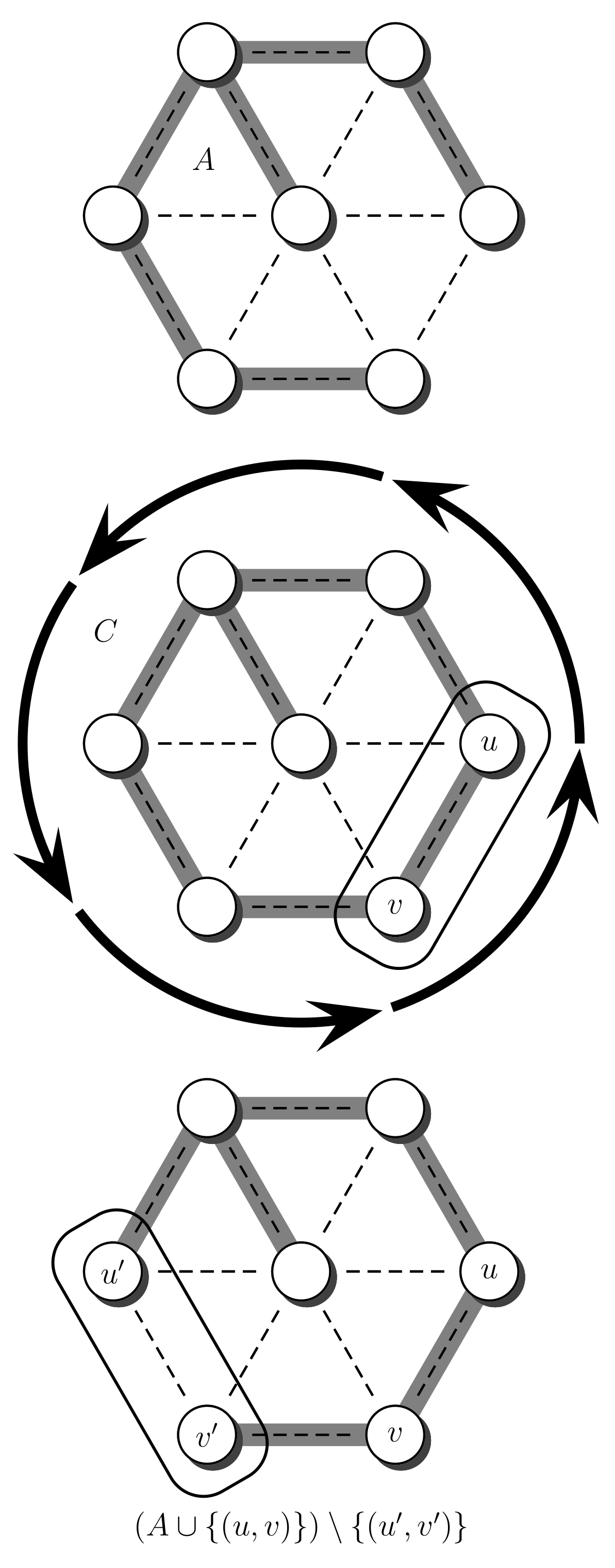
Figure 4.
Schematic representation of the relations between , , and I.

Figure 5.
Case 2.

Figure 6.
Case 3.
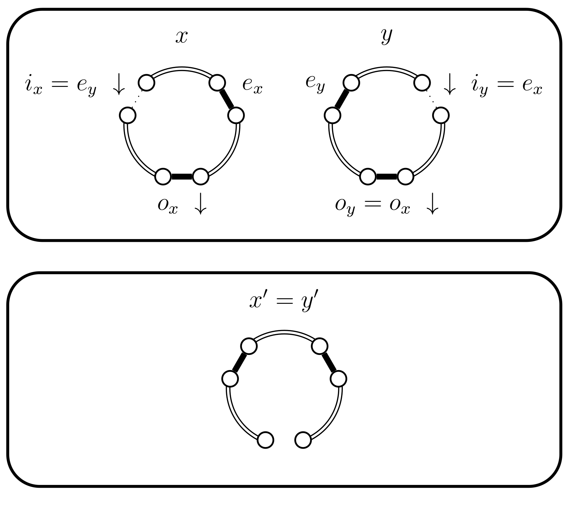
Figure 7.
Case 4.a.i, case 4.b.i, and case 4.c.i.

Figure 8.
Case 4.a.ii, case 4.b.ii, and case 4.c.ii, when .

Figure 9.
Case 4.a.ii, case 4.b.ii, and case 4.c.ii, when .

Figure 10.
Case 4.a.iii, case 4.b.iv, and case 4.c.iv, when is true.
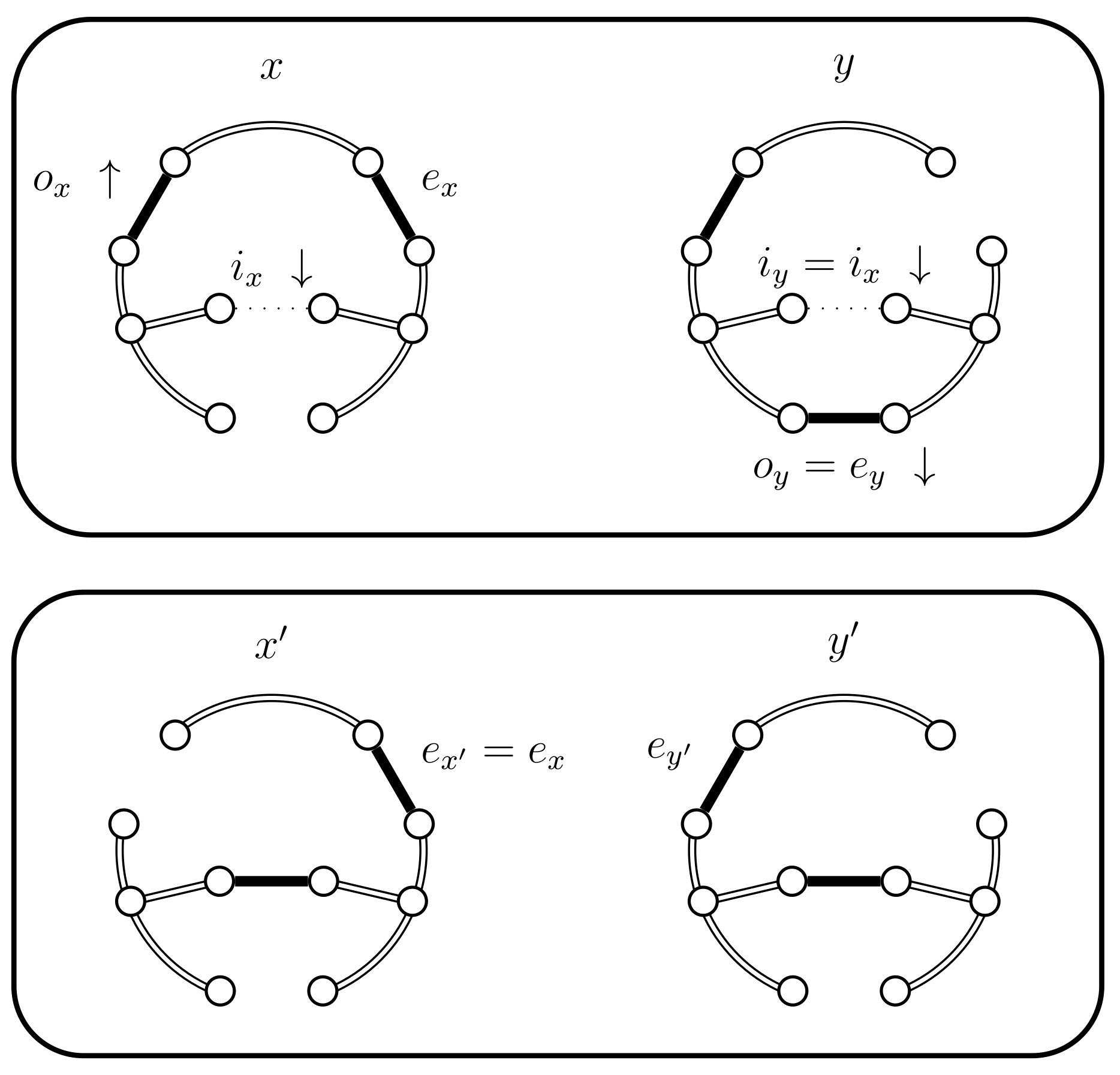
Figure 11.
Case 4.a.iv, case 4.b.iv, and case 4.c.iv.

Figure 12.
Case 4.b.i when B fails and .

Figure 13.
Case 4.b.ii.
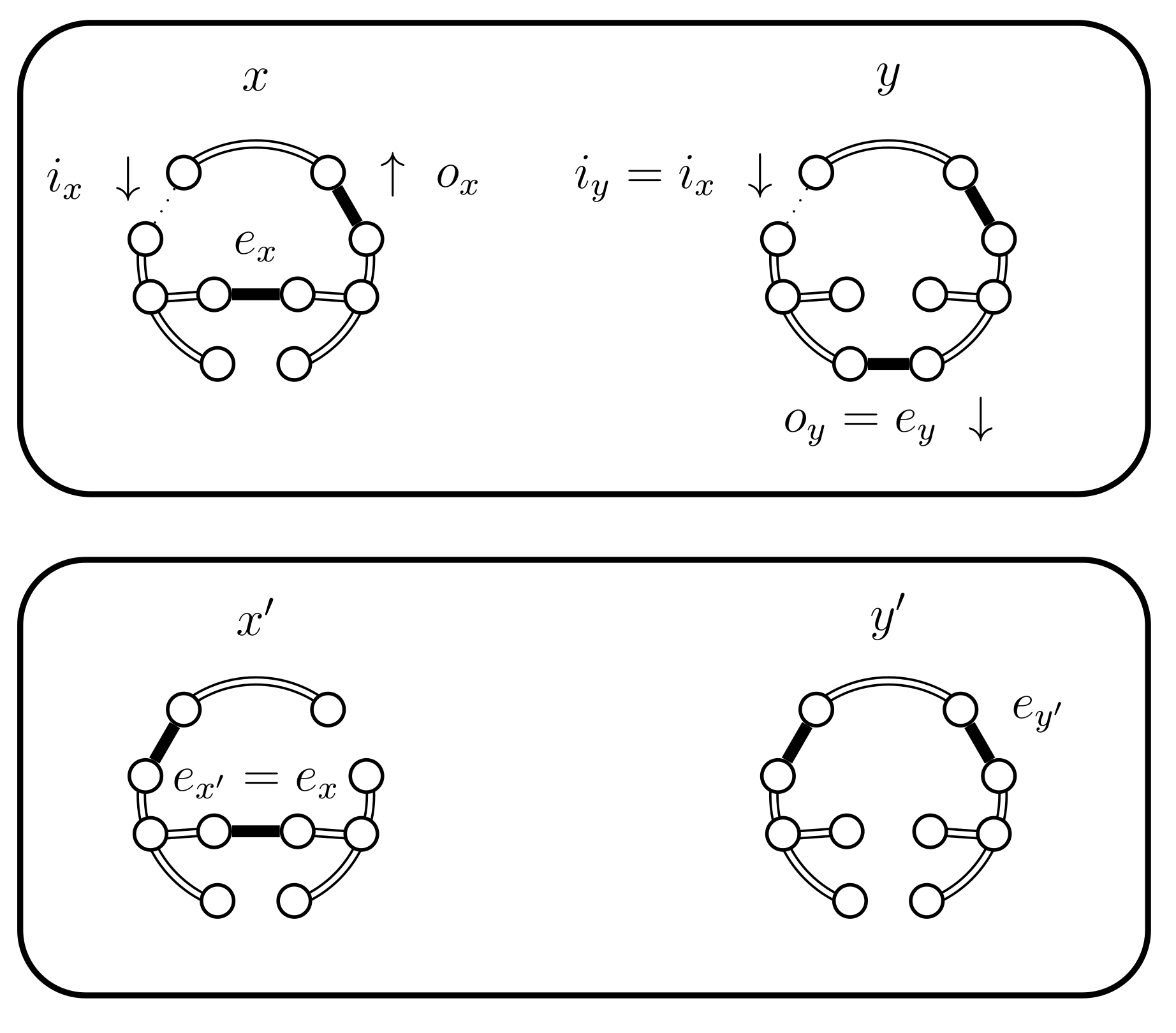
Figure 14.
Case 4.b.iii.
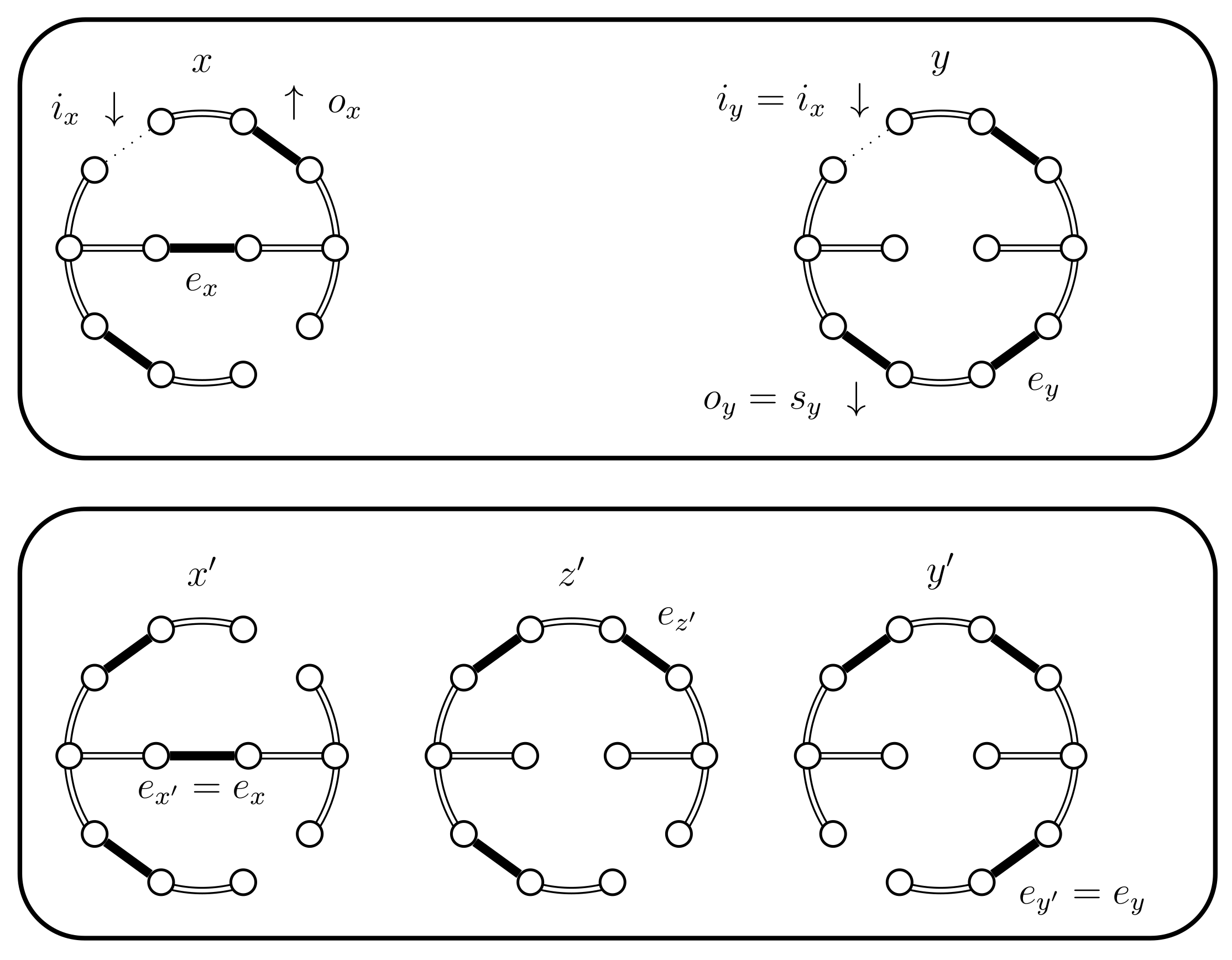
Figure 15.
Case 4.c.iii, when is true.

Figure 16.
A cycle graph.

Figure 17.
Cycles connected by bridges or articulation points.

Figure 18.
Estimation of variation distance as a function of the number of iterations for sparse graphs (see Section 4.3.1 for details).
Figure 18.
Estimation of variation distance as a function of the number of iterations for sparse graphs (see Section 4.3.1 for details).
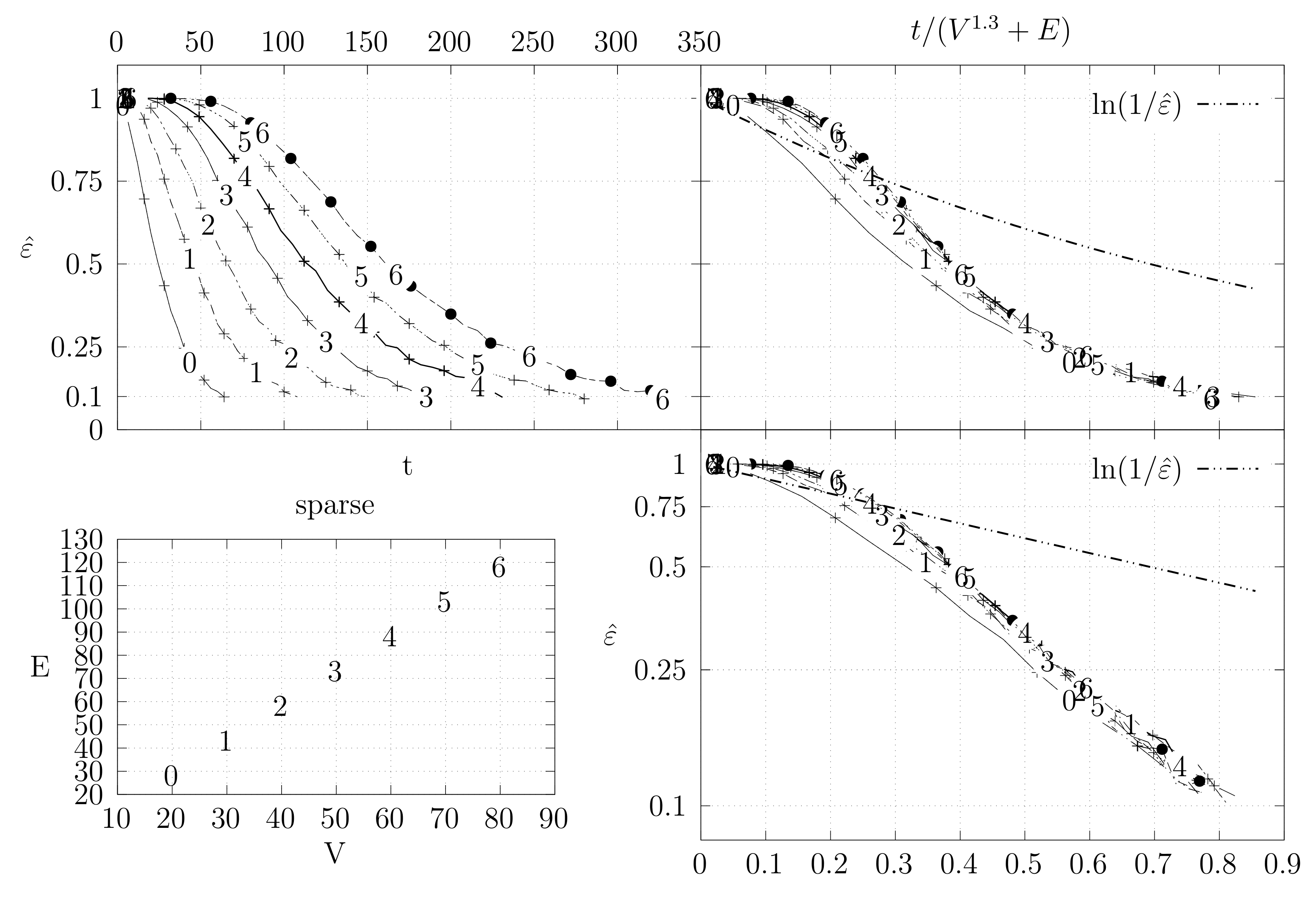
Figure 19.
Estimation of variation distance as a function of the number of iterations for cycle graphs (see Section 4.3.1 for details).
Figure 19.
Estimation of variation distance as a function of the number of iterations for cycle graphs (see Section 4.3.1 for details).
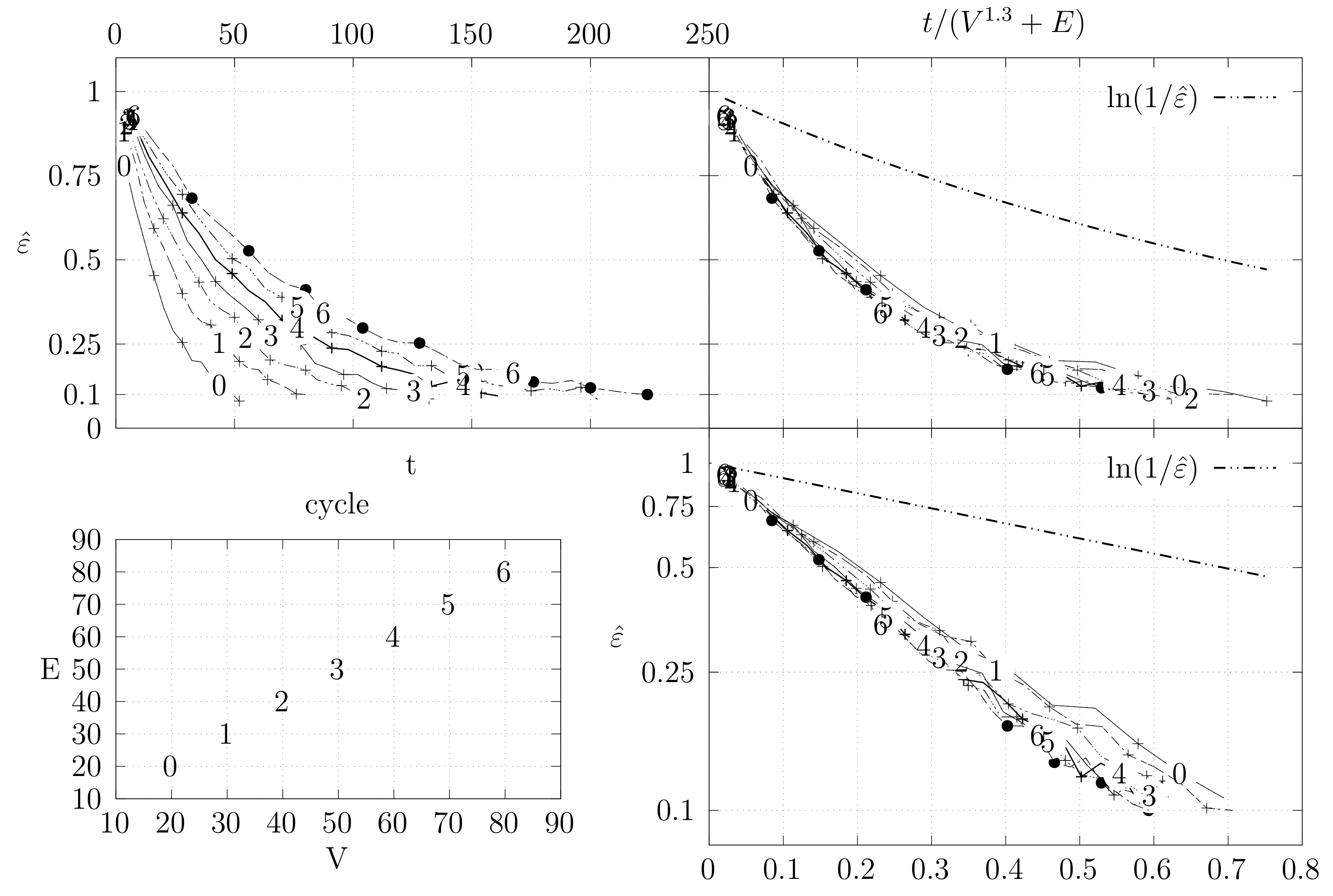
Figure 20.
Estimation of variation distance as a function of the number of iterations for dense graphs (see Section 4.3.1 for details).
Figure 20.
Estimation of variation distance as a function of the number of iterations for dense graphs (see Section 4.3.1 for details).
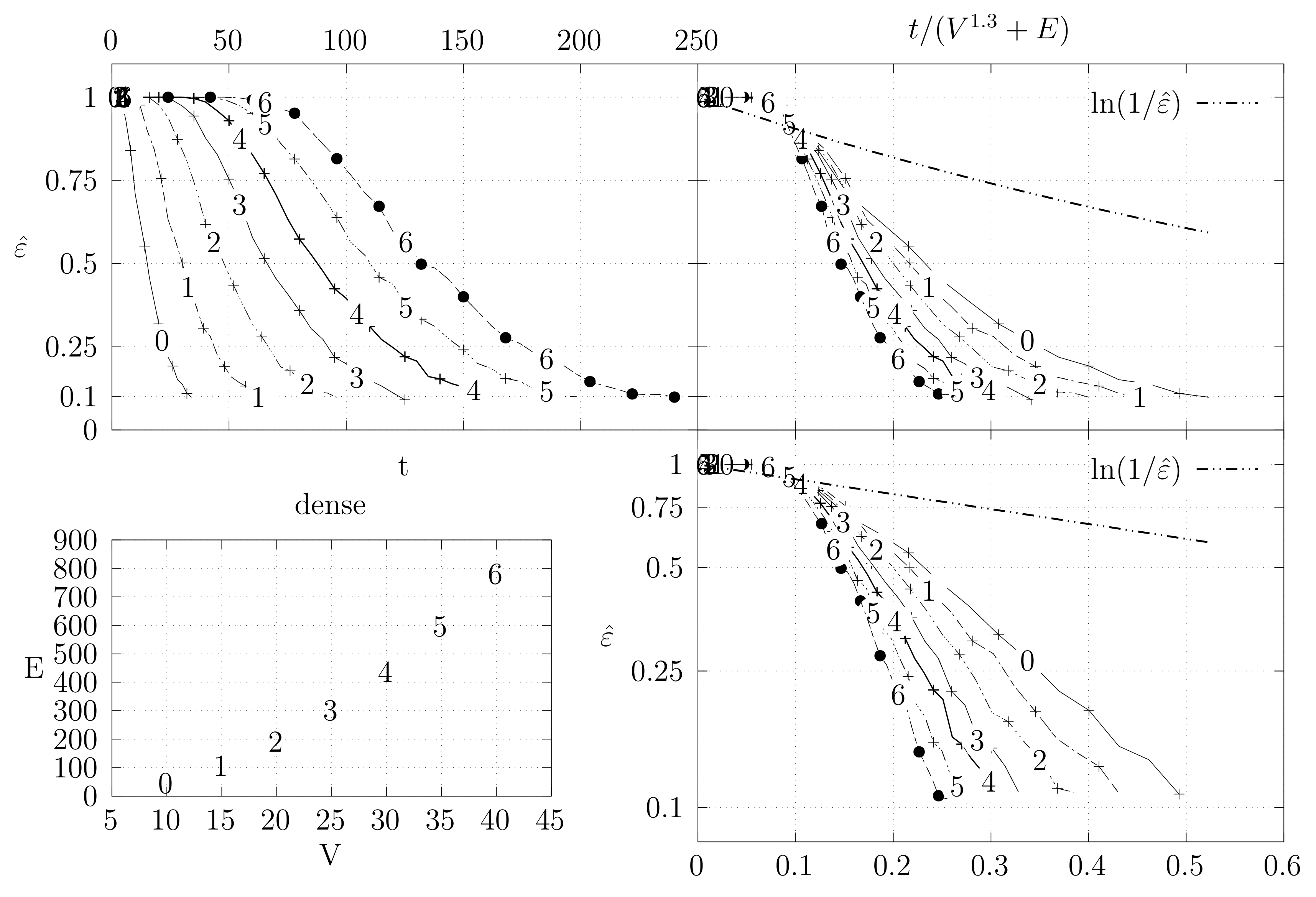
Figure 21.
Estimation of variation distance as a function of the number of iterations for biK graphs (see Section 4.3.1 for details).
Figure 21.
Estimation of variation distance as a function of the number of iterations for biK graphs (see Section 4.3.1 for details).

Figure 22.
Estimation of variation distance as a function of the number of iterations for dmP graphs (see Section 4.3.1 for details).
Figure 22.
Estimation of variation distance as a function of the number of iterations for dmP graphs (see Section 4.3.1 for details).

Figure 23.
Estimation of variation distance as a function of the number of iterations for dmP graphs (see Section 4.3.1 for details).
Figure 23.
Estimation of variation distance as a function of the number of iterations for dmP graphs (see Section 4.3.1 for details).

Figure 24.
Estimation of variation distance as a function of the number of iterations for dmP graphs (see Section 4.3.1 for details).
Figure 24.
Estimation of variation distance as a function of the number of iterations for dmP graphs (see Section 4.3.1 for details).
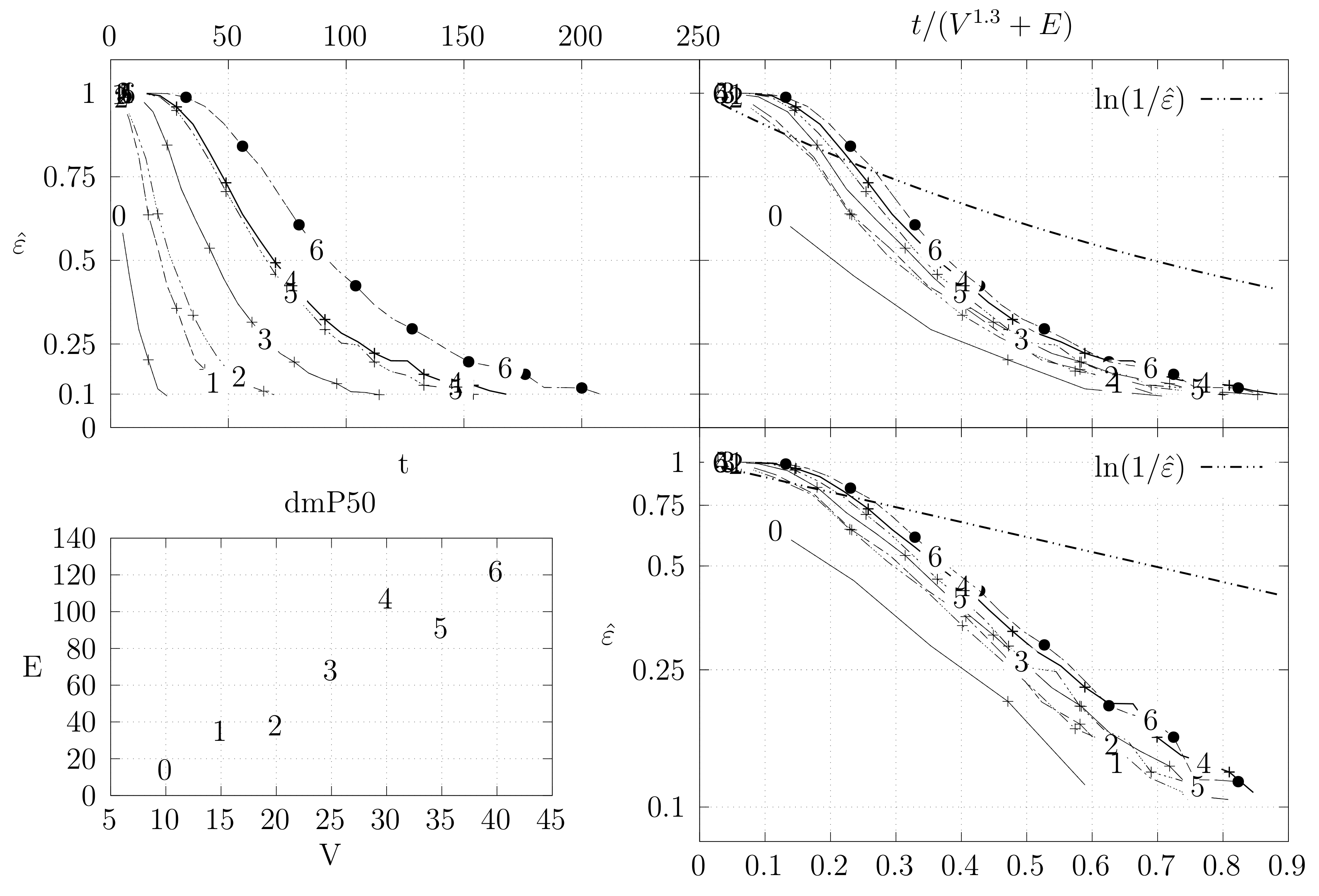
Figure 25.
A ladder graph.
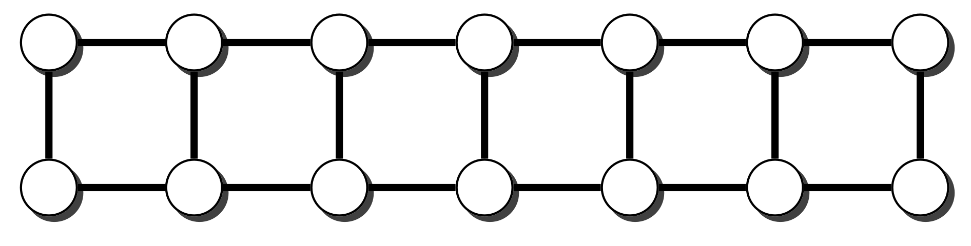
Figure 26.
Running times for dense (fully connected) graphs averaged over five runs, including the running time for computing the optimistic coupling estimate and the running time for generating a spanning tree based on that estimate, as well as the edge-swapping algorithm, the running time for generating a spanning tree through a random walk, and the running time for Wilson’s algorithm.

Figure 27.
Running times for biK graphs averaged over five runs, including the running time for computing the optimistic coupling estimate, the running time for generating a spanning tree based on that estimate, the edge-swapping algorithm, the running time for generating a spanning tree through a random walk, and the running time for Wilson’s algorithm.
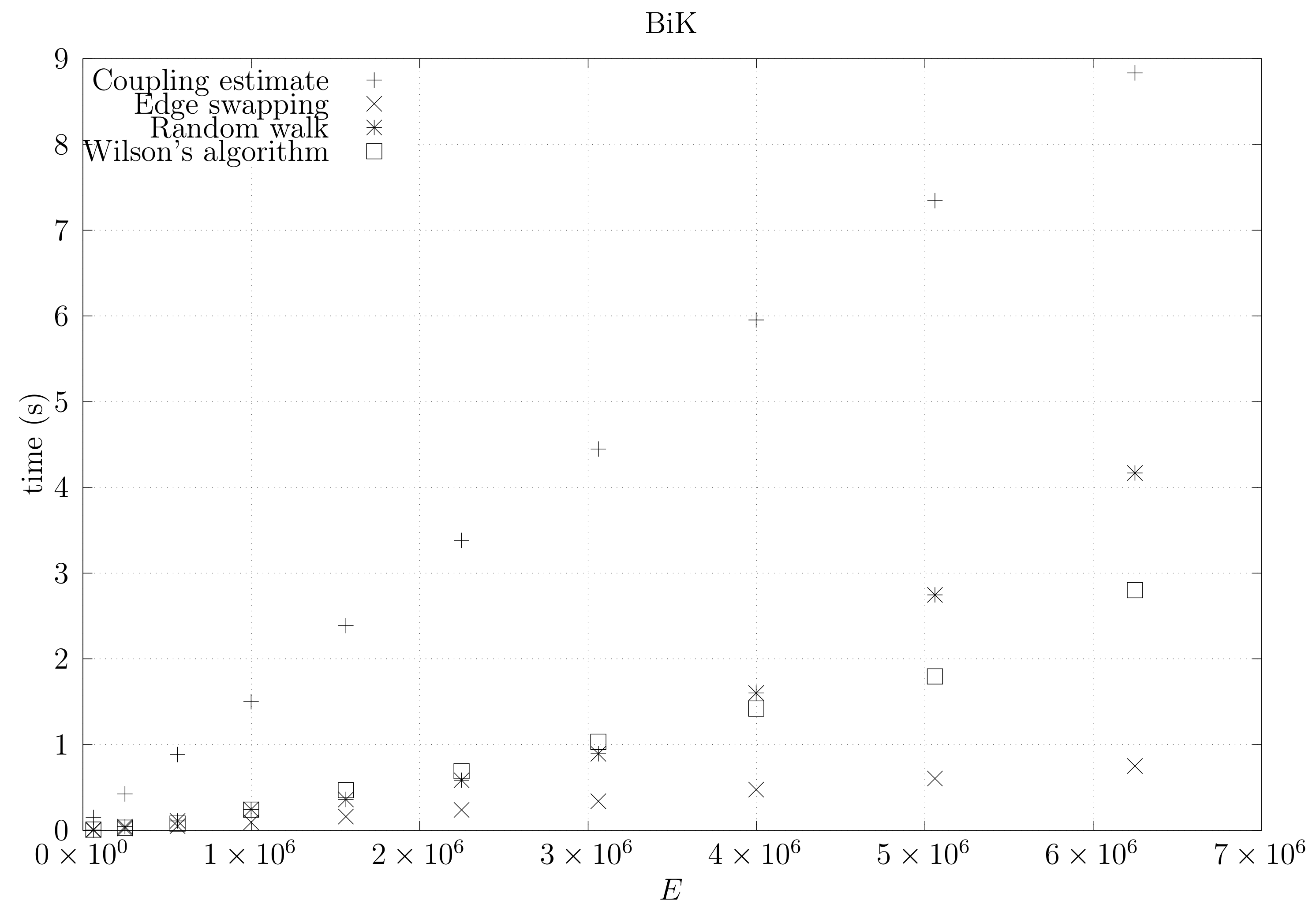
Figure 28.
Running times for cycle graphs averaged over five runs, including the running time for computing the optimistic coupling estimate, the running time for generating a spanning tree based on that estimate, the edge-swapping algorithm, the running time for generating a spanning tree through a random walk, and the running time for Wilson’s algorithm.
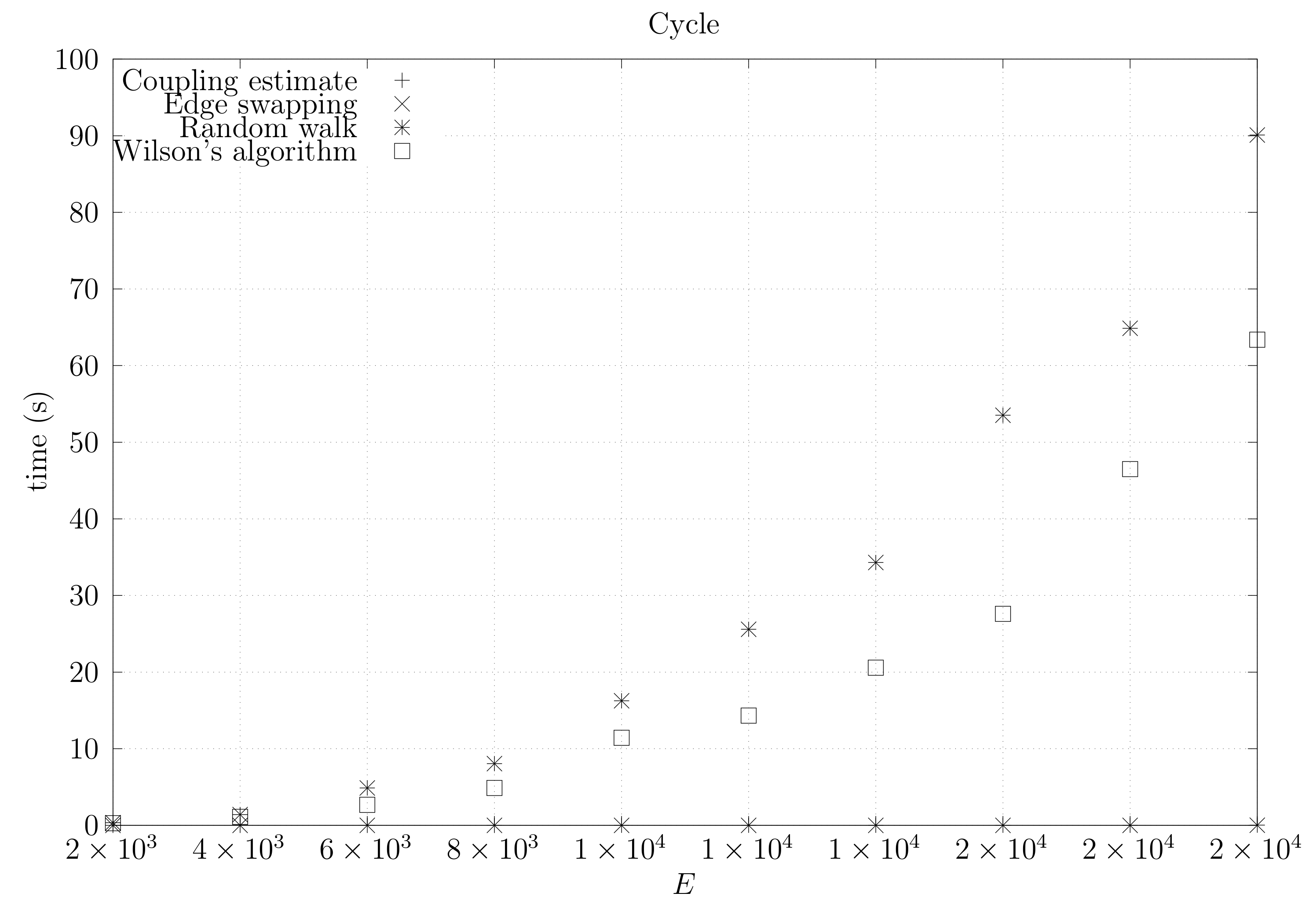
Figure 29.
Running times for sparse (ladder) graphs averaged over five runs, including the running time for computing the optimistic coupling estimate, the running time for generating a spanning tree based on that estimate, the edge-swapping algorithm, the running time for generating a spanning tree through a random walk, and the running time for Wilson’s algorithm.

Figure 30.
Running times for square torus graphs averaged over five runs, including the running time for computing the optimistic coupling estimate, the running time for generating a spanning tree based on that estimate, the edge-swapping algorithm, the running time for generating a spanning tree through a random walk, and the running time for Wilson’s algorithm.

Figure 31.
Running times for rectangular torus graphs averaged over five runs, including the running time for computing the optimistic coupling estimate, the running time for generating a spanning tree based on that estimate, the edge-swapping algorithm, the running time for generating a spanning tree through a random walk, and the running time for Wilson’s algorithm.

Figure 32.
Running times for dmP graphs averaged over five runs, including the running time for computing the optimistic coupling estimate, the running time for generating a spanning tree based on that estimate, the edge-swapping algorithm, the running time for generating a spanning tree through a random walk, and the running time for Wilson’s algorithm.

Table 1.
Variation distance (VD) for different graph topologies. Median and maximum VD computed over five runs for each network. Since dmP graphs are random, results for dmP were further computed over five different graphs for each size .
Table 1.
Variation distance (VD) for different graph topologies. Median and maximum VD computed over five runs for each network. Since dmP graphs are random, results for dmP were further computed over five different graphs for each size .
| Graph | Median VD | Max VD | |
|---|---|---|---|
| dense | 0.060 | 0.194 | |
| biK | 0.065 | 0.190 | |
| cycle | 0.001 | 0.004 | |
| sparse | 0.053 | 0.110 | |
| torus | 0.094 | 0.383 | |
| dmP | 0.069 | 0.270 |
© 2018 by the authors. Licensee MDPI, Basel, Switzerland. This article is an open access article distributed under the terms and conditions of the Creative Commons Attribution (CC BY) license (http://creativecommons.org/licenses/by/4.0/).
Share and Cite
MDPI and ACS Style
Russo, L.M.S.; Teixeira, A.S.; Francisco, A.P. Linking and Cutting Spanning Trees. Algorithms 2018, 11, 53. https://doi.org/10.3390/a11040053
AMA Style
Russo LMS, Teixeira AS, Francisco AP. Linking and Cutting Spanning Trees. Algorithms. 2018; 11(4):53. https://doi.org/10.3390/a11040053
Chicago/Turabian StyleRusso, Luís M. S., Andreia Sofia Teixeira, and Alexandre P. Francisco. 2018. "Linking and Cutting Spanning Trees" Algorithms 11, no. 4: 53. https://doi.org/10.3390/a11040053
Note that from the first issue of 2016, this journal uses article numbers instead of page numbers. See further details here.