A Novel Method for Control Performance Assessment with Fractional Order Signal Processing and Its Application to Semiconductor Manufacturing


Abstract
:1. Introduction
- Use MFDFA to analyze semiconductor data, derive the multifractal spectrum and select the characteristic parameters sensitive to changes of the control system.
- Extract the characteristic parameters from the multifractal spectrum of reference data to form reference feature sets;
- Modify the standard single Hurst exponent estimation by the multiple Hurst exponent fitting method with crossover points;
- Select multifractal properties and modified Hurst exponents to distinguish different types of control actions (tunings).
2. Preliminaries
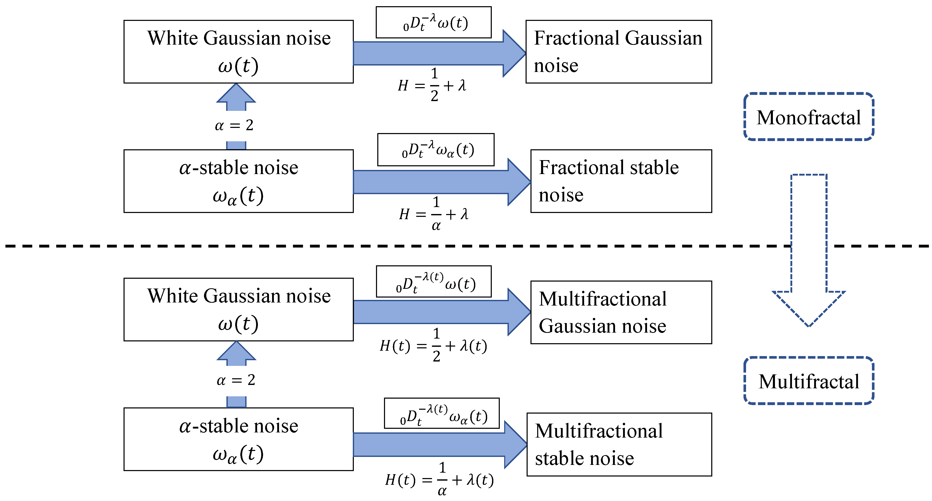
2.1. Fractal and Fractional Gaussian Noise
2.2. Hurst Parameter
2.3. Stable Distribution
3. MFDFA Algorithm
3.1. Basic MFDFA Algorithm
- Define the “profile” E and transform original data into mean-reduced cumulative sums,where is the mean of series, such that the aggregated time series are with zero mean.
- Divide time series into non-overlapping segments of equal length s, starting from the beginning. Since the length N of the series is often not a multiple of the considered time scale s, in order to not miss any piece of data, another set of segments starting from the end of data is made from the end coming to the beginning. As a result, segments are obtained covering the whole dataset.
- Calculate the local trend for each of the segments by a least-square fit of the series.
- Calculate the mean square error for the estimate of each segment k of length s.for each segment andfor each segment .
- Average over all segments to obtain the qth order variance (or fluctuation) function for each size s:For use
- Repeat steps (2)–(5) for different s evaluating new sets of variances .
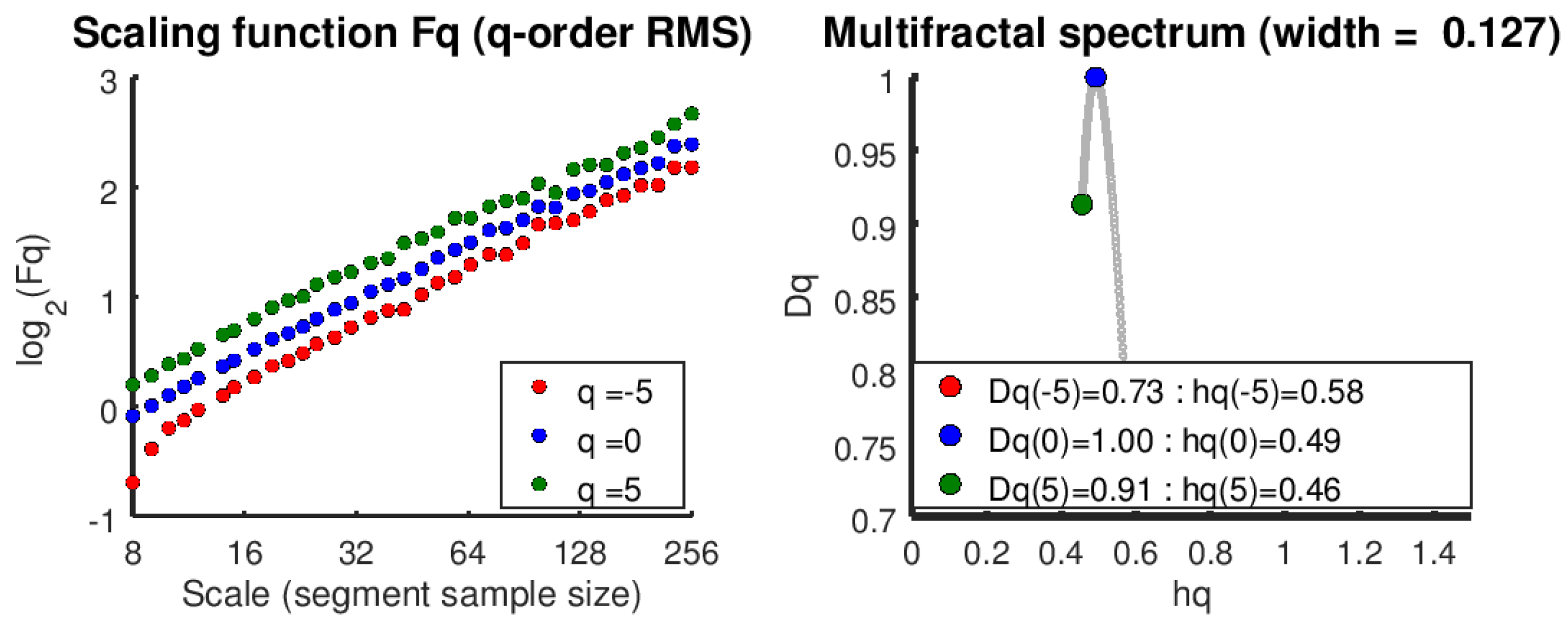
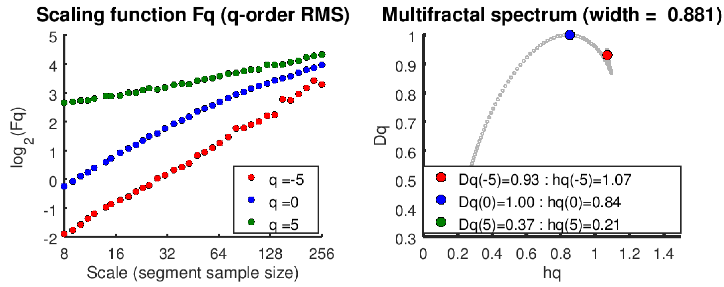
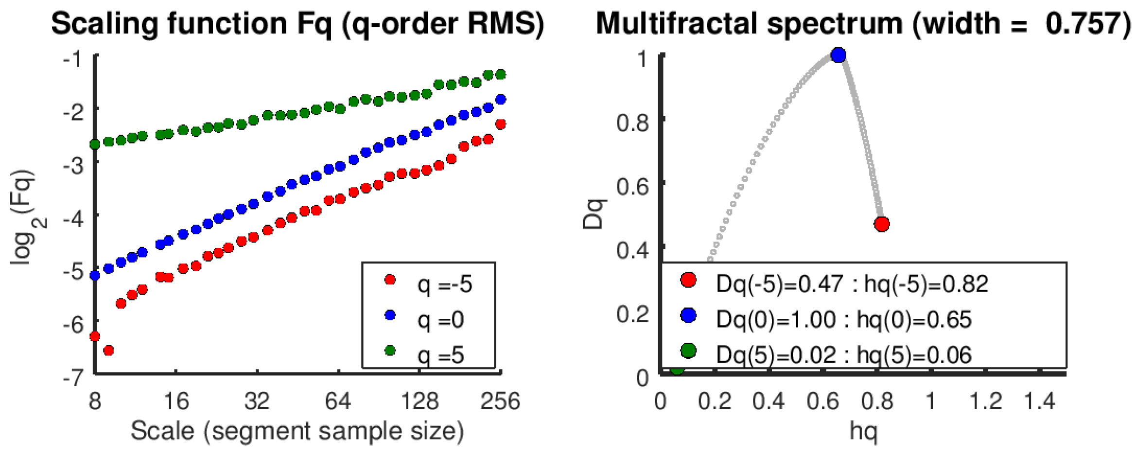
- Plot for each q in log-log scale and estimate the linear fit with least squares. If slope varies with q, multifractality is suspected. Single slope shows monofractal scaling.
- Calculate multifractal exponent as
- Use Legendre transform to evaluate Hölder exponent and multifractal spectrum :
3.2. Defining the Source of the Multifractality
3.3. Plot Fitting Hurst Exponents with Crossovers
4. Case Studies
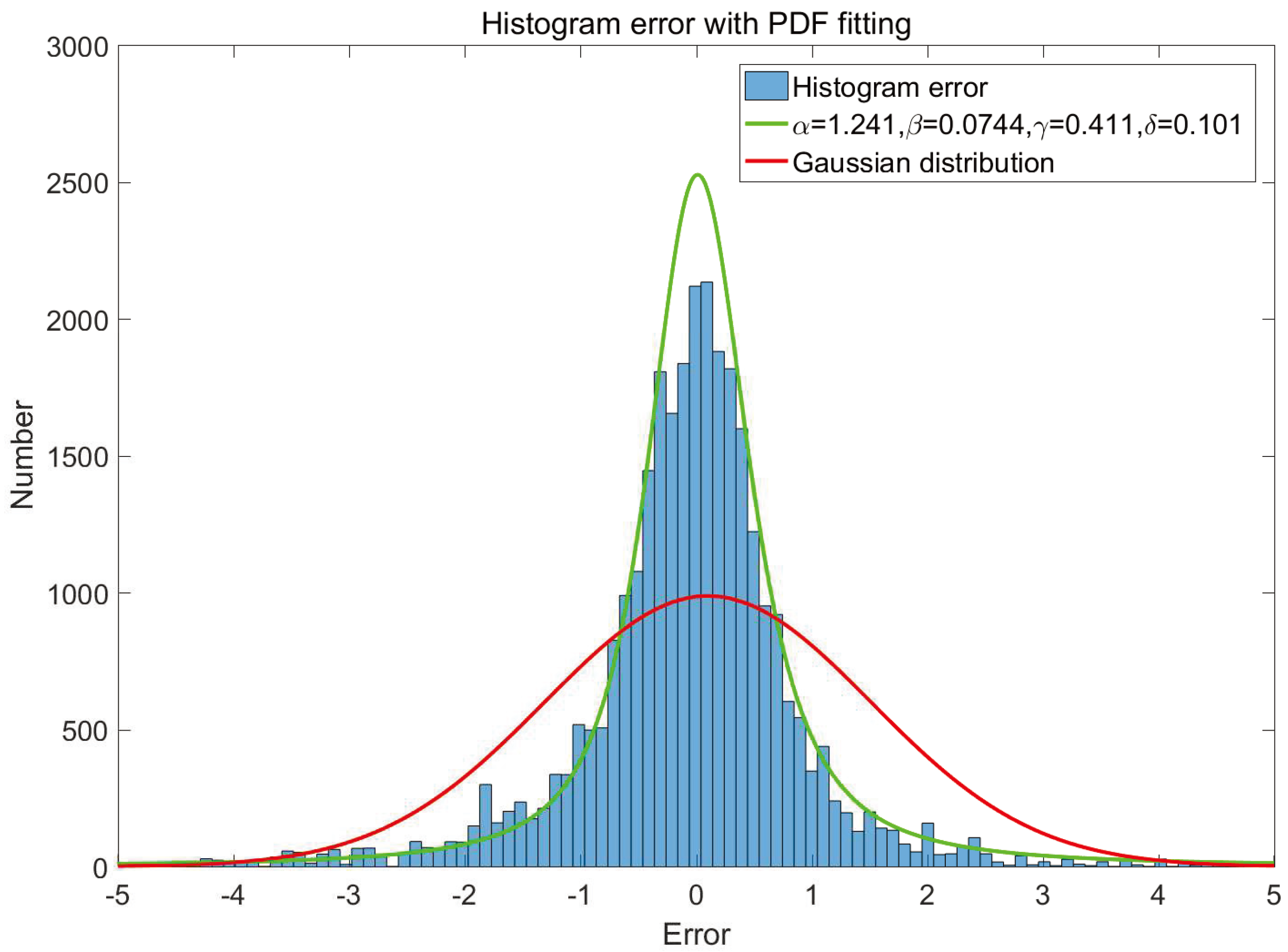
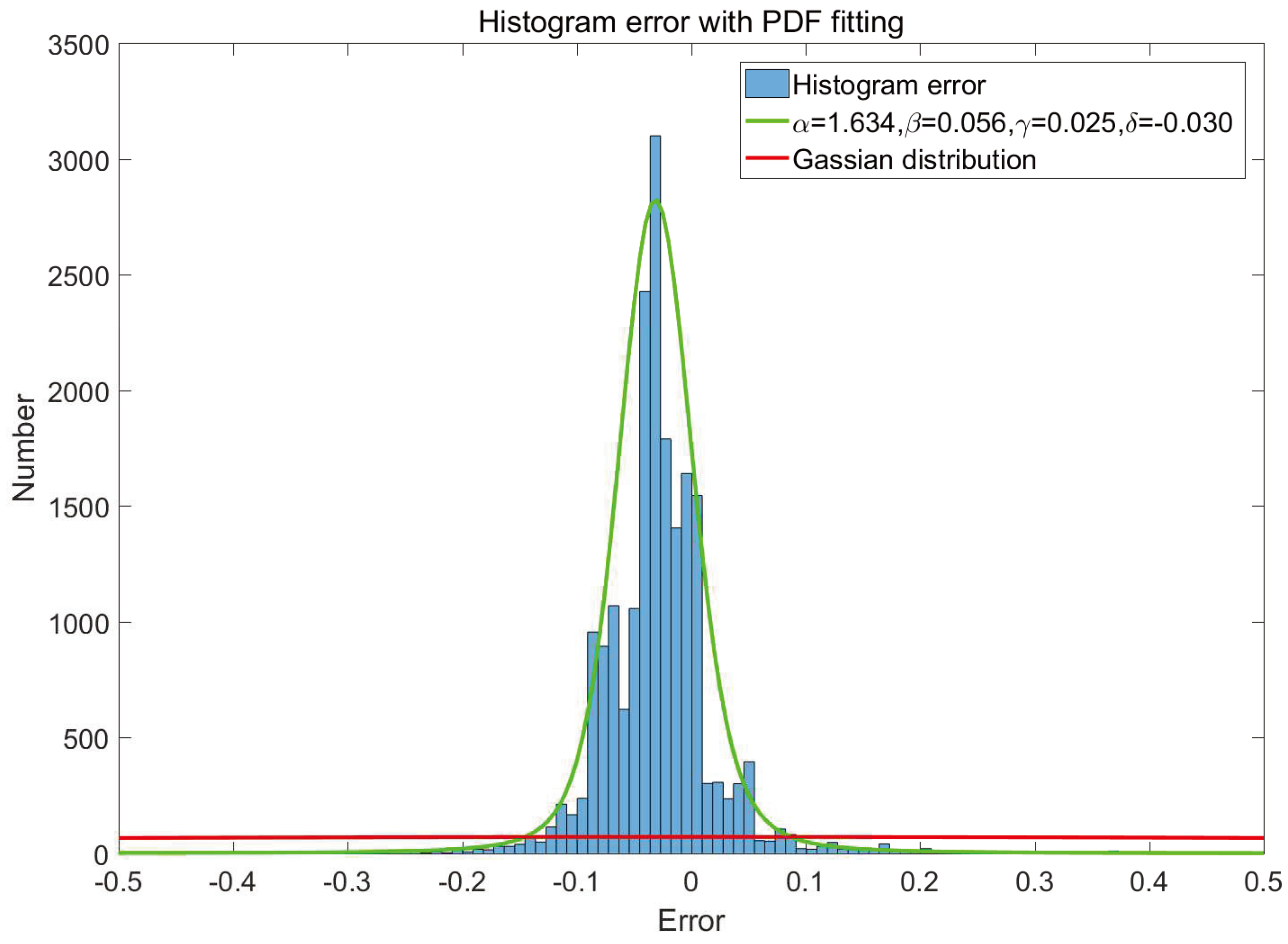
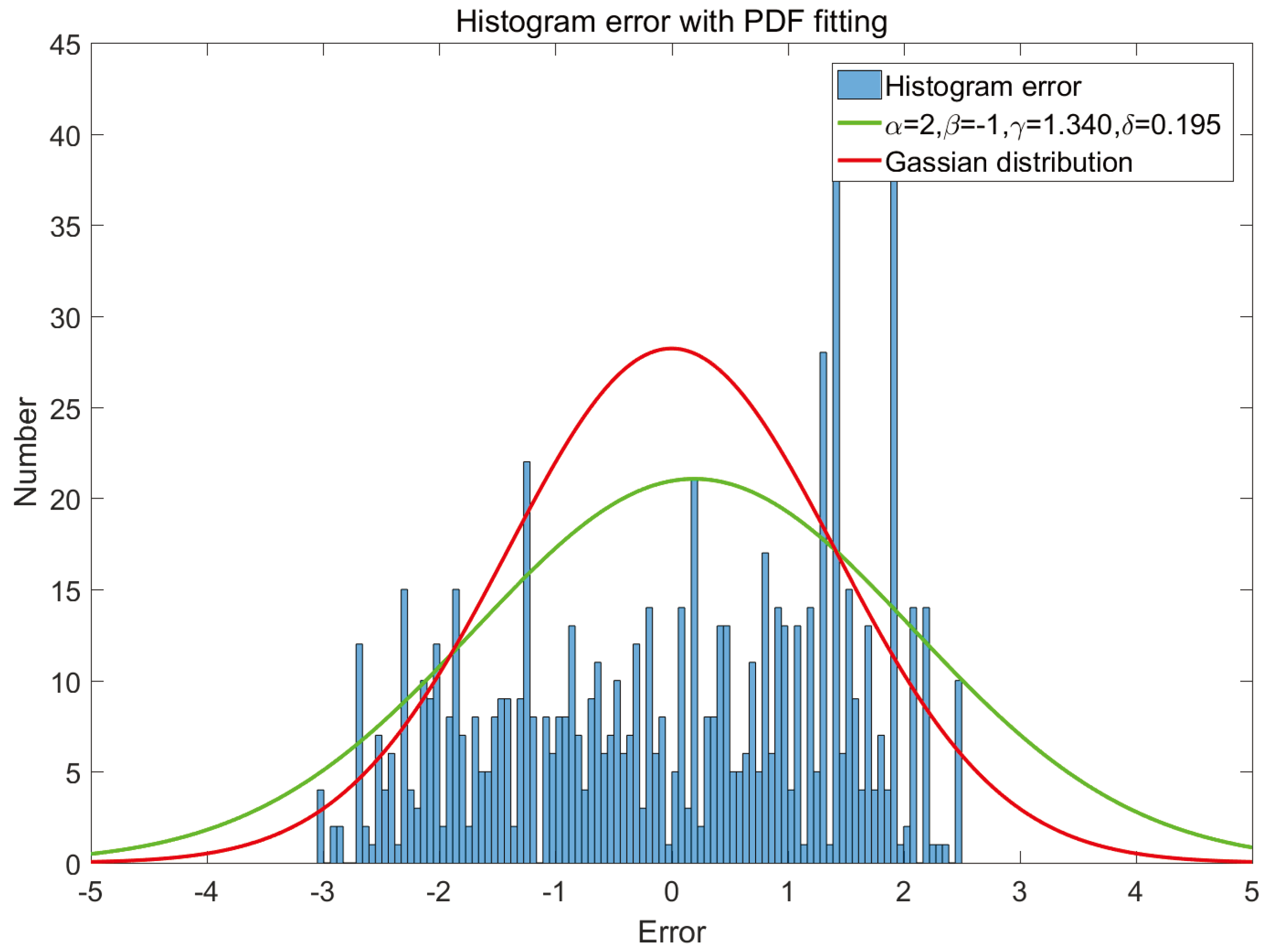
4.1. Non-Gaussian Statistical Analysis
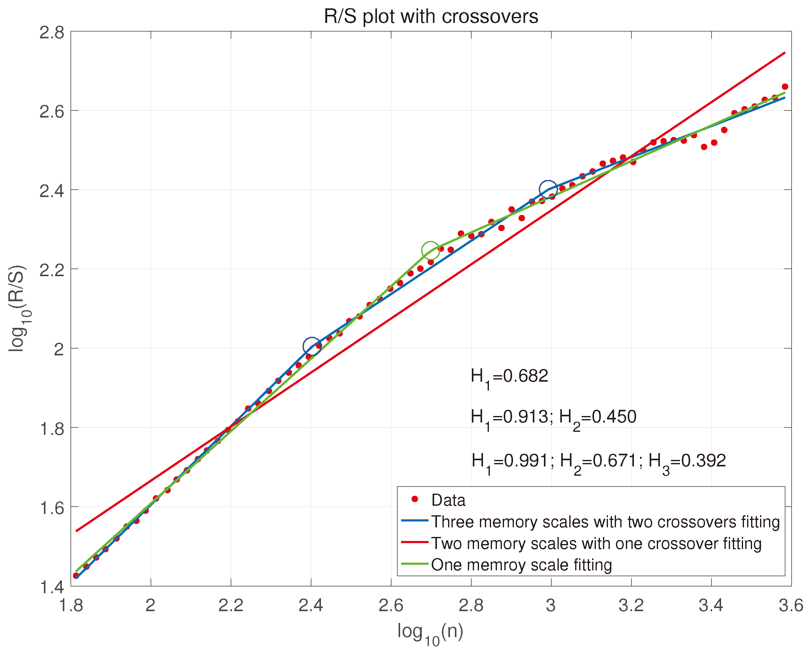
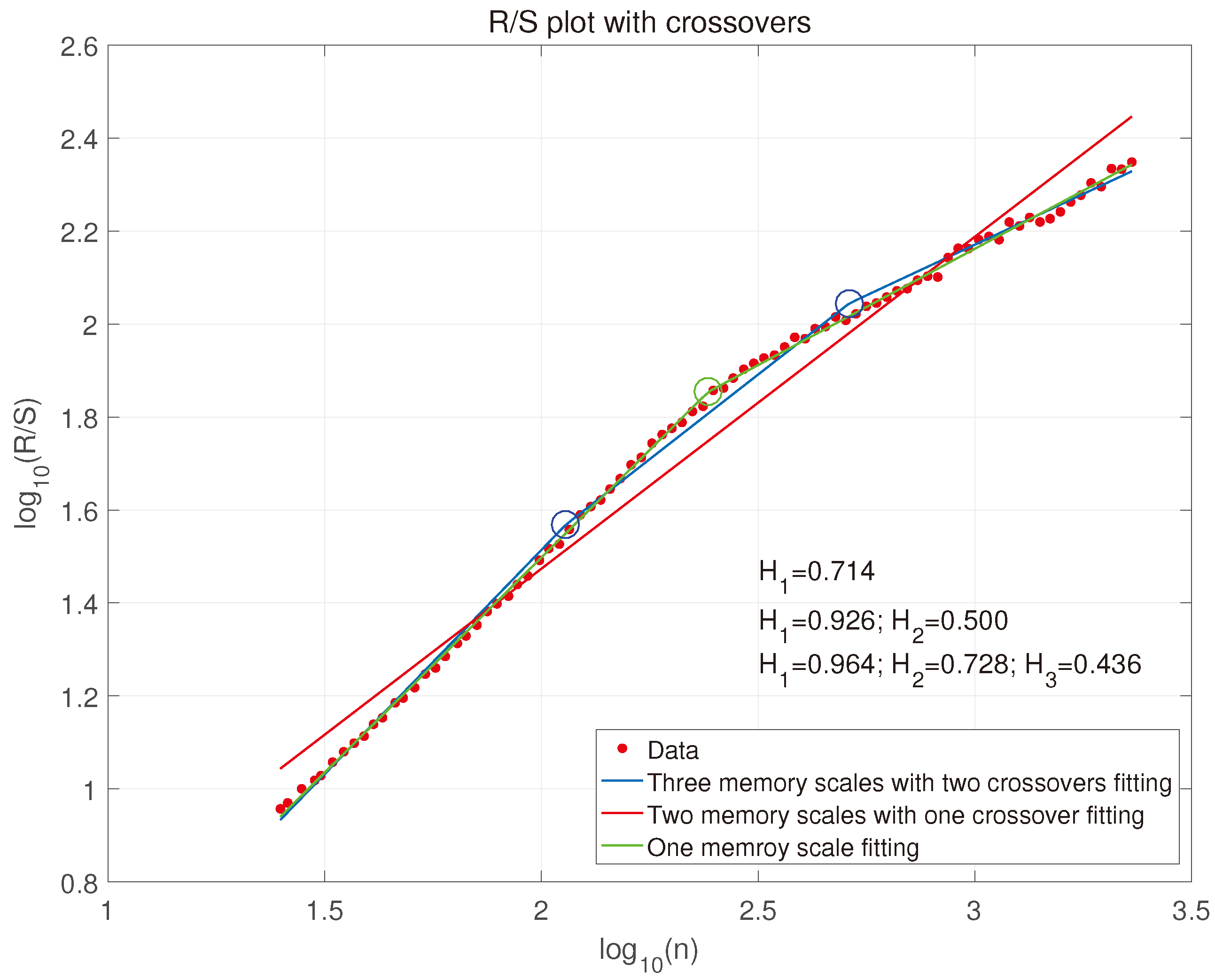
4.2. Hurst Exponents Fitting with Crossovers
4.3. Multifractal Analysis
5. Results and Discussion
6. Conclusions
Author Contributions
Funding
Conflicts of Interest
References
- Jelali, M. Control Performance Management in Industrial Automation: Assessment, Diagnosis and Improvement of Control Loop Performance; Springer Science & Business Media: London, UK, 2012. [Google Scholar]
- Sheng, H.; Chen, Y.; Qiu, T. Fractional Processes and Fractional-Order Signal Processing: Techniques and Applications; Springer Science & Business Media: London, UK, 2011. [Google Scholar]
- Chen, Y.; Sun, R.; Zhou, A. An overview of fractional order signal processing (FOSP) techniques. In Proceedings of the International Design Engineering Technical Conferences and Computers and Information in Engineering Conference, Las Vegas, NV, USA, 4–7 September 2007; pp. 1205–1222. [Google Scholar]
- West, B.J. Fractional Calculus View of Complexity: Tomorrow’s Science; CRC Press: Boca Raton, FL, USA, 2016. [Google Scholar]
- Jelali, M. An overview of control performance assessment technology and industrial applications. Control Eng. Pract. 2006, 14, 441–466. [Google Scholar] [CrossRef]
- Domański, P.D. On-line control loop assessment with non-Gaussian statistical and fractal measures. In Proceedings of the American Control Conference (ACC), Seattle, WA, USA, 24–26 May 2017; pp. 555–560. [Google Scholar]
- Domański, P.D. Multifractal Properties of Process Control Variables. Int. J. Bifurc. Chaos 2017, 27, 1750094. [Google Scholar] [CrossRef]
- Domański, P.D.; Ławryńczuk, M. Assessment of predictive control performance using fractal measures. Nonlinear Dyn. 2017, 89, 773–790. [Google Scholar] [CrossRef] [Green Version]
- Mandelbrot, B.B. The Fractal Geometry of Nature; Freeman: New York, NY, USA, 1983. [Google Scholar]
- Feder, J. Fractals; Springer Science & Business Media: London, UK, 2013. [Google Scholar]
- Schmitt, D.T.; Ivanov, P.C. Fractal scale-invariant and nonlinear properties of cardiac dynamics remain stable with advanced age: A new mechanistic picture of cardiac control in healthy elderly. Am. J. Physiol. Regul. Integr. Comp. Physiol. 2007, 293, R1923–R1937. [Google Scholar] [CrossRef] [PubMed]
- Kilbas, A.A.; Saigo, M.; Saxena, R. Generalized Mittag-Leffler function and generalized fractional calculus operators. Integral Transf. Spec. Funct. 2004, 15, 31–49. [Google Scholar] [CrossRef]
- Mainardi, F. Fractional Calculus and Waves in Linear Viscoelasticity: An Introduction to Mathematical Models; Imperial College Press: London, UK, 2010. [Google Scholar]
- Podlubny, I. Fractional Differential Equations: An Introduction to Fractional Derivatives, Fractional Differential Equations, to Methods of Their Solution and Some of Their Applications; Academic Press: San Diego, CA, USA, 1998; Volume 198. [Google Scholar]
- Mandelbrot, B.B.; van Ness, J.W. Fractional Brownian motions, fractional noises and applications. SIAM Rev. 1968, 10, 422–437. [Google Scholar] [CrossRef]
- Hurst, H.E. Long-term storage capacity of reservoirs. Trans. Am. Soc. Civ. Eng. 1951, 116, 770–808. [Google Scholar]
- Samorodnitsky, G.; Taqqu, M.S. Stable Non-Gaussian Random Processes: Stochastic Models with Infinite Variance; CRC Press: Boca Raton, FL, USA, 1994; Volume 1. [Google Scholar]
- Ye, X.; Xia, X.; Zhang, J.; Chen, Y. Effects of trends and seasonalities on robustness of the Hurst parameter estimators. IET Signal Process. 2012, 6, 849–856. [Google Scholar] [CrossRef] [Green Version]
- Inoue, A. Asymptotic behavior for partial autocorrelation functions of fractional ARIMA processes. Ann. Appl. Probabil. 2002, 12, 1471–1491. [Google Scholar] [CrossRef]
- Woodward, W.A.; Gray, H.L.; Elliott, A.C. Applied Time Series Analysis with R, 2nd ed.; CRC Press: Boca Raton, FL, USA, 2016. [Google Scholar]
- Liu, K.; Chen, Y.; Zhang, X. An Evaluation of ARFIMA (Autoregressive Fractional Integral Moving Average) Programs. Axioms 2017, 6, 16. [Google Scholar] [CrossRef]
- Gorenflo, R.; Mainardi, F. Fractional calculus and stable probability distributions. Arch. Mech. 1998, 50, 377–388. [Google Scholar]
- Nikias, C.L.; Shao, M. Signal Processing With Alpha-Stable Distributions and Applications; Wiley-Interscience: New York, NY, USA, 1995. [Google Scholar]
- Koutrouvelis, I.A. Regression-type estimation of the parameters of stable laws. J. Am. Stat. Assoc. 1980, 75, 918–928. [Google Scholar] [CrossRef]
- McCulloch, J.H. Simple consistent estimators of stable distribution parameters. Commun. Stat. Simul. Comput. 1986, 15, 1109–1136. [Google Scholar] [CrossRef]
- Movahed, M.S.; Jafari, G.; Ghasemi, F.; Rahvar, S.; Tabar, M.R.R. Multifractal detrended fluctuation analysis of sunspot time series. J. Stat. Mech. Theory Exp. 2006, 2006, P02003. [Google Scholar] [CrossRef]
- Srinivasan, B.; Spinner, T.; Rengaswamy, R. Control loop performance assessment using detrended fluctuation analysis (DFA). Automatica 2012, 48, 1359–1363. [Google Scholar] [CrossRef]
- Zhang, Q.; Xu, C.Y.; Chen, Y.D.; Yu, Z. Multifractal detrended fluctuation analysis of streamflow series of the Yangtze River basin, China. Hydrol. Process. 2008, 22, 4997–5003. [Google Scholar] [CrossRef]
- Telesca, L.; Lovallo, M. Analysis of the time dynamics in wind records by means of multifractal detrended fluctuation analysis and the Fisher–Shannon information plane. J. Stat. Mech. Theory Exp. 2011, 7, P07001. [Google Scholar] [CrossRef]
- Wang, Y.; Wei, Y.; Wu, C. Analysis of the efficiency and multifractality of gold markets based on multifractal detrended fluctuation analysis. Phys. A Stat. Mech. Appl. 2011, 390, 817–827. [Google Scholar] [CrossRef]
- Shang, P.; Lu, Y.; Kamae, S. Detecting long-range correlations of traffic time series with multifractal detrended fluctuation analysis. Chaos Solitons Fractals 2008, 36, 82–90. [Google Scholar] [CrossRef]
- Lin, J.; Chen, Q. Fault diagnosis of rolling bearings based on multifractal detrended fluctuation analysis and Mahalanobis distance criterion. Mech. Syst. Signal Process. 2013, 38, 515–533. [Google Scholar] [CrossRef]
- Peng, C.K.; Havlin, S.; Stanley, H.E.; Goldberger, A.L. Quantification of scaling exponents and crossover phenomena in nonstationary heartbeat time series. Chaos 1995, 5, 82–87. [Google Scholar] [CrossRef] [PubMed]
- Kantelhardt, J.W.; Zschiegner, S.A.; Koscielny-Bunde, E.; Havlin, S.; Bunde, A.; Stanley, H.E. Multifractal detrended fluctuation analysis of nonstationary time series. Phys. A Stat. Mech. Appl. 2002, 316, 87–114. [Google Scholar] [CrossRef] [Green Version]
- Ihlen, E.A. Introduction to multifractal detrended fluctuation analysis in Matlab. Front. Physiol. 2012, 3, 141. [Google Scholar] [CrossRef] [PubMed]


| Variables | |||||||
|---|---|---|---|---|---|---|---|
| Var1 | 1.241 | 0.074 | 0.411 | 0.101 | 1.07 | 0.21 | 0.881 |
| Var2 | 1.634 | 0.056 | 0.025 | −0.030 | 0.82 | 0.06 | 0.757 |
| Var3 | 2.000 | −1.000 | 0.456 | −0.235 | 0.58 | 0.46 | 0.127 |
| Var1’ | 1.171 | −0.156 | 0.456 | −0.235 | 1.04 | 0.25 | 0.798 |
| Var2’ | 1.695 | 0.287 | 0.123 | −0.246 | 0.71 | 0.41 | 0.307 |
| Var3’ | 2.000 | 1.000 | 1.567 | −0.208 | 0.57 | 0.53 | 0.069 |
| Variables | |||
|---|---|---|---|
| Var1 | 0.682 | 0.913, 0.450 | 0.991, 0.671, 0.392 |
| Var2 | 0.714 | 0.926, 0.500 | 0.964, 0.728, 0.436 |
| Var3 | 1.010 | 1.044, 0.974 | 1.041, 1.035, 0.930 |
| Var1’ | 0.622 | 0.827, 0.416 | 0.905, 0.560, 0.415 |
| Var2’ | 0.824 | 1.099, 0.546 | 1.062, 0.951, 0.350 |
| Var3’ | 0.968 | 1.057, 0.878 | 1.006, 1.066, 0.751 |
© 2018 by the authors. Licensee MDPI, Basel, Switzerland. This article is an open access article distributed under the terms and conditions of the Creative Commons Attribution (CC BY) license (http://creativecommons.org/licenses/by/4.0/).
Share and Cite
Liu, K.; Chen, Y.; Domański, P.D.; Zhang, X. A Novel Method for Control Performance Assessment with Fractional Order Signal Processing and Its Application to Semiconductor Manufacturing. Algorithms 2018, 11, 90. https://doi.org/10.3390/a11070090
Liu K, Chen Y, Domański PD, Zhang X. A Novel Method for Control Performance Assessment with Fractional Order Signal Processing and Its Application to Semiconductor Manufacturing. Algorithms. 2018; 11(7):90. https://doi.org/10.3390/a11070090
Chicago/Turabian StyleLiu, Kai, YangQuan Chen, Paweł D. Domański, and Xi Zhang. 2018. "A Novel Method for Control Performance Assessment with Fractional Order Signal Processing and Its Application to Semiconductor Manufacturing" Algorithms 11, no. 7: 90. https://doi.org/10.3390/a11070090