The Fast Detection and Identification Algorithm of Optical Fiber Intrusion Signals

School of Electrical and Information Engineering, North China University of Technology, Beijing 100144, China
*
Author to whom correspondence should be addressed.
Algorithms 2018, 11(9), 129; https://doi.org/10.3390/a11090129
Submission received: 21 June 2018
/
Revised: 15 August 2018
/
Accepted: 20 August 2018
/
Published: 23 August 2018
(This article belongs to the Special Issue Discrete Algorithms and Discrete Problems in Machine Intelligence)
Abstract
:With the continuous development of optical fiber sensing technology, the Optical Fiber Pre-Warning System (OFPS) has been widely used in various fields. The OFPS identifies the type of intrusion based on the detected vibration signal to monitor the surrounding environment. Aiming at the real-time requirements of OFPS, this paper presents a fast algorithm to accelerate the detection and recognition processing of optical fiber intrusion signals. The algorithm is implemented in an embedded system that is composed of a digital signal processor (DSP). The processing flow is divided into two parts. First, the dislocation processing method is adopted for the sum processing of original signals, which effectively improves the real-time performance. The filtered signals are divided into two parts and are parallel processed by two DSP boards to save time. Then, the data is input into the identification module for feature extraction and classification. Experiments show that the algorithm can effectively detect and identify the optical fiber intrusion signals. At the same time, it accelerates the processing speed and meets the real-time requirements of OFPS for detection and identification.
1. Introduction
Optical fiber sensors have many advantages such as anti-electromagnetic interference, passive, good electrical insulation, high sensitivity, and adaptability to a wide range of complex environment [1,2,3,4,5]. Therefore, they are widely used in security pre-warning for border lines, airports, military bases, power plants, and oil pipelines [6]. The principle of Φ-OTDR optical technology is adapted in Optical Fiber Pre-Warning System (OFPS), the light pulse is injected from one end of the fiber, and the light detector is used to detect the backward Rayleigh scattered light. When the fiber link has a disturbance, the light intensity at the corresponding position changes, and the same time is measured before and after the measurement. The difference in energy of the position detects the vibration position. When an intrusion occurs above the ground, the vibration is transmitted to the buried fiber and causes it to vibrate. The purpose of OFPS is to detect intrusion events with high resolution and to identify the detected intrusions with high accuracy. How to improve the real-time performance of OFPS during data processing of optical fiber intrusion signals is a problem.
In recent years, with the continuous improvement of random signal processing techniques and pattern recognition methods, the research into optical fiber intrusion signals detection and recognition algorithms has achieved significant progress. For intrusion signals detection, the Constant False Alarm Rate (CFAR) algorithms effectively overcome the adverse effect caused by a large number of non-stationary random interference signals, and greatly improve the detection performance of OFPS [7,8,9,10]. However, in practical applications, it is found that there are a large number of false alarms in CFAR detection results. In the embedded processing, the interruption time is 1 s. When the data sampling time reaches 1 s, the timer interruption is entered, and the sampled data is placed in the buffer. After reading the data of the buffer, continue the next second sampling. The CFAR algorithms need to process a large amount of data in a unit of time. If the data is not processed completely within 1 s, the remaining data will be left to be processed in the next second. This will lead to disordered data and will seriously affect the real-time performance and accuracy of the system. Therefore, this paper proposes a single-channel detection method, and uses the dislocation calculation method to further optimize the performance of the algorithm. It has been observed that the false alarm rate of this single-channel detection method is lower than CFAR.
For the identification of intrusion events, the traditional analysis method is to extract the signal features in the time domain [11], frequency domain [12] or time-frequency domain [13,14,15,16,17] and perform the recognition based on features. However, these methods are limited to general-purpose computers and the processing speed is slow. In practical applications, embedded implementations can not only run outdoors, but also have the characteristics of high real-time performance, simple operation, and portability. With the development of embedded technology and OFPS, the outdoor operations demand of OFPS is more and more strict, and the requirements for real-time processing are getting higher and higher. Therefore, this paper uses Fast Fourier transform (FFT) to extract the features of optical fiber intrusion signals and identify them, which can achieve the purpose of rapid identification and meet the real-time performance of the system.
Based on this, this paper presents a new fast algorithm for the detection and identification of optical fiber intrusion signals. The algorithm is simple and easy to implement, and the computational complexity is much lower than the traditional methods. The dislocation summation of the detection part and FFT of the identification part both greatly improve the real-time performance of the system. Moreover, the parallel mode and Ping-Pang structure of the two DSPs in the embedded platform make the actual operation faster. We collected relevant data through field experiments for verification of algorithm performance. Through many experiments, it is shown that this method can effectively remove false alarms and increase the recognition rate. At the same time, the actual operating speed has increased by 31%. The relative amount (31%) mentioned here means that the system runtime is reduced by 31% after using the algorithm proposed in this paper relative to the direct use of the CFAR algorithm. This efficiency is improved by a single-channel detection algorithm, coupled with the parallel use of DSP in hardware implementation. This article is organized as follows. In Section 2, we introduce the fast algorithm for detection and identification. Section 3 presents the implementation details of the embedded processor algorithm and experimental analysis of the actual data. Finally, Section 4 gives the conclusion.
2. Design of Fast Detection and Identification Algorithm for Optical Fiber Intrusion Signals
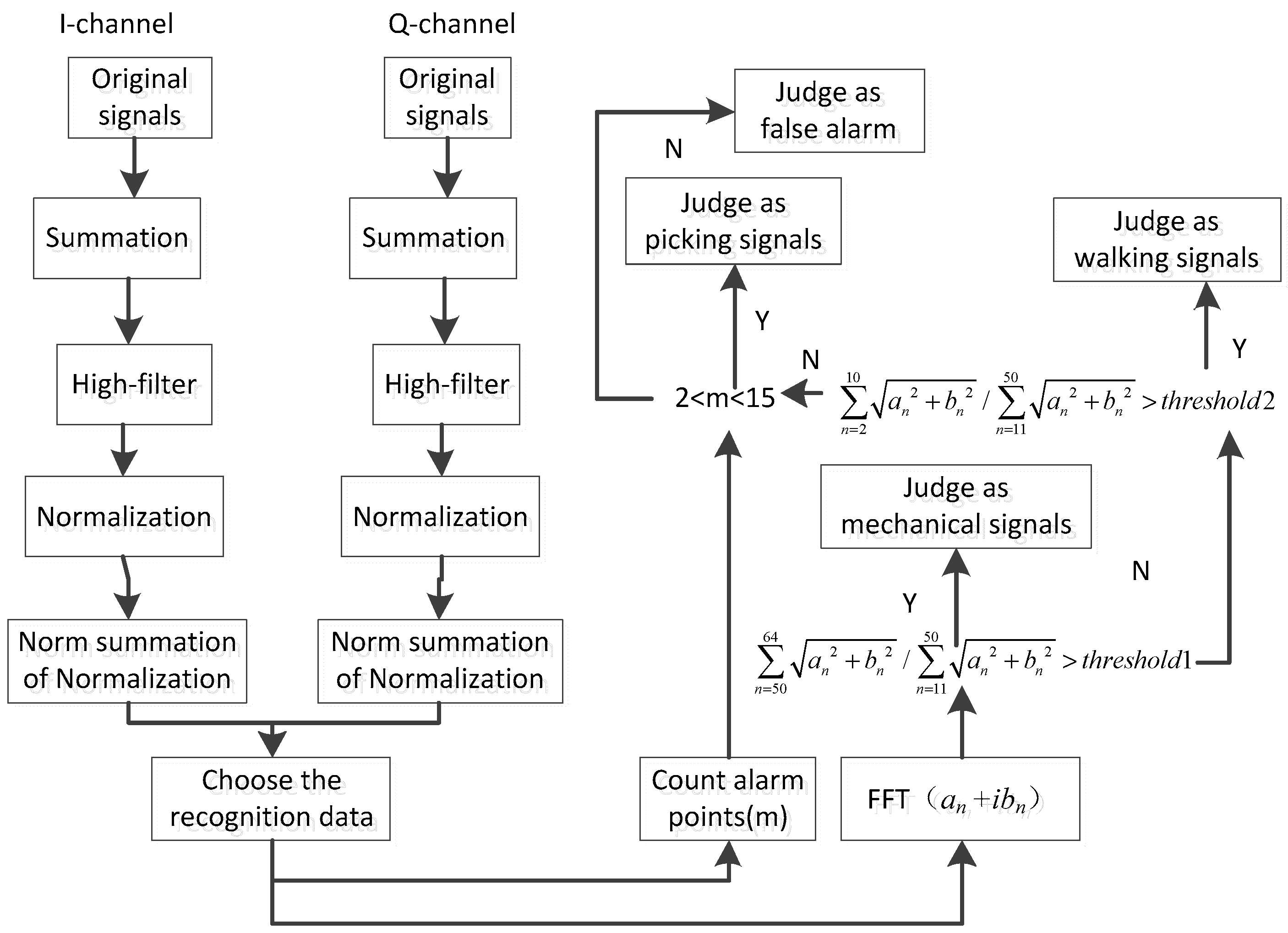
According to the real-time demand of OFPS platform and the characteristics of artificial signal, this paper presents a fast algorithm for the detection and recognition of the optical fiber intrusion signals. The number of operations of this algorithm is , and the number of operations of CFAR algorithm is . The algorithm can be divided into two parts, single-channel detection and recognition. As shown in Figure 1, the collected original data is divided into two paths—I-channel and Q-channel, and the two channels are respectively subjected to summation, high-pass filtering, and then the filtered result is normalized. When the time reaches 1 s, the norm summation of the normalized data of I-channel and Q-channel are obtained. Then, the norm summation of the I-channel and Q-channel is compared, and the larger normalized data are used as the identification data for the next step. The results of the FFT and the number of alarm points are used for identification, and the specific process is described in detail below.
2.1. Single-Channel Detection Algorithm
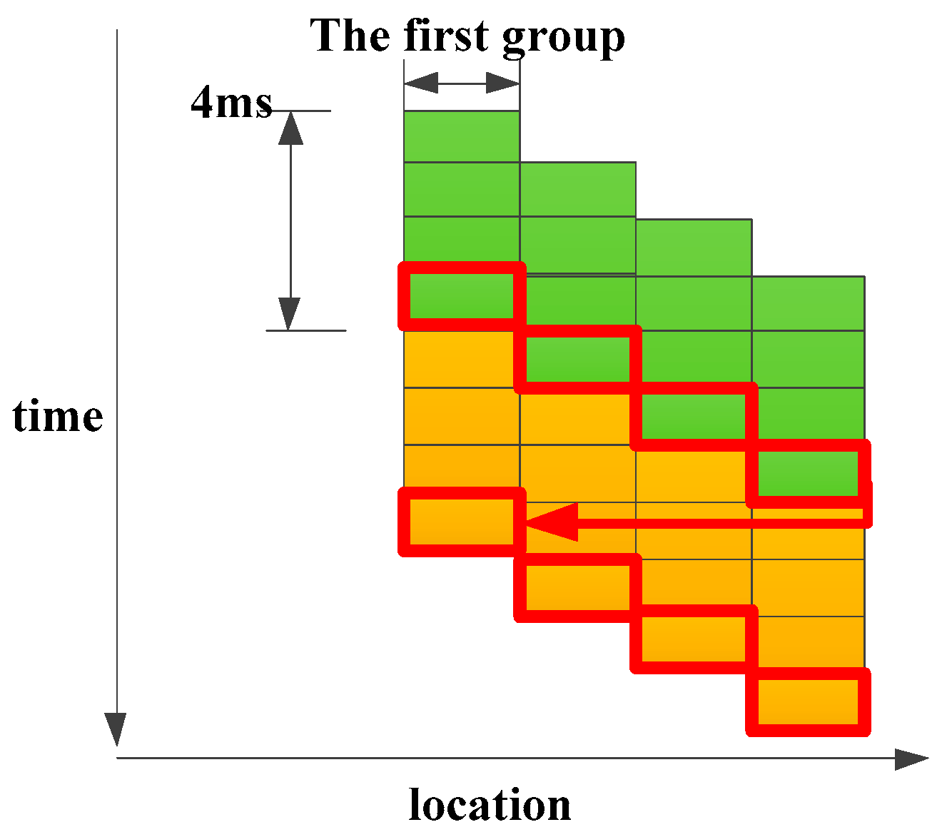
As shown in Figure 2, the original signals are summed adopting the dislocation processing method, and the data is accumulated at a time interval of 4 ms. The total length of the optical cable is 0.72 km. We divide the cable into 45 parts with equal length. Accordingly, the number of the columns is set 45 in our subsequent processing and the length of each column is 16 m. All columns are divided into four groups and the sum value is filtered when the cumulative time reaches 4 ms. As shown in the Figure 3, the number of columns to be filtered in one millisecond is 1/4 of the total columns, and the same processing is performed on the Q-channel data at the same time.
High-pass filtering is performed on the summation results expressed as follows:
where is the current filtering result, is the current summation result, represents the summation result of the previous time unit, represents the filtering result of the last time unit. In addition, , , .
Then the filtered data is normalized as follow
Then the comparison between the normalized data and the threshold is performed.
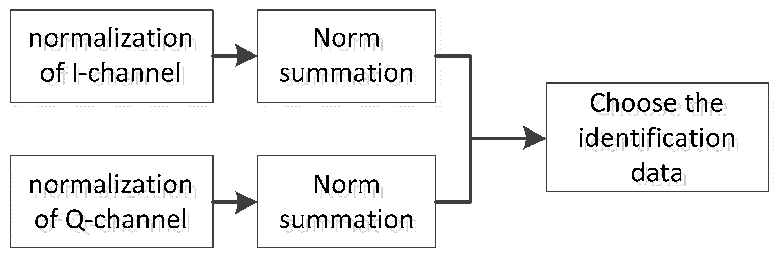
The selection process of the identification data is shown in Figure 4. The norm summation of 128 normalized data points of the I-channel and Q-channel are calculated respectively. Then the two results are compared, and the data with larger norm summation is selected as the identification data.
2.2. Feature Extraction and Identification
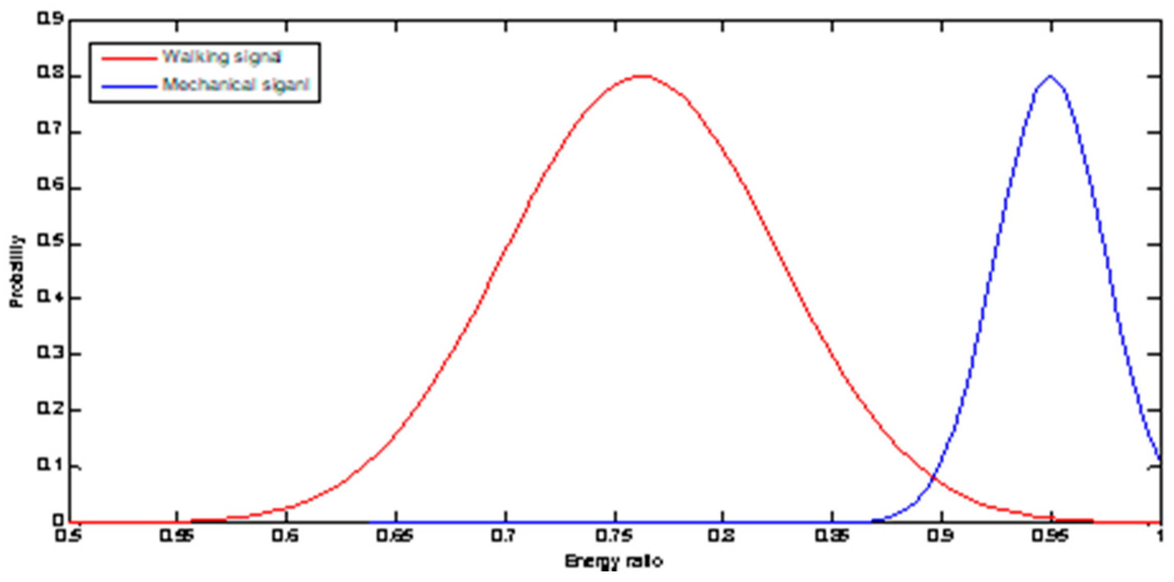
The whole process of feature extraction and identification is shown in Figure 5. The features of OFPS signals are not obvious in the time domain. If these signals are transformed into the frequency domain, the corresponding features are clearer. In addition, FFT can extract the spectrum feature of a signal, which is often used in spectrum analysis. When FFT is performed on N points, the FFT results of N points can be obtained. Because of the symmetry of the FFT results, we usually only use the first half of the results in the frequency domain. The time domain and frequency domain of the data are analyzed, and the following conclusions are obtained: Mechanical signals have a stronger energy between 50 and 64 Hz in the FFT results, while other signals do not have this feature; The walking signal has stronger energy between 2–10 Hz in the FFT result, while other signals do not have this feature; The FFT result of the picking signal does not have obvious features, but its time domain duty cycle is significantly smaller than other signals.
We use a lot of experimental data (or you can edit the number) to find the energy ratio, and fit the obtained result to the probability density function. The probability density function curve is shown in the figure. As can be seen from the figure, thresholds selection is most appropriate at the intersection of the curves.
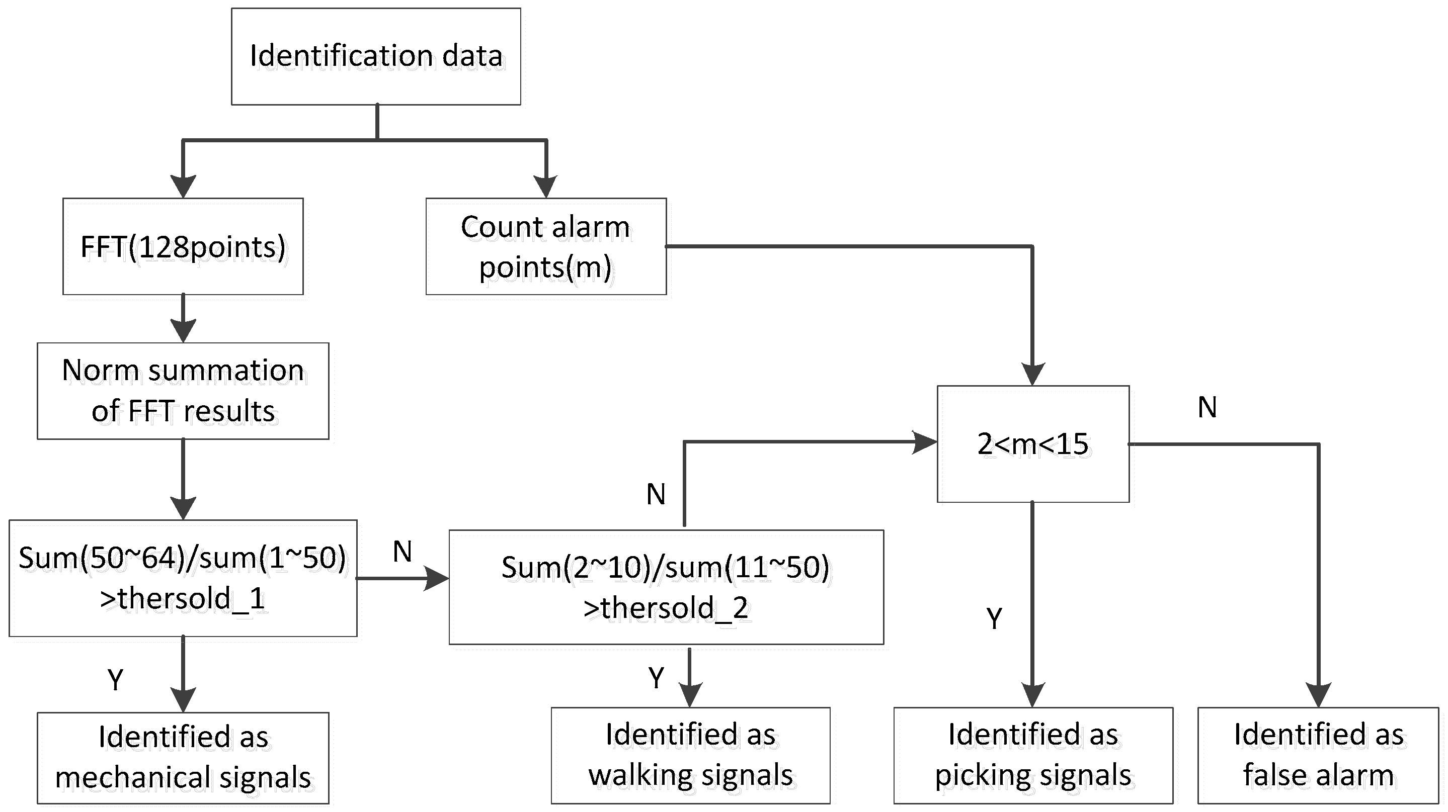
The process of feature extraction and identification is shown in Figure 6. The 128 points FFT is applied for each column of the data. Next, the moduli of points 50–64 and points 11–50 are summed up, respectively. Then the former is divided by the latter and the quotient is compared with the recognition threshold of the mechanical signal. If the quotient is greater than the threshold as shown in Equation (3), where threshold_1 = 0.9, it is judged as mechanical signal.
If the quotient is smaller than the threshold_1, the signal is determined as walking signal. The discrimination method is shown in Equation (4), where threshold_2 = 0.55
If the quotient in Equation (4) is larger than threshold_2, it is judged as walking signal. If the quotient is smaller than threshold_2, the signal will be further identified if it is picking signals.
The picking signal is identified based on the number of alarm points rather than the result of FFT. And if the number of the alarm points is not within the range between 2 and 15, it is ultimately determined as false alarm.
3. The Implementation of Recognition Algorithm and the Experimental Analysis
3.1. The Implementation of Fast Identification Algorithm
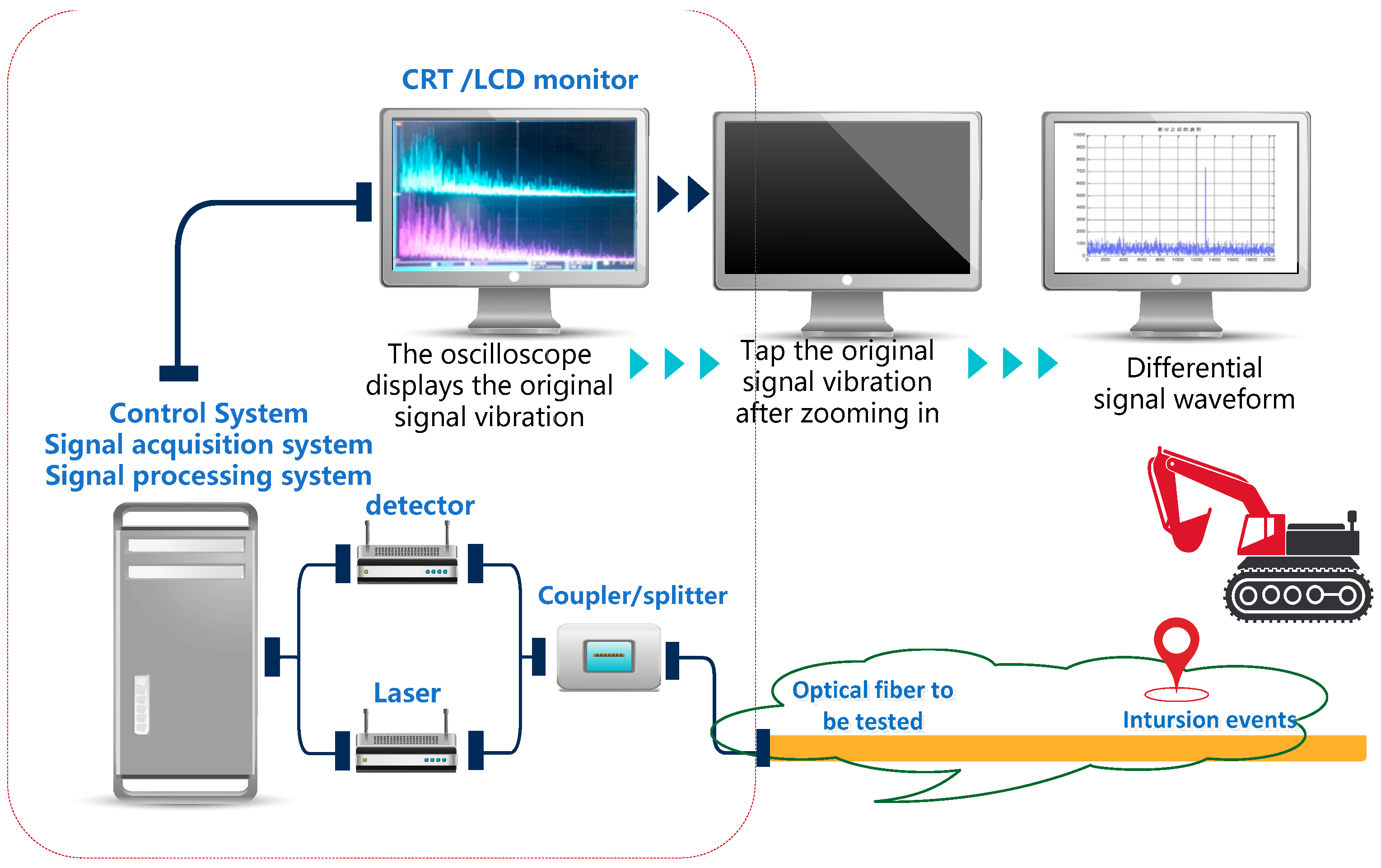
As shown in Figure 7, the optical fiber early warning system is equipped with an optical pulse transmitting board, an optical pulse receiving board, a signal processing board, a data switching board, a motherboard, and a display. Optical pulse-emitting plates are used to modulate, amplify, and emit light pulses. The optical pulse-receiving plate is for receiving backscattered light in the optical fiber and converting the optical signal into an electrical signal. The signal processing board is used to collect and process data, complete the detection and identification of the intrusion signal, and send the alarm result to the upper computer. The software architecture designed in this paper is implemented in the signal processing board. The motherboard runs the host computer software, together with the display to complete the display of the alarm results and the setting of the system parameters.
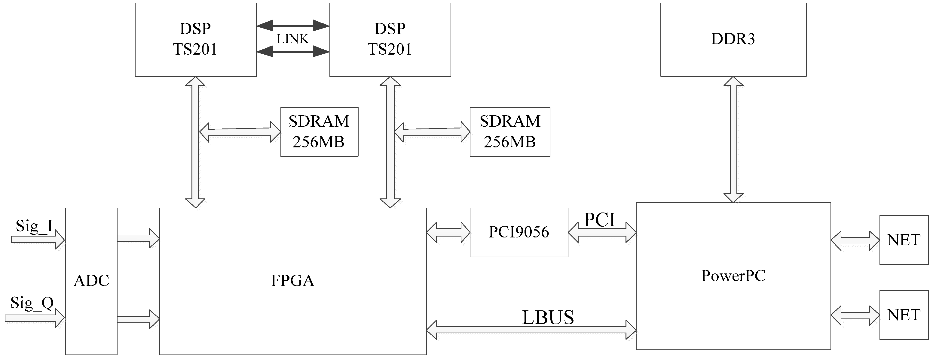
As shown in Figure 8, the fiber-optic warning system signal processing board is equipped with two TS201 processors, one FPGA processor and one PowerPC processor, as well as multiple memory and interface circuits. The signal processing board inputs the in-phase analog signal Sig_I and the quadrature analog signal Sig_Q, and the ADC module with the sampling frequency of 100 MHz is converted into a digital signal; the FIFO queue in the FPGA module is used to read the data in the ADC and cache, and the FPGA takes 1 ms as the the cycle simultaneously initiates an interrupt request to DSP1 and DSP2; DSP1 and DSP2 respond to the interrupt request and read the cache data from the FIFO queue of the FPGA. In addition, the peripheral interface of DSP1 and DSP2 is implemented in the FPGA to ensure data between the two DSPs and the PowerPC. Transparent transmission; PowerPC is responsible for communication with the host computer, and managing DSP software upgrades.
As shown in Figure 9, the entire system is consisted of DSP and host computer. The DSP module is used for optical fiber intrusion signals acquisition at the test site and subsequent signal processing. A mechanical drill is used to shovel the soil near the underground optical fiber, and the mechanical drilling signals are collected. Near the underground optical fiber, electric pick is used to excavate the soil and generate mechanical picking signals. We generate the walking signals by walking around the optical fiber.
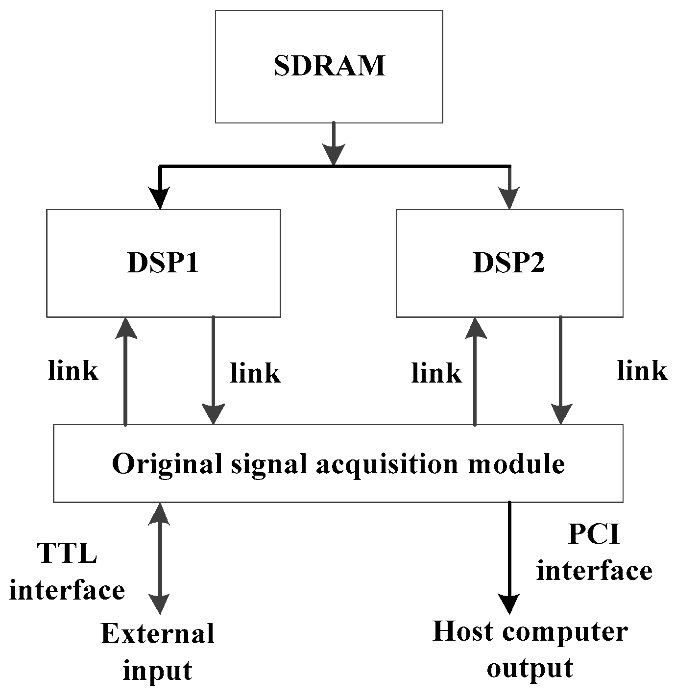
According to the characteristics and requirements of algorithm implementation on embedded hardware, the computational complexity and operation time of each algorithm module are analyzed. The algorithm flow is decomposed into different processors on the board. The processing flow after filtering is distributed in two parallel-processing DSPs. The two DSPs work in parallel and the intermediate results are input to the Synchronous Dynamic Random Access Memory (SDRAM) through the data bus. The external raw data is input to the DSP through the AD interface and LINK port. Finally, the identification results are sent to the host through the PCI interface.
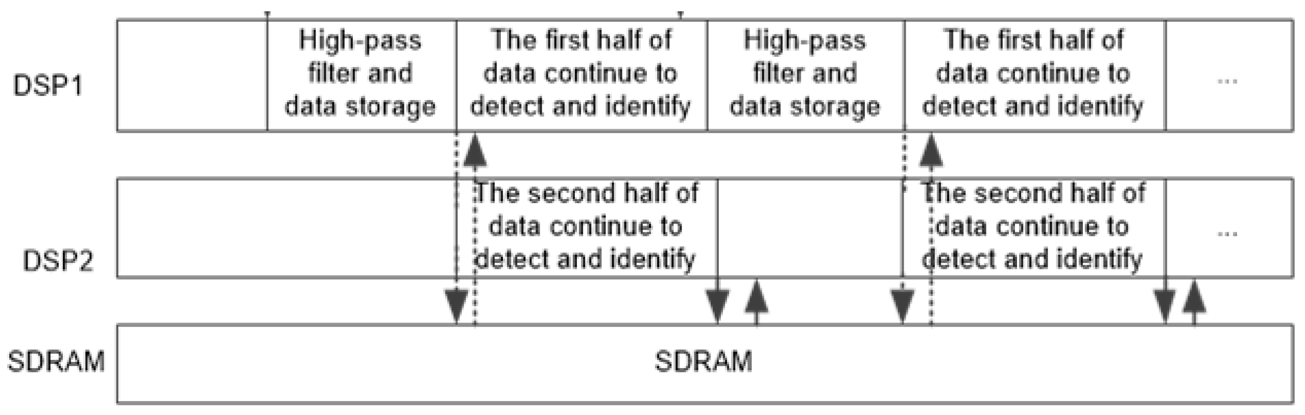
The processing flows in the two DSPs are shown in Figure 10. First, the raw data is received from the TTL interface. Then it is sent to DSP1 through the link port, and stored in the Ping-Pang SDRAM memory. At the same time, DSP1 obtains the data of 1024 ms from the Ping-Pang memory for the subsequent high-pass filtering, and the results are stored in the on-chip RAM. After the detection and identification processing of the first 512 ms filtered data is completed, the results are uploaded through the PCI bus. Then DSP1 waits for the next 1024 ms of data. At the same time, DSP2 obtains the filtered data of the second 512 ms from the Ping-Pang structure for subsequent processing. DSP1 and DSP2 work in parallel mode, and finally determine the output signal type. In this way, parallel flow processing is realized through the Ping-Pang processing of DSP1 and DSP2. The processing time is shortened and the real-time performance is improved.
3.2. Experiment Analysis of Actual Data
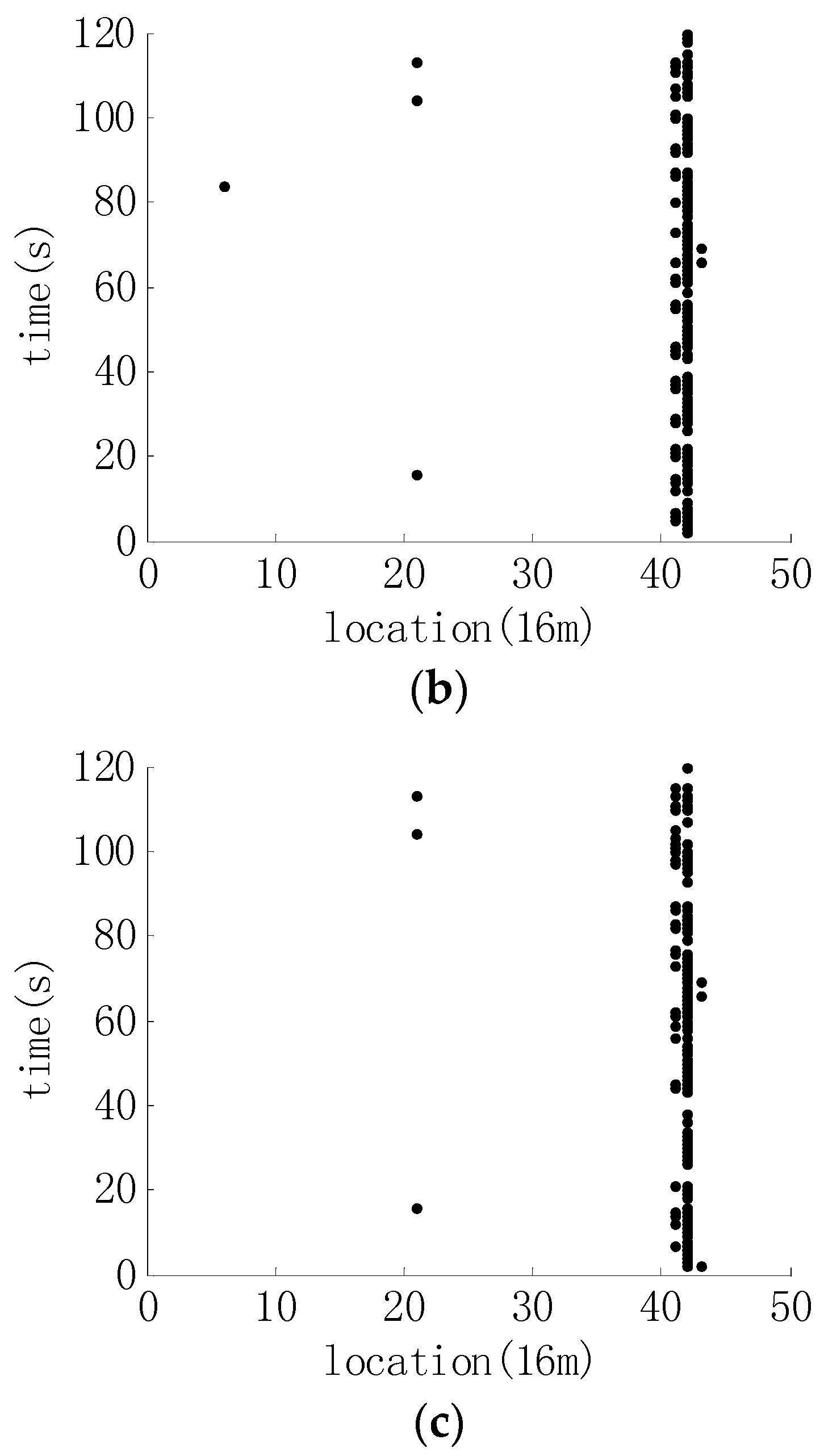
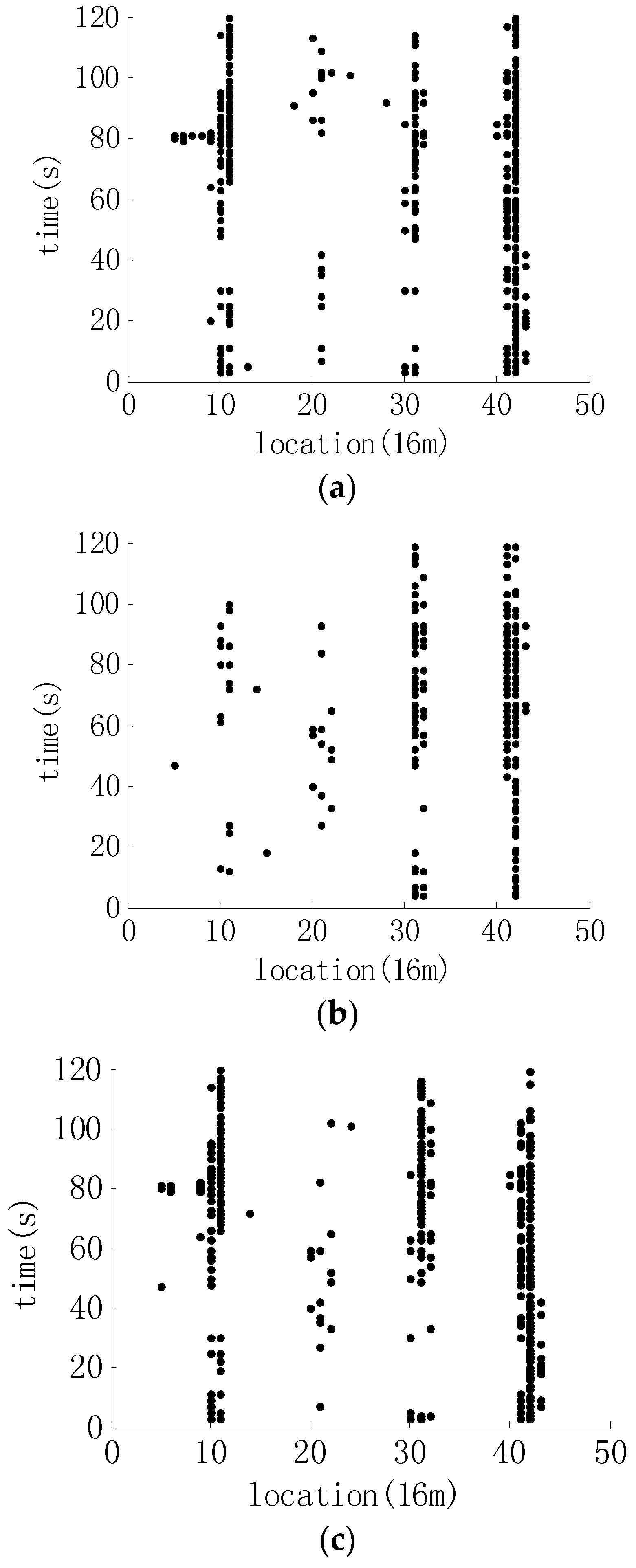
To verify the algorithm, we designed experiments to collect actual data in Shangweidian Village, Mentougou District, Beijing. The tester takes four kinds of actions of mechanical drilling, mechanical picking, walking and picking respectively. Each action is divided into three groups and lasts for 2 min. The size of each group of data is 122,880 rows and 45 columns. In order to observe the detection and identification results, the collection of data is performed in a specific geographical area. It is evident from the results that the signals are mainly concentrated in columns 41 and 42. The abscissa represents the locations and the distance between adjacent columns is 16 m. The ordinate represents time and the unit is second. The number of false alarms is the major factor for the detection. For the identification, the mechanical drilling and mechanical picking signals are both classified as mechanical signals.
3.2.1. The Detection and Identification Results of Mechanical Signals
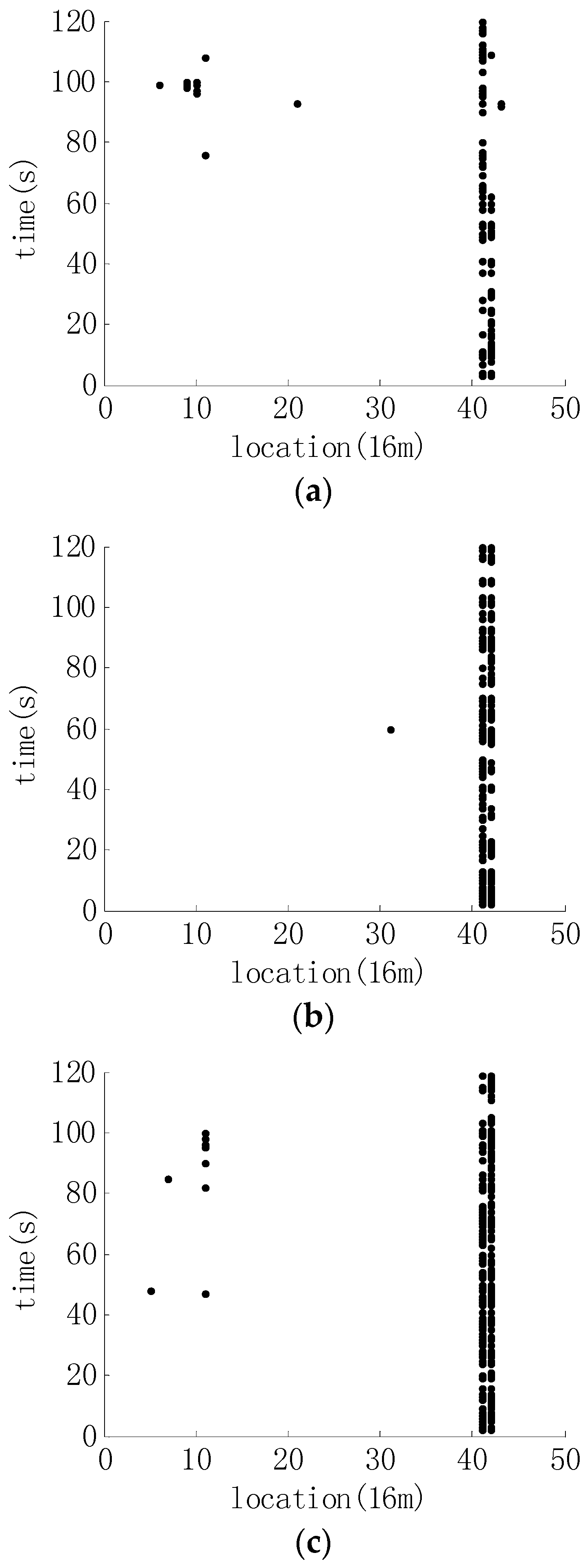
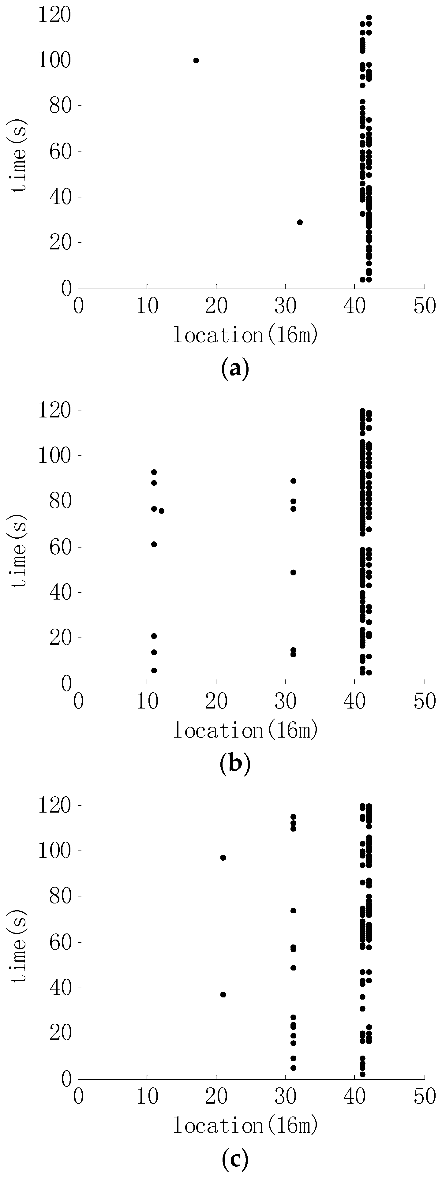
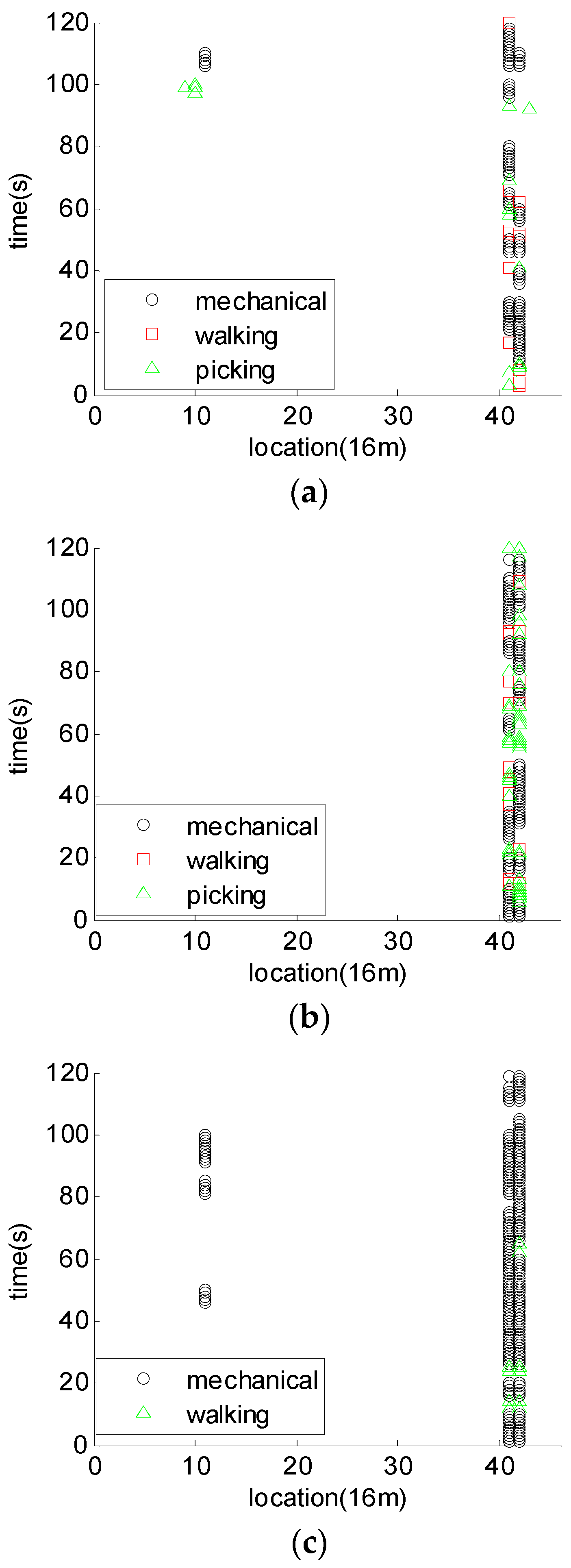
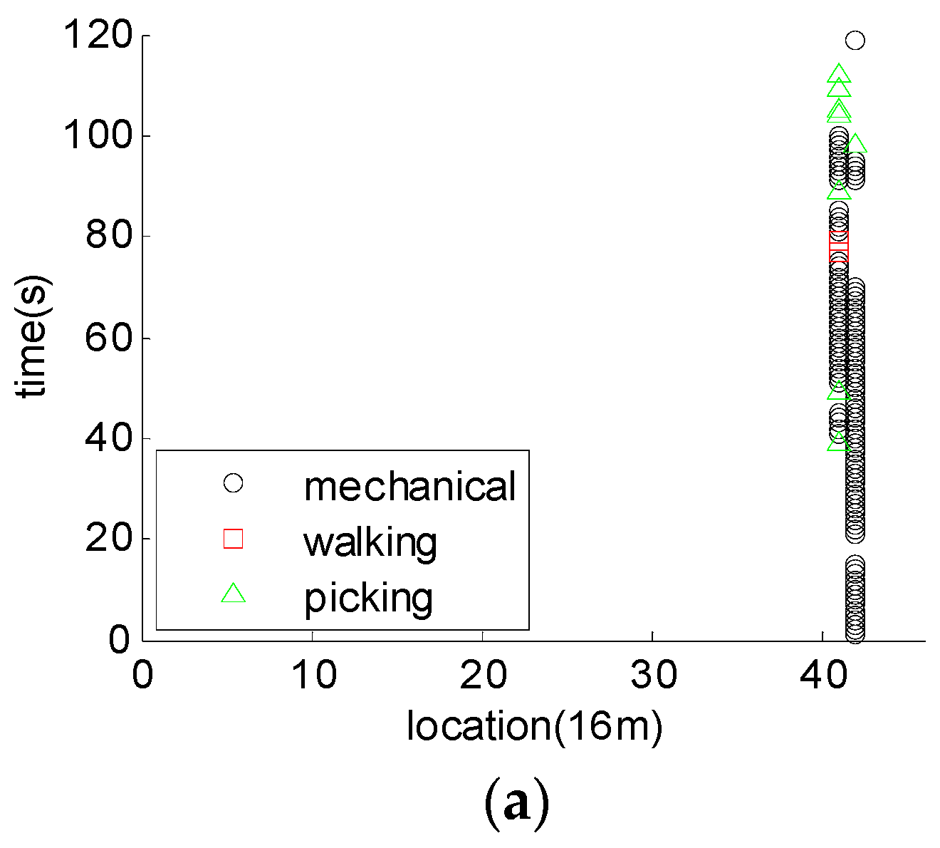
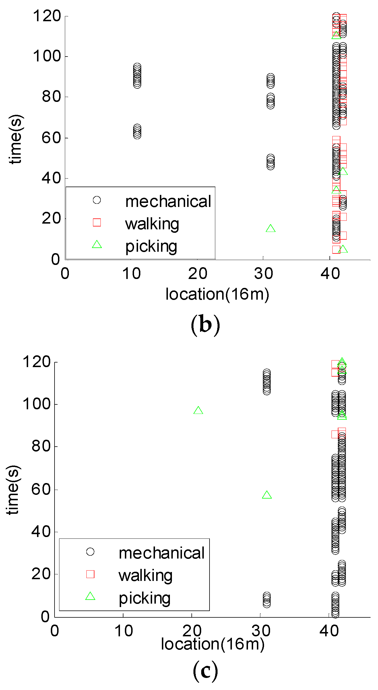
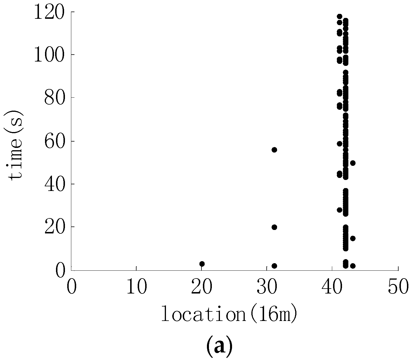
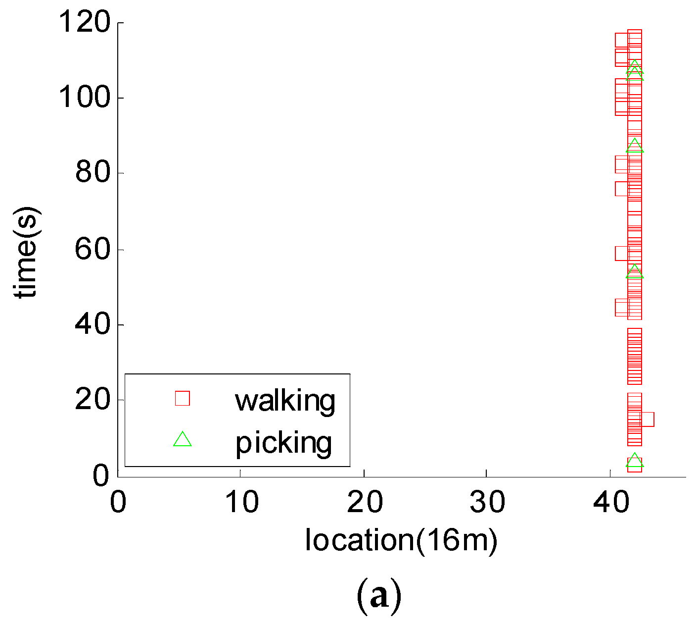
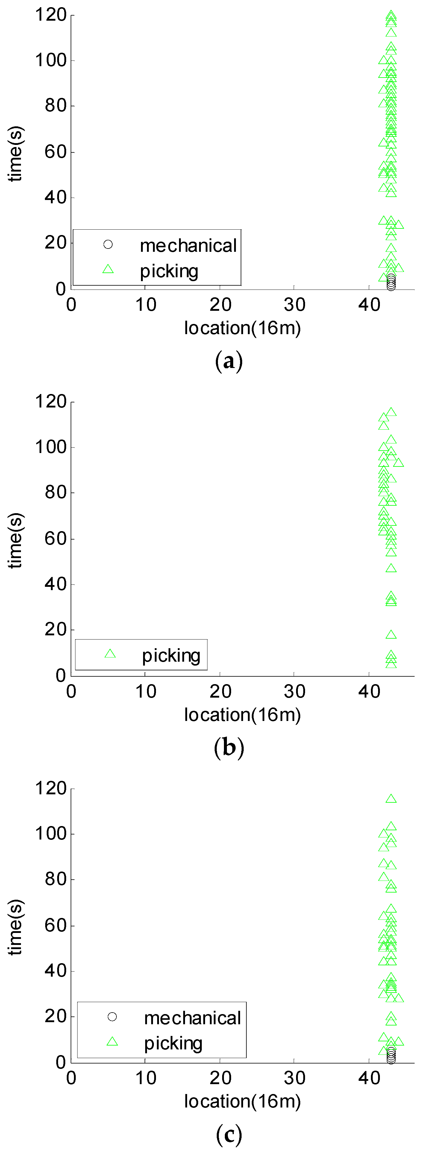
In the figures of detection results, the black dots represent the optical fiber vibration signals. FFT is applied to the identification data extracted from the detection results, and the sum of the FFT results of different frequency bands is compared with the recognition threshold. The intrusion type of signals is judged as the identification result. In the figures of the identification results, black circles represent mechanical signals, red squares represent walking signals, and green triangles represent picking signals.
It can be observed from Figure 11 and Figure 12 that the alarms of the mechanical signals are mainly concentrated in the 41st column and 42nd column. There are only a few false alarm points near the 10th column and 11th column. Overall, the detection results are relatively ideal. And in the subsequent identification processing, the alarm point will be further verified.
The statistical recognition result of mechanical drilling is shown in Table 1. The drill 1, drill 2 and drill 3 at the Table 1 represent three groups of mechanical drilling signals. The picking, mechanical and walking in the first row of Table 1 represent the number of the signals which are finally recognized as these three types. The statistics method for recognition rate of following three types of signals is the same as the mechanical drilling signals. The recognition result of mechanical drilling signals is shown in figures above. The ratio of the number of each kind of signal to the total number is calculated, respectively, and the recognition rate is obtained. The statistical recognition rate is shown in Table 2.
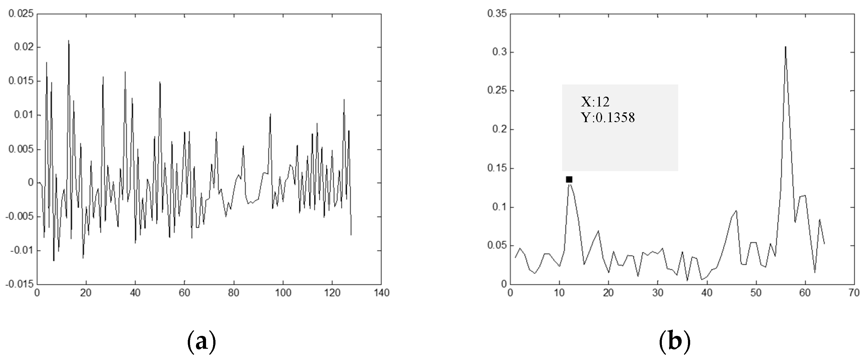
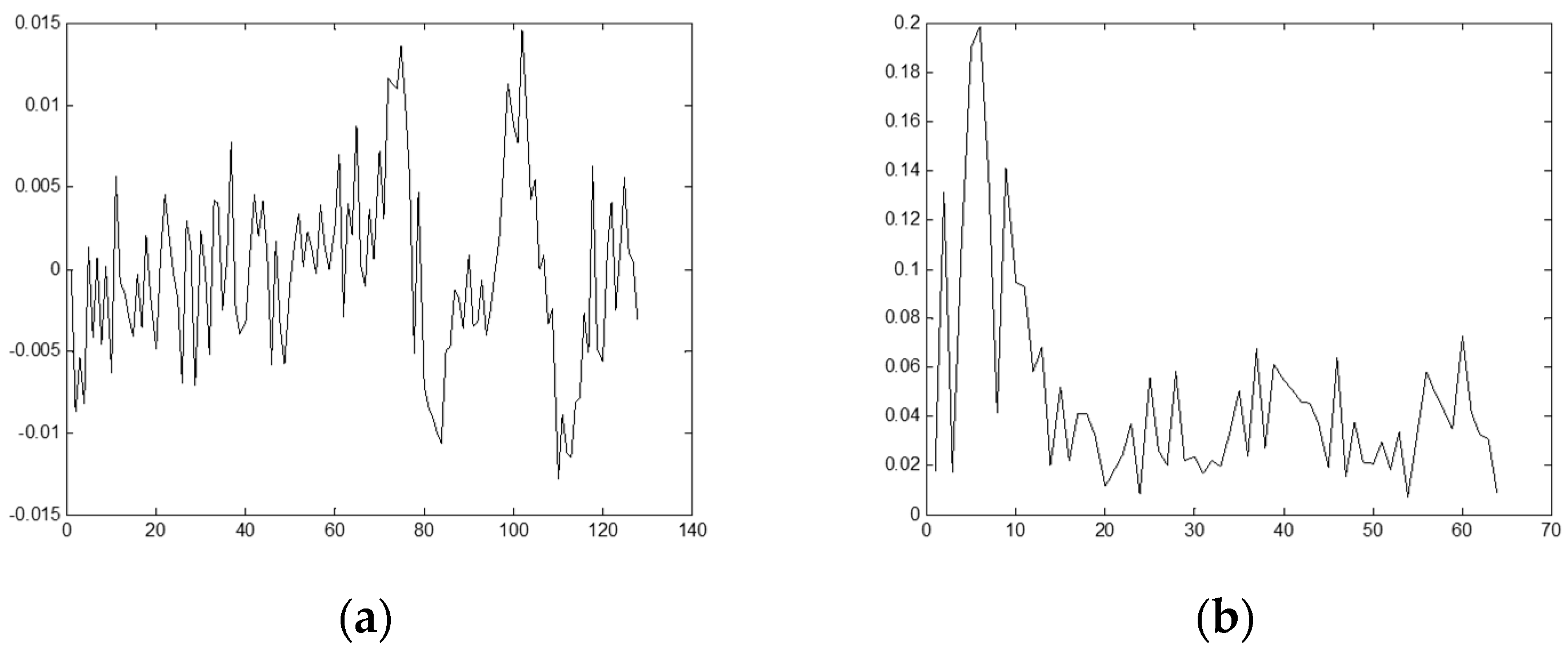
As shown in Figure 15, the reason why the mechanical drilling signal is recognized as picking signal is that the feature extracted by FFT has strong energy from 50 Hz to 64 Hz, but there is an obvious peak value at 12 Hz resulting in a small ratio of 0.7737 much below the threshold. As shown in Figure 16, the reason why the mechanical drilling signal is recognized as walking signal is that the characteristics of mechanical drilling are not obvious where there is no remarkable high frequency component and the low frequency component is large.
3.2.2. The Detection and Identification Results of Walking Signals
The detection results of walking signals are as Figure 17:
The alarm points of the walking signals are mainly concentrated in the 41st column and 42nd column, which is the location of the collected data. The false alarm point is relatively the least among these four types of signals.
The identification results of walking signals are shown in Figure 18:
As shown in Table 3, the recognition rate of the walking signals is very high, and there are no walking signals recognized as mechanical signals. In a few cases, walking signal is recognized as picking signal. As shown in Figure 19, the walking signals’ features extracted by FFT have no obvious peak value in the range of 2–10 Hz. The ratio calculated in this part is 0.3421, which is far below the threshold 0.55, so it will not be judged as walking signal. At the same time, the number of alarm points which belongs to this second is 7, which is also in the range of 2–15, so it is judged as a picking signal.
3.2.3. The Identification Results of Picking Signals
The detection results of picking signals are as Figure 20:
The noise signal is different from the previous two types of signals. The alarm points are not only concentrated in the 41st and 42th columns. The alarm points in the 10th, 11th, and 31st columns are also very obvious. However, it does not mean that the 10th column, 11th column, and 31th column are vibration signals. And in the subsequent identification processing, the alarm point will be further verified.
The identification results of picking signals are shown in Figure 21:
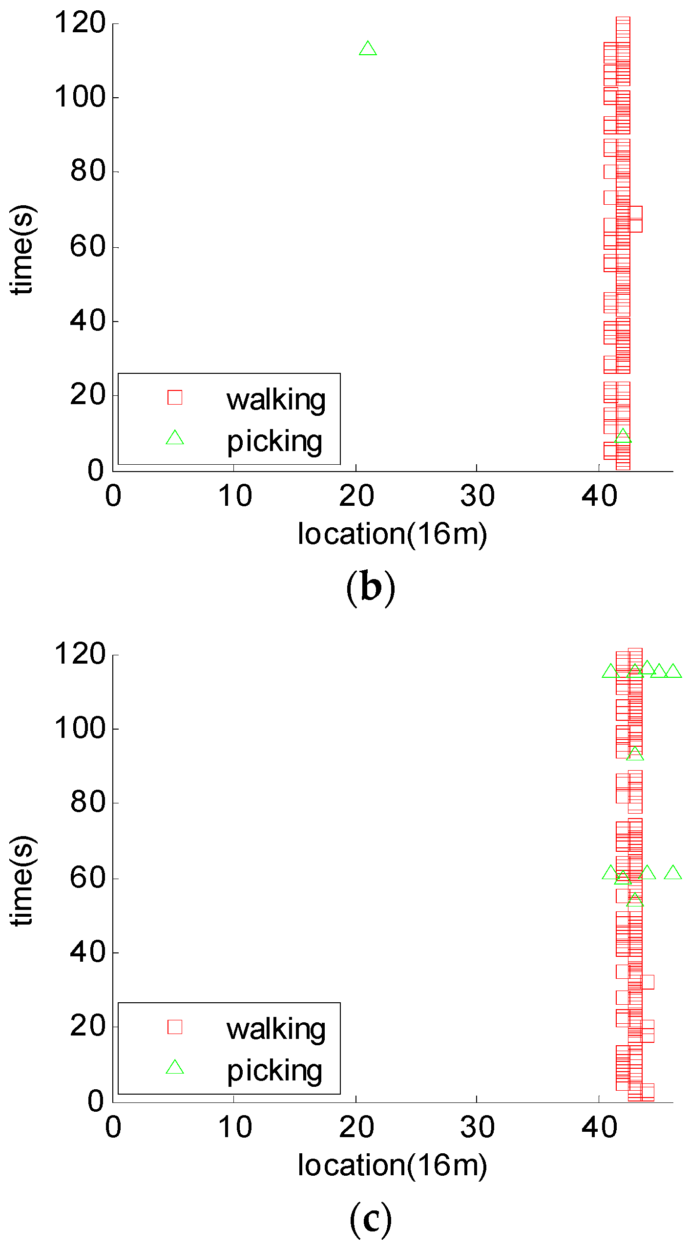
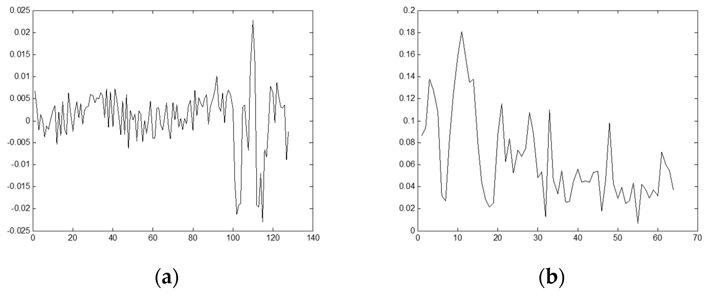
As shown in Table 4, the recognition rate of picking signals is almost completely right. The recognition of one group of data is 100%, and the other group is 0.9618. A very few of picking signals are recognized as mechanical signals. It is shown in Figure 22 that the low frequency component of picking signal is obvious and the ratio is 0.7223, which is obviously larger than the threshold value, 0.55, so it is judged as a mechanical signal.
3.2.4. The Performance Comparison of Fast Algorithm with Other Methods
As shown in Table 5, the false alarm rate of single-channel detection algorithm proposed in this article is 2.6% lower than Cell Average Constant False Alarm Rate (CA-CFAR).
The recognition performance of each method is shown in Table 6. The recognition rate of the methods used in this paper is relatively high, and the average recognition rate is 93.51%.
The real-time performance of each method is shown in Table 7 that is better than other strategies with the time consumption of 0.659 s. It can be seen that the method adopted in this paper not only guarantees the recognition rate, but also is superior to other algorithm in time efficiency.
4. Conclusions
In recent years, the research on detection and identification algorithms of optical fiber vibration signals has made great progress. Scholars have proposed many algorithms and strategies, but most of them are in the simulation stage. Based on this, this paper presents a fast detection and identification algorithm for optical fiber intrusion signals that can be implemented on embedded platforms. The algorithm has been implemented on a DSP-based hardware board and actually tested the algorithm in Mentougou District, Beijing. Several common intrusion vibration signals are detected and identified. The results show that the detection performance is good, and the average recognition rate is above 90%. The threshold training of this algorithm is pre-processed on the personal computer (PC) side, so it saves a lot of time when implemented on the embedded platform, and the application of the parallel method can further increase the running speed. The specific time consumption is 0.659 s, which proves the effectiveness of the algorithm proposed in this paper.
Author Contributions
Conceptualization, Z.S. and Y.Z.; Methodology, Z.S.; Software, D.Y.; Validation, D.Q. and Y.Z.; Formal Analysis, D.Q.; Investigation, Y.Z.; Resources, D.Q.; Data Curation, D.Y.; Writing-Original Draft Preparation, D.Q.; Writing-Review & Editing, D.Q.; Visualization, Z.S.; Supervision, Y.Z.; Project Administration, Y.Z.; Funding Acquisition, Y.Z.
Funding
This research was funded by [the National Natural Science Foundation of China] grant number [61571014 and 61601006].
Acknowledgments
The authors wish to express their gratitude to the anonymous reviewers and the associate editor for their rigorous comments during the review process. In addition, authors also would like to thank experimenters in our laboratory for their great contribution on data-collection work. They are Sun Chengbin, Tan Lei, Feng Tingliang. This work was supported by the National key R&D Program Project [grant No. 2017YFB1201104].
Conflicts of Interest
The authors declare no conflict of interest.
References
- Liu, K.; Chai, T.J.; Liu, T.G.; Jiang, J.F.; Chen, Q.N.; Pan, L. Multi-area optical perimeter security system with quick invasion judgement algorithm. J. Optoelectron. Laser 2015, 26, 288–294. (In Chinese) [Google Scholar]
- Jing, K.; Zhi-Hong, Z. Time prediction model for pipeline leakage based on grey relational analysis. Phys. Procedia 2010, 25, 2019–2024. [Google Scholar] [CrossRef]
- Liang, W.; Lu, L.; Zhang, L. Coupling relations and early-warning for ‘equipment chain’ in long-distance pipeling. Mech. Syst. Signal Process. 2013, 41, 335–347. [Google Scholar] [CrossRef]
- Liang, W.; Zhang, L.; Xu, Q.; Yan, C. Gas pipeline leakage detection based on acoustic technology. Eng. Fail. Anal. 2013, 31, 1–7. [Google Scholar] [CrossRef]
- Zhang, T.; Tan, Y.; Yang, H.; Zhao, J.; Zhang, X. Locating gas pipeline leakage based on stimulus-response method. Energy Procedia 2014, 61, 207–210. [Google Scholar] [CrossRef]
- Zhu, C.H.; Qu, Y.Z.; Wang, J.P. The vibration signal recognition of optical fiber perimeter based on time-frequency features. Opto-Electron. Eng. 2014, 41, 16–22. [Google Scholar]
- Qu, H.; Zheng, T.; Pang, L.; Li, X. A new detection and recognition method for optical fiber pre-warning system. Optik 2017, 137, 209–219. [Google Scholar] [CrossRef]
- Zhang, R.; Sheng, W.; Ma, X. Improved switching CFAR detector for non-homogeneous environments. Signal Process. 2013, 93, 35–48. [Google Scholar] [CrossRef]
- Weinberg, G.V. Management of interference in Pareto CFAR processes using adaptive test cell analysis. Signal Process. 2014, 104, 264–273. [Google Scholar] [CrossRef]
- Shi, B.; Hao, C.; Hou, C.; Ma, X.; Peng, C. Parametric Rao test for multichannel adaptive detection of range-spread target in partially homogeneous environments. Signal Process. 2015, 108, 421–429. [Google Scholar] [CrossRef]
- Tao, P.; Yan, F.; Liu, P.; Peng, W.; Li, Q.; Feng, T. Fiber-optic intrusion recognition system based on Mach-Zehnder interferometer. Chin. J. Quantum Electron. 2011, 28, 183–190. [Google Scholar]
- Wang, S. M-Z interferometer Optical Fiber Sensing System of distributed disturbance pattern recognition method. Infrared Laser Eng. 2014, 43, 613–618. [Google Scholar]
- Qu, H.; Ren, X.; Li, G.; Li, Y.; Zhang, C. Study on the algorithm of vibration source identification based on the optical fiber vibration pre-warning system. Photonic Sens. 2015, 5, 180–188. [Google Scholar] [CrossRef] [Green Version]
- Qu, H.; Liu, S.; Wang, Y.; Li, G. Approach to identifying raindrop vibration signal detected by optical fiber. Sens. Transducers 2013, 160, 85–92. [Google Scholar]
- Qin, Z.; Chen, L.; Bao, X. Continuous wavelet transform for non-stationary vibration detection with phase-OTDR. Opt. Express 2012, 20, 20459–20465. [Google Scholar] [CrossRef] [PubMed]
- Hui, X.; Zheng, S.; Zhou, J.; Chi, H.; Jin, X.; Zhang, X. Hilbert-Huang Transform Time-Frequency Analysis in phi-OTDR Distributed Sensor. IEEE Photonics Technol. Lett. 2014, 26, 2403–2406. [Google Scholar] [CrossRef]
- Zhu, C.; Zhao, Y.; Wang, J.; Li, W.; Zhang, Q. Ensemble Recognition of Fiber Intrusion Behavior Based on Blending Features. Opto-Electron. Eng. 2016, 43, 6–12. [Google Scholar]
Figure 1.
The whole flow of the algorithm.

Figure 2.
Flow of single–channel detection.

Figure 3.
Summation of every 4 ms in I-channel.

Figure 4.
Extraction of identification data.

Figure 5.
Feature extraction and identification.

Figure 6.
The selection processing of thresholds.

Figure 7.
Optical fiber Pre-warning monitoring system.

Figure 8.
Signal processing board module diagram.

Figure 9.
Frame diagram of hardware implementation.

Figure 10.
Structure diagram of parallel processing.

Figure 11.
The detection results of mechanical drilling signals. (a) The first group of mechanical drilling signals; (b) The second group of mechanical drilling signals; (c) The third group of mechanical drilling signals.
Figure 11.
The detection results of mechanical drilling signals. (a) The first group of mechanical drilling signals; (b) The second group of mechanical drilling signals; (c) The third group of mechanical drilling signals.

Figure 12.
The detection results of mechanical picking signals. (a) The first group of mechanical picking signals; (b) The second group of mechanical picking signals; (c) The third group of mechanical picking signals.
Figure 12.
The detection results of mechanical picking signals. (a) The first group of mechanical picking signals; (b) The second group of mechanical picking signals; (c) The third group of mechanical picking signals.

Figure 13.
The identification results of mechanical drilling signals. (a) The first group of mechanical drilling signals; (b) The second group of mechanical drilling signals; (c) The third group of mechanical drilling signals.
Figure 13.
The identification results of mechanical drilling signals. (a) The first group of mechanical drilling signals; (b) The second group of mechanical drilling signals; (c) The third group of mechanical drilling signals.

Figure 14.
The identification results of mechanical picking signals. (a) The first group of mechanical picking signals; (b) The second group of mechanical picking signals; (c) The third group of mechanical picking signals.
Figure 14.
The identification results of mechanical picking signals. (a) The first group of mechanical picking signals; (b) The second group of mechanical picking signals; (c) The third group of mechanical picking signals.


Figure 15.
Mechanical signal recognized as picking signal. (a) Time domain; (b) Frequency domain.

Figure 16.
Mechanical drilling signal recognized as walking signal. (a) Time domain; (b) Frequency domain.
Figure 16.
Mechanical drilling signal recognized as walking signal. (a) Time domain; (b) Frequency domain.

Figure 17.
The detection results of walking signals. (a) The first group of walking signals; (b) The second group of walking signals; (c) The thrid group of walking signals.
Figure 17.
The detection results of walking signals. (a) The first group of walking signals; (b) The second group of walking signals; (c) The thrid group of walking signals.


Figure 18.
The identification results of walking signals. (a) The first group of walking signals; (b) The second group of walking signals; (c) The third group of walking signals.
Figure 18.
The identification results of walking signals. (a) The first group of walking signals; (b) The second group of walking signals; (c) The third group of walking signals.


Figure 19.
Walking signal recognized as picking signal. (a) Time domain; (b) Frequency domain;

Figure 20.
The detection results of picking signals. (a) The first group of picking signals; (b) The second group of picking signals; (c) The third group of picking signals.
Figure 20.
The detection results of picking signals. (a) The first group of picking signals; (b) The second group of picking signals; (c) The third group of picking signals.

Figure 21.
The identification results of picking signals. (a) The first group of picking signals; (b) The second group of picking signals; (c) The third group of picking signals.
Figure 21.
The identification results of picking signals. (a) The first group of picking signals; (b) The second group of picking signals; (c) The third group of picking signals.

Figure 22.
Picking signal recognized as walking signal. (a) Time domain; (b) Frequency domain;


Table 1.
The statistical identification results of Mechanical drilling signals.
| Picking | Mechanical | Walking | |
|---|---|---|---|
| Mechanical drilling1 | 14 | 93 | 8 |
| Mechanical drilling2 | 30 | 107 | 10 |
| Mechanical drilling3 | 0 | 210 | 10 |
Table 2.
The identification rate of Mechanical signals.
| Picking | Mechanical | Walking | |
|---|---|---|---|
| Mechanical drilling1 | 12.1% | 80.9% | 7.0% |
| Mechanical drilling2 | 20.4% | 72.8% | 6.8% |
| Mechanical drilling3 | 0 | 95.5% | 4.5% |
| Mechanical picking1 | 6.3% | 92.1% | 1.6% |
| Mechanical picking2 | 10.4% | 86.5% | 3.1% |
| Mechanical picking3 | 4.5% | 91.6% | 3.9% |
Table 3.
The identification rate of walking signals.
| Mechanical | Walking | Picking | |
|---|---|---|---|
| walking 1 | 5.6% | 94.4% | 0 |
| walking 2 | 1.6% | 98.4% | 0 |
| walking 3 | 2.7% | 97.3% | 0 |
Table 4.
The identification rate of picking signals.
| Picking | Mechanical | Walking | |
|---|---|---|---|
| Picking 1 | 96.2% | 3.8% | 0 |
| Picking 2 | 100% | 0 | 0 |
| Picking 3 | 95.6% | 4.4% | 0 |
Table 5.
Comparison of detection performance of single-channel detection algorithm with CA-CFAR.
| Method | False Alarm Rate | Realization Method |
|---|---|---|
| single-channel detection algorithm | 5.2% | Embedded platform |
| CA-CFAR | 7.8% | Embedded platform |
© 2018 by the authors. Licensee MDPI, Basel, Switzerland. This article is an open access article distributed under the terms and conditions of the Creative Commons Attribution (CC BY) license (http://creativecommons.org/licenses/by/4.0/).
Share and Cite
MDPI and ACS Style
Sheng, Z.; Qu, D.; Zhang, Y.; Yang, D. The Fast Detection and Identification Algorithm of Optical Fiber Intrusion Signals. Algorithms 2018, 11, 129. https://doi.org/10.3390/a11090129
AMA Style
Sheng Z, Qu D, Zhang Y, Yang D. The Fast Detection and Identification Algorithm of Optical Fiber Intrusion Signals. Algorithms. 2018; 11(9):129. https://doi.org/10.3390/a11090129
Chicago/Turabian StyleSheng, Zhiyong, Dandan Qu, Yuan Zhang, and Dan Yang. 2018. "The Fast Detection and Identification Algorithm of Optical Fiber Intrusion Signals" Algorithms 11, no. 9: 129. https://doi.org/10.3390/a11090129
Note that from the first issue of 2016, this journal uses article numbers instead of page numbers. See further details here.