A QUBO Model for the Traveling Salesman Problem with Time Windows

Abstract

This work focuses on expressing the TSP with Time Windows (TSPTW for short) as a quadratic unconstrained binary optimization (QUBO) problem. The time windows impose time constraints that a feasible solution must satisfy. These take the form of inequality constraints, which are known to be particularly difficult to articulate within the QUBO framework. This is, we believe, the first time this major obstacle is overcome and the TSPTW is cast in the QUBO formulation. We have every reason to anticipate that this development will lead to the actual execution of small scale TSPTW instances on the D-Wave platform.

1. Introduction

Quantum computing promotes the exploit of quantum-mechanical principles for computation purposes. Richard Feynman in 1982 suggested that computation could be done more efficiently by taking advantage of the power of quantum “parallelism” [1]. Since then, quantum computing has gained a lot of momentum and today appears to be one of the most prominent candidates to partially replace classical, silicon-based systems. There exist a number of quantum algorithms that run more efficiently than the best known classical counterparts; arguably, the most famous ones are Shor’s [2] and Grover’s [3] algorithms. For an in-depth study of quantum computing and quantum information, the reader is referred to [4].

Adiabatic quantum computation was proposed by Farhi et al. [5,6] in the early 2000s [7]. It is based on an important theorem of quantum mechanics, the adiabatic theorem [8,9]. This theorem asserts that if a quantum system is driven by a slowly changing Hamiltonian that evolves from $H_{init}$ to $H_{fin}$, then if the systems starts in the ground state of $H_{init}$, the system will end up in the ground state of $H_{fin}$. It has been shown that adiabatic quantum computation is equivalent to standard quantum computation [10].

Quantum annealing is based on the quantum adiabatic computation paradigm. Quantum annealing was initially proposed by Kadowaki and Nishimori [11,12] and has since then been used for tackling combinatorial optimization problems. The way that a quantum annealer tries to solve problems is very similar to the way optimization problem are solved using (classical) simulated annealing [13]. An energy landscape is constructed via a multivariate function, such that the ground state corresponds to the solution of the problem. The quantum annealing process is iterated until an optimal solution is found with a sufficiently high probability. The “quantum” in “quantum annealer” refers to the use of multi qubit tunneling [11,12]. The high degree of parallelism is the advantage of quantum annealing over classical code execution. A quantum annealer explores all possible inputs in parallel to find the optimal solution to a problem, which might prove crucial when it comes to solving NP-complete problems. We caution the reader however that, at present, these techniques should be considered more as an automatic heuristic-finding program than as a formal solver [14].

The prospect of employing quantum computing principles for solving optimization problems is particularly promising [15,16,17,18,19]. In this approach, which can be considered as an “analog” method to tackle optimization problems, the ground state of a Hamiltonian represents an optimal solution of the optimization problem at hand. Typically, the quantum annealing process starts with the system being in an equal superposition of all states. Then, an appropriate Hamiltonian is applied and the system evolves in a time-dependent manner according to the Schrödinger equation. The state of the system keeps changing according to strength of the local transverse field, which varies with respect to time. Finally, the transverse field is smoothly turned off and the system finds itself in the ground state of a properly chosen Hamiltonian that encodes an optimal solution of the optimization problem.

The D-Wave platform, the first actual commercial system based upon quantum annealing, has demonstrated its ability to solve certain quadratic unconstrained (mainly binary) optimization problems. The core of D-Wave’s machine that applies the quantum annealing principles for complex combinatorial optimization problems is the quantum processing unit (QPU). In the D-Wave computer, the quantum bits (which we refer to as qubits from now on) are the lowest energy states of superconducting loops [7,20,21]. In these states, there is a circulating current and a corresponding magnetic field. Since a qubit is a quantum object, its state can be a superposition of the 0 state and the 1 state at the same time. However, upon measurement, a qubit collapses to the state 0 or 1 and behaves as a classical bit. The quantum annealing process in effect guides the qubits from a superposition of states to their collapse into either the 0 or 1 state. In the end, the net effect is that the system is in a classical state, which must encode an (optimal) solution of the problem.

The current generation of D-Wave computers employs the Chimera topology. In the Chimera topology, qubits are sets of connected unit cells that are connected to four vertical qubits via couplers [21,22,23]. The unit cells are oriented vertically and horizontally with adjacent qubits connected, creating a sparsely connected network. A Chimera graph consists of an $N\times N$ grid of unit cells. The D-Wave 2000Q QPU has up to 2048 qubits, which are mapped to a C16 Chimera graph, that is they are logically mapped into a $16\times 16$ matrix of unit cells, each consisting of 8 qubits. In the D-Wave nomenclature the percentage of working qubits and couplers is known as the working graph, which is typically a subgraph of the total number of interconnected qubits that are physically present in the QPU.

A major category of optimization problems, particularly amenable to D-Wave’s quantum annealing, are those that can be expressed as quadratic unconstrained binary optimization (QUBO) problems. QUBO refers to a pattern matching technique that, among other applications, can be used in machine learning and optimization, and which involves minimizing a quadratic polynomial over binary variables [21,24,25,26,27,28,29,30]. We emphasize that QUBO is NP-hard [30]. Some of the most famous combinatorial optimization problems that can be solved as QUBO problems are the Maximum Cut, the Graph Coloring and the Partition problem [31]. More details on the QUBO formulation and related results (that are beyond the scope of this paper) can be found in the survey paper of Kochenberger [26]. QUBO is equivalent to the Ising model, a well-known and extensively studied model in physics, that was introduced in the mid-1920s by Ernst Ising and Wilhelm Lenz in the field of ferromagnetism [32,33]. The underlying logical architecture of this model is that variables are represented as qubits and interactions among qubits stand for the costs associated with each pair of qubits. In particular, this architecture can be depicted as an undirected graph with qubits as vertices and couplers as edges among them. The open-source software qbsolv that D-Wave introduced in 2017 is aimed at tackling QUBO problems of higher scale than previous attempts, by utilizing a more complex graph structure with higher connectivity among QPUs, by partitioning the input into parts that are then independently solved. This process is repeated using a Tabu-based search until no further improvement is found [20,34].

The literature contains several works that are dedicated to solving the standard TSP or some related variant in a quantum setting. One of the first attempts was the work by Martoňák et al. [35]. The authors introduced a different quantum annealing scheme based on path-integral Monte Carlo processes in order to address the symmetric version of the Traveling Salesman Problem (sTSP). In [36,37], the D-Wave platform was used as a test bed for evaluating and comparing the efficiency of quantum annealing against classical methods in solving the standard TSP. In [38,39], the well-known variation of the TSP, the (Capacitated) Vehicle Routing Problem is studied using, again, the D-Wave computer. The TSP with Time Windows (TSPTW) is a challenging problem to tackle, as its inherent high complexity presents great solving difficulties. It is an important problem because the additional time constraints enable one to model more realistic situations than the vanilla TSP. In modern metropolitan cities, there are many practical problems that take the form of traversing a network starting and ending from a specific position, the depot. It is the norm, rather than the exception that the locations must be visited within a specific time window. The optimal or near-optimal solution to such problems is not only important in terms of distance and time minimization but also in terms of environmental issues, such as fuel consumption minimization. Although TSPTW has been investigated in its classical form, no work is known to us that studies this problem within the QUBO framework, using the D-Wave platform, or even quantum annealing in general.

Contribution. In this paper, we give the first, to the best of our knowledge, QUBO formulation for the TSP with Time Windows. The existence of an Ising or QUBO formulation for a problem is the essential precondition for its solution on the current generation of D-Wave computers. For the vanilla TSP, there exists such a formulation, as presented in an elegant and comprehensive manner in [33], which has enabled the actual solution of TSP instances on the D-Wave platform (see [36,37,38]). In contrast, prior to this work, the TSPTW had not been cast in the QUBO framework. This can be attributed to the extra difficulty of expressing the time window constraints of TSPTW. We hope and expect that the formulation presented here will lead to the experimental execution of small-scale TSPTW instances.

This paper is organized as follows. The most relevant to our study work is presented in Section 2. Section 3 is devoted to the standard definitions and notation of the conventional Traveling Salesman Problem with Time Windows. Section 4, the most extensive section of this article, contains the main contribution of our paper. It includes an in-depth presentation of all the required rigorous mathematical definitions and the proposed modeling that allows us to map the TSPTW into the QUBO framework. Finally, conclusions and ideas for future work are given in Section 5.

2. Related Work

Quantum annealing [5,12] has demonstrated its ability to solve a broad range of combinatorial optimization problems, not only in computer science [6,17,27,31,40,41,42,43,44], but also in other fields, such as quantum chemistry [45], bioinformatics [15,46], and vehicle routing [34,39,47,48], to name just a few. All these problems aim at minimizing a cost function, which can be “physically” interpreted as finding the ground state of a typical Ising Hamiltonian [33]. Nevertheless, it is a laborious task to compute a global minimum in problems where multiple local minima exist [49,50,51], a fact that shares a lot of similarities to classical spin glasses [49,50].

The possible superiority of quantum computation could be translated into either providing a better solution (i.e., closer to the optimal one) or arriving at a solution faster or producing a diverse set of solutions (for the multiobjective case). Some known cases where such methods work well are spin glasses [52], graph coloring [53], job-shop scheduling [54], machine learning [17,55], graph partitioning [31], 3-SAT [56], vehicle routing and scheduling [34,39,47,48], neural networks [57], and image processing [42], where the problem parameters can be expressed as boolean variables. Adiabatic quantum annealing techniques are also used to address multiobjective optimization problems [58]. Battaglia et al. showed that quantum annealing techniques could outperform their classical counterparts on a known NP-complete problem, the 3-SAT, under special circumstances [56].

In terms of classical approach, Boros et al. presented a set of local search heuristics for Quadratic Unconstrained Binary Optimization (QUBO) problems, providing indicative simulation results on various benchmark tests [30]. The reduction of the large matrix size in QUBO was the main topic in [25] by Lewis and Glover. Glover et al. showed in a step by step procedure how one can translate a problem with particular characteristics into a QUBO instance [29]. A hybrid genetic algorithm for finding guaranteed and reliable solutions of global optimization problems using the branch-and-bound technique was proposed by Sotiropoulos et al. [59]. A branch-and-bound approach was also used in the work of Pardalos et al. [60], where dynamic preprocessing techniques and heuristics are used to calculate good initial configurations.

Quantum Approximate Optimization Algorithms (QAOA), based on adiabatic quantum computation principles [61], are a family of algorithms that can be used in order to solve QUBO problems (such as the one discussed here). Choi [7] showed that QUBO problems can be solved using an adiabatic quantum computer that employs an Ising spin-1/2 Hamiltonian. This was achieved by the reduction, through minor-embedding, of the underlying graph to the quantum hardware graph. Pagano et al. built a mechanism that implements a shallow-depth QAOA by estimating the ground state energy of the Ising model using an analog quantum simulator [62], whereas Farhi and Harrow tried to show the advantages of QAOAs compared to classical approaches [63]. Constrained polynomial optimization problems using adiabatic quantum computation methods were recently discussed by Rebentrost [19]. A similar approach to the one analyzed in this paper was taken by Vyskocil and Djidjev [64] on how to apply constraints in QUBO schemes. In particular, to avoid the use of large coefficients (hence, more qubits) that result from the use of quadratic penalties, they proposed a novel combinatorial design that involved solving mixed-integer linear programming problems to accommodate the application of the desired constraints. Mahasinghe et al. [65] reviewed and solved the Hamiltonian cycle problem in computational frameworks such as quantum circuits, quantum walks and adiabatic quantum computation. They proposed a QUBO formulation, which is suitable for a D-Wave architecture execution. For an in-depth insight on quantum genetic algorithms, the reader is referred to the work of Lahoz-Beltra [66].

The Chimera graph is the underlying annealing architecture of the current generation of the D-Wave platform. Due to physical limitations and noise levels, some qubits and couplers cannot be exploited, and are thus disabled. Therefore, the underlying graph is marginally incomplete [22,23]. D-Wave’s next generation architecture graph, named Pegasus, will supposedly offer more flexibility and expressiveness over previous topologies, such as more efficient embedding of cliques, penalties, improved run times, boosted energy scales, better handling of errors, etc. [21]. Similarly, Dattani and Chancellor discussed some differences between the two latest D-Wave quantum annealing architectures, namely the Chimera and Pegasus graphs [23]. The D-Wave Two, 2X, and 2000Q all used the Chimera graph (see

Table 1. Quantitative characteristics (qubits and connectivity) of the Chimera topology of previous D-Wave generations (from [22]).

	D-Wave One	D-Wave Two	D-Wave 2X	D-Wave 2000Q
Size	$4\times 4$	$8\times 8$	$12\times 12$	$16\times 16$
Qubits	128	512	1152	2048

), which consisted of a processing unit of $K_{4,4}$ subgraphs. Each generation of this graph has evolved by exploiting more and more qubits (or vertices). On the other hand, Pegasus totally changed the setting by adding more complex connectivity (each qubit or vertex is coupled with 15 other ones) [22]. This enhanced connectivity allows for better utilization of the existing qubits, thus fewer vertices are capable of broader calculations. Ushijima-Mwesigwa demonstrated the graph partitioning mechanism of the D-Wave computers using the quantum annealing tools on the D-Wave 2X [31]. Another iterative version of the quantum annealing heuristic for QUBO problems based on tabu search was presented by Rosenberg et al. [67].

Lucas [33] discussed Ising formulations for a variety of NP-complete and NP-hard optimization problems (including the TSP problem), with emphasis on using as few as possible qubits. Martoňák et al. [35] introduced a different quantum annealing scheme based on path-integral Monte Carlo processes to address the symmetric version of the Traveling Salesman Problem (sTSP). Their approach is built upon a rather constrained Ising-like representation and is compared against the standard simulated annealing heuristic on various benchmark tests, demonstrating its superiority. Such works point out the fact that quantum techniques have already been proven to be useful when it comes to particular TSP variants, which motivated the endeavour of this work. Another work on quantum annealing and TSP was presented by Warren [37]. Warren studied small-scale instances of traveling salesman problems, showcasing how a D-Wave machine using quantum annealing would operate to solve these instance. The motivation for this work was to offer a tutorial-like approach, since the limitations on the number of TSP nodes are quite restrictive for real-world applications.

Previous Work on TSPTW

Many researchers have studied the classical Traveling Salesman Problem with Time Windows (TSPTW). The relevant literature provides exact algorithms for solving the TSPTW. Langevin et al. [68] introduced a flow formulation of two elements, which can be extended to the classic “makespan” problem. Dumas et al. [69] used a dynamic programming approach reducing trials, which improved the performance and scaled down the search space, in advance and during its execution as well. Since TSPTW is an NP-hard problem, in practice, it is necessary to use a heuristic able to solve effectively realistic cases within reasonable time. Gendreau et al. [70] proposed an insertion heuristic, which gradually builds the path to the construction phase and improves the refinement phase. Urrutia et al. [71] proposed a two-stage heuristic, based on VNS. In the first step, a feasible solution is manufactured using VNS, wherein the mixed linear, integer, objective function is represented as an infeasibility measurement. In the second stage, the heuristic improves the feasible solution using the general version of VNS (General VNS - GVNS).

Papalitsas et al. [72] developed a metaheuristic based on conventional principles for finding feasible solutions for the TSPTW within a short period of time. Subsequently, a novel quantum-inspired unconventional metaheuristic method, based on the original General Variable Neighborhood Search (GVNS), was proposed in order to solve the standard TSP [73]. This quantum inspired metaheuristic was applied to the solution of the garbage collection problem modeled as a TSP instance [18]. Recently, Papalitsas et al. [74] applied this quantum-inspired metaheuristic to the practical real-life problem of garbage collection with time windows. For the majority of the benchmark instances used to evaluate the proposed metaheuristic, the experimental results were particularly promising. Towards the ultimate goal of running the TSPTW utilizing pure quantum optimization methods, we focus here on its QUBO formulation. This present article is an attempt in that direction.

3. The Classical Formulation of the TSPTW

In this section, we give the formal definition of the classical TSPTW. Our presentation follows Ohlmann and Thomas [75], which is pretty much standard in the relative literature.

Definition 1.

Let $G=(N,A)$ be a directed graph, where $N=\{0,1,\dots ,n\}$ is the finite set of nodes or, more commonly referred to in this context as customers, and $A=N\times N$ is the set of arcs connecting the customers. For every pair $(u,v)$ of customers, there exists an arc in A. A tour is defined by the order in which the customers are visited.

A couple of assumptions facilitate the formulation of the TSPTW.

Definition 2.

Let customer 0 denote the depot and assume that every tour begins and ends at the depot. Each of the remaining n customers appears exactly once in the tour. We denote a tour as an ordered list $\mathcal{P}=(p_0,p_1,\dots ,p_n,p_{n+1})$, where $p_i$ is the index of the customer in the ith position of the tour. According to our previous assumption, $p_0=p_{n+1}=0$.

Definition 3.

For every pair $(u,v)$ of customers $u,v\in N$, there is a cost $c_{u,v}$, for traversing the arc $(u,v)$. This cost of traversing the arc from u to v generally consists of any service time at customer U plus the travel time from customer u to customer v.

Definition 4.

To each customer $v\in N$, there is an associated time window $[e_v,l_v]$, during which the customer v must be visited. We assume that waiting is permitted; a vehicle is allowed to reach customer v before the beginning of its time window, $e_v$, but the vehicle cannot depart from customer v before $e_v$.

A tour is feasible if it satisfies the time window of each customer.

In the literature, two primary TSPTW objective functions are usually considered

• minimize the sum of the arc traversal costs along the tour; and
• minimize the time to return to the depot.

In a way, the difficulty of the TSPTW stems from the fact that it is two problems in one: a traveling salesman problem and a scheduling problem. The TSP alone is one of the most famous NP-hard optimization problems, while the scheduling part, with release and due dates, adds considerably to the already existing difficulty. To verify that the tour is feasible, i.e., it satisfies the time windows, it is expedient to introduce the arrival time at the ith customer and the time at which service starts at the ith customer, which are denoted by $A_{p_i}$ and $D_{p_i}$, respectively. At this point, we make the important observation that $D_{p_i}$ is the departure time from the ith customer in the case of zero service time. The assumption of zero service time is widely used in the literature in order to simplify the problem, and, thus, we too follow this assumption in our presentation.

The classical formulation of the TSPTW can be summarized by the next relations (see also [75]).

$$min\sum _{i=1}^{n+1}{c}_{p_{i-1},p_i}$$

(1)

In Equation (1), we assume that $(p_0,p_1,\dots ,p_n,p_{n+1})$ is a feasible tour. This means that, besides the assumptions previously outlined, the following hold.

$$D_{p_0}=0.$$

(2)

$$A_{p_i}=D_{p_{i-1}}+c_{p_{i-1},p_i}(1\le i\le n+1).$$

(3)

$$D_{p_i}=max\{A_{p_i},e_{p_i}\}(1\le i\le n).$$

(4)

3.1. Small Scale Examples for the TSPTW

In this subsection, we describe and explain two small reference TSPTW problems, the first about a four-node network (three customers plus the depot) and the second a five-node network (four customers and the starting point. Admittedly, these examples are rather simple, but we hope that it will help the reader to easily understand the TSPTW, specifically to better comprehend the modeling details, as well as the attempt to find a feasible solution at first, and consequently the optimal one.

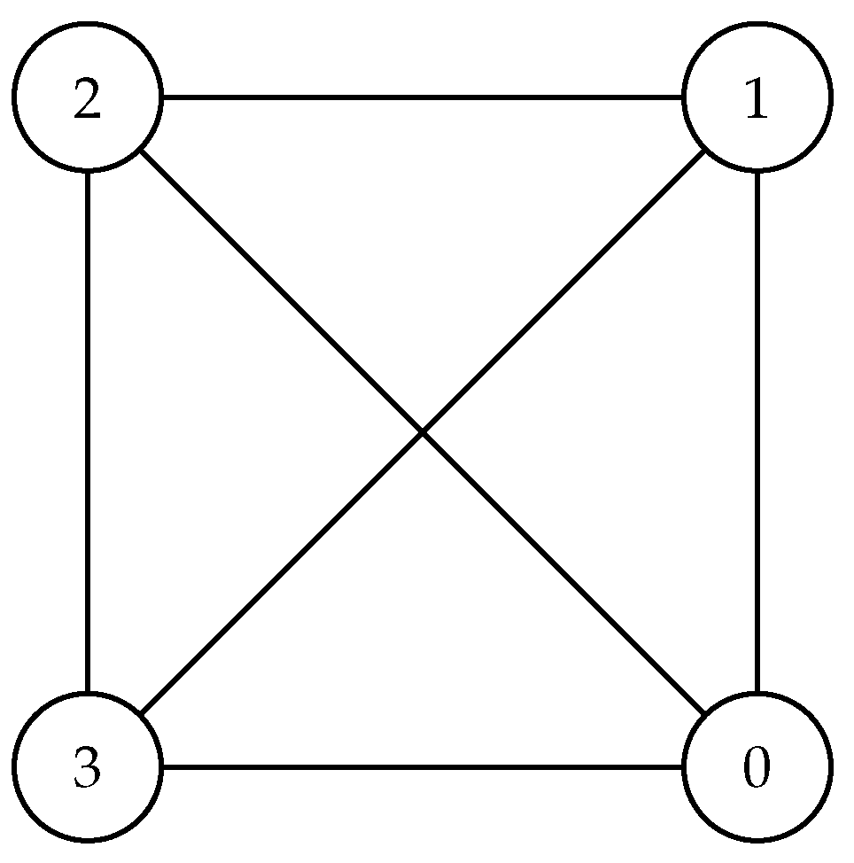
3.1.1. A Four-Node Example

Figure 1 is the graphical depiction of the network $G_1$ consisting of the four nodes $0,1,2$ and 3 together with the arcs that connect them. According to our convention, node 0 is the depot.

Table 2. The input data for the network $G_1$.

Node #	X	Y	Ready Time	Due Date
0	2	2	1	30
1	2	3	14	15
2	3	3	12	25
3	3	4	4	5

gives the quantitative characteristics of the above example: the X and Y coordinates of every node, as well as the Ready Time and the Due Date.

Table 3. The cost matrix for the network $G_1$.

	Node 0	Node 1	Node 2	Node 3
Node 0	0	1	1.41	2.23
Node 1	1	0	1	1.41
Node 2	1.41	1	0	1
Node 3	2.23	1.41	1	0

contains the cost $c_{u,v}$ corresponding to each pair $(u,v)$ of nodes. This cost is taken to reflect the distance between the nodes, which is calculated using the Euclidean distance, given by the well-known formula: $d(u,v)=\sqrt{{(x_2-x_1)}^2+{(y_2-y_1)}^2}$, where $u=(x_1,y_1)$ and $v=(x_2,y_2)$.

A feasible solution for this particular TSPTW is given in

Table 4. A feasible solution for the network $G_1$.

Ordering	Node 0	Node 3	Node 2	Node 1
cost	0 < 1	3.23 < 4	5 < 12	13 < 14
feasibility	yes	yes	yes	yes

. One can see that, if all time windows are respected in every step of a tour going from one customer to the next, a feasible solution can be constructed. Although this is a small scale example, we expect that it will enhance one’s understanding of what is a feasible solution for the TSPTW.

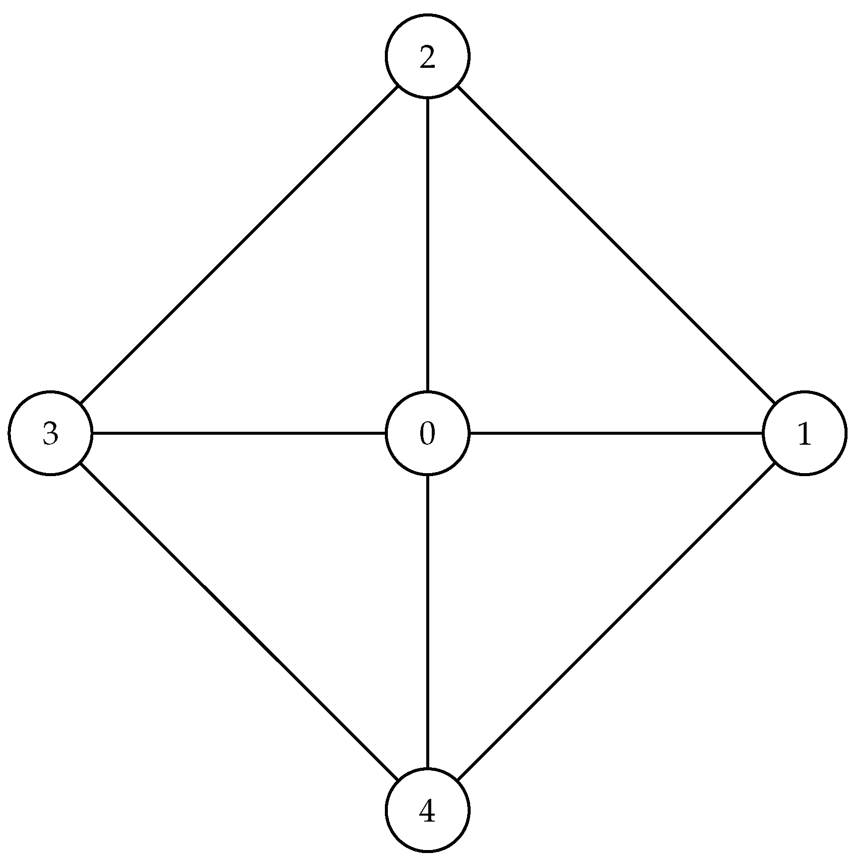
3.1.2. A Five-Node Example

Figure 2 is the pictorial representation depiction of the five-node network $G_2$, where again node 0 is the depot.

Table 5. The input data for the network $G_2$.

Node #	X	Y	Ready Time	Due Date
0	2	2	1	30
1	2	3	14	15
2	3	3	12	25
3	3	4	4	5
4	2	1	8	10

includes all the relevant data for the above example, i.e., the X and Y coordinates of every node, as well as its Ready Time and the Due Date.

Table 6. The cost matrix for the network $G_2$.

	Node 0	Node 1	Node 2	Node 3	Node 4
Node 0	0	1	1.41	2.23	1
Node 1	1	0	1	1.41	2
Node 2	1.41	1	0	1	2.23
Node 3	2.23	1.41	1	0	3.16
Node 4	1	2	2.23	3.16	0

is the cost matrix for the $G_2$ network, where the costs between the nodes again reflect their Euclidean distance.

A feasible solution for this particular TSPTW example is shown in

Table 7. A feasible solution for the network $G_2$.

Ordering	Node 0	Node 3	Node 4	Node 2	Node 1
cost	0 < 1	2.23 < 4	7.16 < 8	10 < 12	12 < 14
feasibility	yes	yes	yes	yes	yes

. One can verify that a feasible tour satisfies the time windows of every customer in each step of the tour.

In the next section, we introduce our novel approach for mapping the TSPTW over the quadratic unconstrained binary optimization (QUBO) model.

4. A QUBO Formulation for the TSPTW

We begin this section by recalling that in the QUBO model we aim to minimize or maximize an expression of the form

$$x^{T}Qx\mathrm{or},\mathrm{in}\mathrm{Dirac}\mathrm{notation},\langle x|Q|x\rangle ,$$

(5)

where x is an n-dimensional column vector of binary decision variables, $x^T$ is the transpose of x, and Q is an $n\times n$ square matrix containing constants.

In the literature, the typical QUBO formulation of the standard TSP involves the use of a set of binary variables (see [33]). They are characterized as binary in the sense that they can take only the 0 or 1 value. Typically, they are denoted by $x_{v,i}$, and their meaning is the following:

$$x_{v,i}=\left\{\begin{array}{cc}\hfill 1,& \mathrm{customer}v\mathrm{is}\mathrm{at}\mathrm{position}i\mathrm{in}\mathrm{the}\mathrm{tour}\hfill \\ \hfill 0,& \mathrm{otherwise}\hfill \end{array}\right..$$

(6)

In the case of the TSPTW, we have discovered it to be more advantageous to use binary variables parameterized by three integers: $u,v$ and i. A similar suggestion for the Vehicle Routing Problem can be found in [39]. Hence, in the rest of our analysis, we use the binary variables $x_{u,v}^i$ defined next

$$x_{u,v}^i=\left\{\begin{array}{cc}\hfill 1,& \mathrm{customers}u\mathrm{and}v\mathrm{are}\mathrm{at}\mathrm{consecutive}\mathrm{positions}i-1\mathrm{and}i\mathrm{in}\mathrm{the}\mathrm{tour}\hfill \\ \hfill 0,& \mathrm{otherwise}\hfill \end{array}\right..$$

(7)

As explained in the previous section, a feasible tour has the form $\{p_0,p_1,\dots ,p_n,p_{n+1}\}$. In this enumeration, $p_i$ is the customer in the ith position of the tour. We always take for granted that $p_0=p_{n+1}=0$ and each other customer appears exactly once. We recall the assumption of zero service time at each customer, and, without loss of generality, we adopt another assumption that greatly reduces the final clutter of our QUBO expressions: for each customer v, where $0\le v\le n$, $e_v=0$. With this understanding, we see that the parameters u and v range from 0 to n and the parameter i ranges from 1 to $n+1$.

Therefore, we can assert that:

• For each i, $1\le i\le n+1$, exactly one of the binary variables $x_{u,v}^i$ is 1, where u and v range freely from 0 to n, with the proviso that $u\ne v$. As a matter of fact, when $i=1$ and $i=n+1$, we can be more precise. In the former case, exactly one of the binary variables $x_{0,v}^1$ is 1, where v ranges from 1 to n, and, in the latter case, exactly one of the binary variables $x_{v,0}^{n+1}$ is 1, where v ranges from 1 to n.
• In addition to the above constraints, for each u, $1\le u\le n$, exactly one of the binary variables $x_{u,v}^i$ is 1, where i ranges from 2 to $n+1$ and v ranges from 1 to n. Obviously, when $i=n+1$, the only relevant decision variable is $x_{u,0}^{n+1}$.
• Symmetrically, we also have the constraint that for every v, $1\le v\le n$, exactly one of the binary variables $x_{u,v}^i$ is 1, where i ranges from 1 to n and u ranges from 1 to n. Again, we point out that, in case $i=1$, the only relevant decision variable is $x_{0,v}^1$.

These constraints are encoded in the Hamiltonian $H_c$.

$$\begin{array}{cc}\hfill H_c=& B{\left(1-\sum _{v=1}^n{x}_{0,v}^1\right)}^2+B\sum _{i=2}^n{\left(1-\sum _{u=1}^n\sum _{\begin{array}{c}v=1\\ v\ne u\end{array}}^n{x}_{u,v}^i\right)}^2+B{\left(1-\sum _{v=1}^n{x}_{v,0}^{n+1}\right)}^2\hfill \\ \hfill +& B\sum _{u=1}^n{\left(1-\left(x_{u,0}^{n+1}+\sum _{i=2}^n\sum _{\begin{array}{c}v=1\\ v\ne u\end{array}}^n{x}_{u,v}^i\right)\right)}^2\hfill \\ \hfill +& B\sum _{v=1}^n{\left(1-\left(x_{0,v}^1+\sum _{i=2}^n\sum _{\begin{array}{c}u=1\\ u\ne v\end{array}}^n{x}_{u,v}^i\right)\right)}^2\hfill \end{array}$$

(8)

Using the $x_{u,v}^i$ binary variables, the requirement that the tour be minimal can be encoded by the following Hamiltonian $H_m$.

$$H_m=C\sum _{i=1}^{n+1}\sum _{u=0}^n\sum _{\begin{array}{c}v=0\\ v\ne u\end{array}}^n{x}_{u,v}^i{c}_{u,v}.$$

(9)

In the above Hamiltonians, B and C are positive constants, which must be appropriately chosen, i.e., $C<B$, so as to ensure that the constraints of $H_c$ are respected (see also [33]). Obviously, $c_{u,v}$ is the cost for traversing the arc $(u,v)$.

Example 1.

To see the form of Equations (8) and (9) in the QUBO framework, we revisit our first example, the network $G_1$.

First, we point out that for binary variables the following holds:

$$\begin{array}{c}\hfill {\left(x_{u,v}^i\right)}^2=x_{u,v}^i.\end{array}$$

(10)

We also recall the identity: ${(a-b-c-d)}^2=a^2+b^2+c^2+d^2-2ab-2ac-2ad+2bc+2bd+2cd$.

The expression ${\left(1-{\sum }_{v=1}^3{x}_{0,v}^1\right)}^2$ in this case can be expanded as

$$\begin{array}{c}\hfill {\left(1-\sum _{v=1}^3{x}_{0,v}^1\right)}^2={(1-x_{0,1}^1-x_{0,2}^1-x_{0,3}^1)}^2\\ \hfill =1+{\left(x_{0,1}^1\right)}^2+{\left(x_{0,2}^1\right)}^2+{\left(x_{0,3}^1\right)}^2-2x_{0,1}^1-2x_{0,2}^1-2x_{0,3}^1+2x_{0,1}^1{x}_{0,2}^1+2x_{0,1}^1{x}_{0,3}^1+2x_{0,2}^1{x}_{0,3}^1\\ \hfill =1+x_{0,1}^1+x_{0,2}^1+x_{0,3}^1-2x_{0,1}^1-2x_{0,2}^1-2x_{0,3}^1+2x_{0,1}^1{x}_{0,2}^1+2x_{0,1}^1{x}_{0,3}^1+2x_{0,2}^1{x}_{0,3}^1\\ \hfill =1-x_{0,1}^1-x_{0,2}^1-x_{0,3}^1+2x_{0,1}^1{x}_{0,2}^1+2x_{0,1}^1{x}_{0,3}^1+2x_{0,2}^1{x}_{0,3}^1\end{array}$$

(*)

In a similar way, we derive the following facts.

$$\begin{array}{c}\hfill \sum _{i=2}^3{\left(1-\sum _{u=1}^3\sum _{\begin{array}{c}v=1\\ v\ne u\end{array}}^3{x}_{u,v}^i\right)}^2\\ \hfill =2-x_{1,2}^2-x_{1,3}^2-x_{2,1}^2-x_{2,3}^2-x_{3,1}^2-x_{3,2}^2-x_{1,2}^3-x_{1,3}^3-x_{2,1}^3-x_{2,3}^3-x_{3,1}^3-x_{3,2}^3\\ \hfill +2x_{1,2}^2{x}_{1,3}^2+2x_{1,2}^2{x}_{2,1}^2+2x_{1,2}^2{x}_{2,3}^2+2x_{1,2}^2{x}_{3,1}^2+2x_{1,2}^2{x}_{3,2}^2+2x_{1,3}^2{x}_{2,1}^2+2x_{1,3}^2{x}_{2,3}^2+2x_{1,3}^2{x}_{3,1}^2+2x_{1,3}^2{x}_{3,2}^2\\ \hfill +2x_{2,1}^2{x}_{2,3}^2+2x_{2,1}^2{x}_{3,1}^2+2x_{2,1}^2{x}_{3,2}^2+2x_{2,3}^2{x}_{3,1}^2+2x_{2,3}^2{x}_{3,2}^2+2x_{3,1}^2{x}_{3,2}^2\\ \hfill +2x_{1,2}^3{x}_{1,3}^3+2x_{1,2}^3{x}_{2,1}^3+2x_{1,2}^3{x}_{2,3}^3+2x_{1,2}^3{x}_{3,1}^3+2x_{1,2}^3{x}_{3,2}^3+2x_{1,3}^3{x}_{2,1}^3+2x_{1,3}^3{x}_{2,3}^3+2x_{1,3}^3{x}_{3,1}^3+2x_{1,3}^3{x}_{3,2}^3\\ \hfill +2x_{2,1}^3{x}_{2,3}^3+2x_{2,1}^3{x}_{3,1}^3+2x_{2,1}^3{x}_{3,2}^3+2x_{2,3}^3{x}_{3,1}^3+2x_{2,3}^3{x}_{3,2}^3+2x_{3,1}^3{x}_{3,2}^3\end{array}$$

(**)

$$\begin{array}{c}\hfill {\left(1-\sum _{v=1}^3{x}_{v,0}^4\right)}^2={(1-x_{1,0}^4-x_{2,0}^4-x_{3,0}^4)}^2=\\ \hfill 1-x_{1,0}^4-x_{2,0}^4-x_{3,0}^4+2x_{1,0}^4{x}_{2,0}^4+2x_{1,0}^4{x}_{3,0}^4+2x_{2,0}^4{x}_{3,0}^4\end{array}$$

(***)

$$\begin{array}{c}\hfill \sum _{u=1}^3{\left(1-\left(x_{u,0}^4+\sum _{i=2}^3\sum _{\begin{array}{c}v=1\\ v\ne u\end{array}}^3{x}_{u,v}^i\right)\right)}^2\\ \hfill =3-x_{1,2}^2-x_{1,3}^2-x_{1,2}^3-x_{1,3}^3-x_{1,0}^4-x_{2,1}^2-x_{2,3}^2-x_{2,1}^3-x_{2,3}^3-x_{2,0}^4-x_{3,1}^2-x_{3,2}^2-x_{3,1}^3-x_{3,2}^3-x_{3,0}^4\\ \hfill +2x_{1,2}^2{x}_{1,3}^2+2x_{1,2}^2{x}_{1,2}^3+2x_{1,2}^2{x}_{1,3}^3+2x_{1,2}^2{x}_{1,0}^4+2x_{1,3}^2{x}_{1,2}^3+2x_{1,3}^2{x}_{1,3}^3+2x_{1,3}^2{x}_{1,0}^4+2x_{1,2}^3{x}_{1,3}^3+2x_{1,2}^3{x}_{1,0}^4+2x_{1,3}^3{x}_{1,0}^4\\ \hfill +2x_{2,1}^2{x}_{2,3}^2+2x_{2,1}^2{x}_{2,1}^3+2x_{2,1}^2{x}_{2,3}^3+2x_{2,1}^2{x}_{2,0}^4+2x_{2,3}^2{x}_{2,1}^3+2x_{2,3}^2{x}_{2,3}^3+2x_{2,3}^2{x}_{2,0}^4+2x_{2,1}^3{x}_{2,3}^3+2x_{2,1}^3{x}_{2,0}^4+2x_{2,3}^3{x}_{1,0}^4\\ \hfill +2x_{3,1}^2{x}_{3,2}^2+2x_{3,1}^2{x}_{3,1}^3+2x_{3,1}^2{x}_{3,2}^3+2x_{3,1}^2{x}_{3,0}^4+2x_{3,2}^2{x}_{3,1}^3+2x_{3,2}^2{x}_{3,2}^3+2x_{3,2}^2{x}_{3,0}^4+2x_{3,1}^3{x}_{3,2}^3+2x_{3,1}^3{x}_{3,0}^4+2x_{3,2}^3{x}_{3,0}^4\end{array}$$

(****)

$$\begin{array}{c}\hfill \sum _{v=1}^3{\left(1-\left(x_{0,v}^1+\sum _{i=2}^3\sum _{\begin{array}{c}u=1\\ u\ne v\end{array}}^3{x}_{u,v}^i\right)\right)}^2\\ \hfill =3-x_{0,1}^1-x_{2,1}^2-x_{3,1}^2-x_{2,1}^3-x_{3,1}^3-x_{0,2}^1-x_{1,2}^2-x_{3,2}^2-x_{1,2}^3-x_{3,2}^3-x_{0,3}^1-x_{1,3}^2-x_{2,3}^2-x_{1,3}^3-x_{2,3}^3\\ \hfill +2x_{0,1}^1{x}_{2,1}^2+2x_{0,1}^1{x}_{3,1}^2+2x_{0,1}^1{x}_{2,1}^3+2x_{0,1}^1{x}_{3,1}^3+2x_{2,1}^2{x}_{3,1}^2+2x_{2,1}^2{x}_{2,1}^3+2x_{2,1}^2{x}_{3,1}^3+2x_{3,1}^2{x}_{2,1}^3+2x_{3,1}^2{x}_{3,1}^3+2x_{2,1}^3{x}_{3,1}^3\\ \hfill +2x_{0,2}^1{x}_{1,2}^2+2x_{0,2}^1{x}_{3,2}^2+2x_{0,2}^1{x}_{1,2}^3+2x_{0,2}^1{x}_{3,2}^3+2x_{1,2}^2{x}_{3,2}^2+2x_{1,2}^2{x}_{1,2}^3+2x_{1,2}^2{x}_{3,2}^3+2x_{3,2}^2{x}_{1,2}^3+2x_{3,2}^2{x}_{3,2}^3+2x_{1,2}^3{x}_{3,2}^3\\ \hfill +2x_{0,3}^1{x}_{1,3}^2+2x_{0,3}^1{x}_{2,3}^2+2x_{0,3}^1{x}_{1,3}^3+2x_{0,3}^1{x}_{2,3}^3+2x_{1,3}^2{x}_{2,3}^2+2x_{1,3}^2{x}_{1,3}^3+2x_{1,3}^2{x}_{2,3}^3+2x_{2,3}^2{x}_{1,3}^3+2x_{2,3}^2{x}_{2,3}^3+2x_{1,3}^3{x}_{2,3}^3\end{array}$$

(*****)

By combining formulas (*)–($*****$), we deduce the Hamiltonian $H_c$ in terms of the binary decision variables.

$$\begin{array}{c}\hfill H_c=10\\ \hfill -2x_{0,1}^1-2x_{0,2}^1-2x_{0,3}^1-3x_{1,2}^2-3x_{1,3}^2-3x_{2,1}^2-3x_{2,3}^2-3x_{3,1}^2-3x_{3,2}^2\\ \hfill -3x_{1,2}^3-3x_{1,3}^3-3x_{2,1}^3-3x_{2,3}^3-3x_{3,1}^3-3x_{3,2}^3-2x_{1,0}^4-2x_{2,0}^4-2x_{3,0}^4\\ \hfill +2x_{0,1}^1{x}_{0,2}^1+2x_{0,1}^1{x}_{0,3}^1+2x_{0,2}^1{x}_{0,3}^1\\ \hfill +2x_{0,1}^1{x}_{2,1}^2+2x_{0,1}^1{x}_{3,1}^2+2x_{0,2}^1{x}_{1,2}^2+2x_{0,2}^1{x}_{3,2}^2+2x_{0,3}^1{x}_{1,3}^2+2x_{0,3}^1{x}_{2,3}^2\\ \hfill +2x_{0,1}^1{x}_{2,1}^3+2x_{0,1}^1{x}_{3,1}^3+2x_{0,2}^1{x}_{1,2}^3+2x_{0,2}^1{x}_{3,2}^3+2x_{0,3}^1{x}_{1,3}^3+2x_{0,3}^1{x}_{2,3}^3\\ \hfill +4x_{1,2}^2{x}_{1,3}^2+2x_{1,2}^2{x}_{2,1}^2+2x_{1,2}^2{x}_{2,3}^2+2x_{1,2}^2{x}_{3,1}^2+4x_{1,2}^2{x}_{3,2}^2+2x_{1,3}^2{x}_{2,1}^2\\ \hfill +4x_{1,3}^2{x}_{2,3}^2+2x_{1,3}^2{x}_{3,1}^2+2x_{1,3}^2{x}_{3,2}^2+4x_{2,1}^2{x}_{2,3}^2+4x_{2,1}^2{x}_{3,1}^2+2x_{2,1}^2{x}_{3,2}^2\\ \hfill +2x_{2,3}^2{x}_{3,1}^2+2x_{2,3}^2{x}_{3,2}^2+4x_{3,1}^2{x}_{3,2}^2\\ \hfill +4x_{1,2}^2{x}_{1,2}^3+2x_{1,2}^2{x}_{1,3}^3+2x_{1,2}^2{x}_{3,2}^3+2x_{1,3}^2{x}_{1,2}^3+4x_{1,3}^2{x}_{1,3}^3+2x_{1,3}^2{x}_{2,3}^3\\ \hfill +4x_{2,1}^2{x}_{2,1}^3+2x_{2,1}^2{x}_{2,3}^3+2x_{2,1}^2{x}_{3,1}^3+2x_{2,3}^2{x}_{1,3}^3+2x_{2,3}^2{x}_{2,1}^3+4x_{2,3}^2{x}_{2,3}^3\\ \hfill +2x_{3,1}^2{x}_{2,1}^3+4x_{3,1}^2{x}_{3,1}^3+2x_{3,1}^2{x}_{3,2}^3+2x_{3,2}^2{x}_{1,2}^3+2x_{3,2}^2{x}_{3,1}^3+4x_{3,2}^2{x}_{3,2}^3\\ \hfill +2x_{1,2}^2{x}_{1,0}^4+2x_{1,3}^2{x}_{1,0}^4+2x_{2,1}^2{x}_{2,0}^4+2x_{2,3}^2{x}_{2,0}^4+2x_{3,1}^2{x}_{3,0}^4+2x_{3,2}^2{x}_{3,0}^4\\ \hfill +4x_{1,2}^3{x}_{1,3}^3+2x_{1,2}^3{x}_{2,1}^3+2x_{1,2}^3{x}_{2,3}^3+2x_{1,2}^3{x}_{3,1}^3+4x_{1,2}^3{x}_{3,2}^3+2x_{1,3}^3{x}_{2,1}^3\\ \hfill +4x_{1,3}^3{x}_{2,3}^3+2x_{1,3}^3{x}_{3,1}^3+2x_{1,3}^3{x}_{3,2}^3+4x_{2,1}^3{x}_{2,3}^3+4x_{2,1}^3{x}_{3,1}^3+2x_{2,1}^3{x}_{3,2}^3\\ \hfill +2x_{2,3}^3{x}_{3,1}^3+2x_{2,3}^3{x}_{3,2}^3+4x_{3,1}^3{x}_{3,2}^3\\ \hfill +2x_{1,2}^3{x}_{1,0}^4+2x_{1,3}^3{x}_{1,0}^4+2x_{2,1}^3{x}_{2,0}^4+2x_{2,3}^3{x}_{1,0}^4+2x_{3,1}^3{x}_{3,0}^4+2x_{3,2}^3{x}_{3,0}^4\\ \hfill +2x_{1,0}^4{x}_{2,0}^4+2x_{1,0}^4{x}_{3,0}^4+2x_{2,0}^4{x}_{3,0}^4\end{array}$$

(11)

Let $X=\left[\begin{array}{c}\hfill x_{0,1}^1\\ \hfill x_{0,2}^1\\ \hfill x_{0,3}^1\\ \hfill x_{1,2}^2\\ \hfill x_{1,3}^2\\ \hfill x_{2,1}^2\\ \hfill x_{2,3}^2\\ \hfill x_{3,1}^2\\ \hfill x_{3,2}^2\\ \hfill x_{1,2}^3\\ \hfill x_{1,3}^3\\ \hfill x_{2,1}^3\\ \hfill x_{2,3}^3\\ \hfill x_{3,1}^3\\ \hfill x_{3,2}^3\\ \hfill x_{1,0}^4\\ \hfill x_{2,0}^4\\ \hfill x_{3,0}^4\end{array}\right]$, $L=\left[\begin{array}{c}\hfill -2\\ \hfill -2\\ \hfill -2\\ \hfill -3\\ \hfill -3\\ \hfill -3\\ \hfill -3\\ \hfill -3\\ \hfill -3\\ \hfill -3\\ \hfill -3\\ \hfill -3\\ \hfill -3\\ \hfill -3\\ \hfill -3\\ \hfill -2\\ \hfill -2\\ \hfill -2\end{array}\right]$, $Q=\left[\begin{array}{cccccccccccccccccc}0& 2& 2& 0& 0& 2& 0& 2& 0& 0& 0& 2& 0& 2& 0& 0& 0& 0\\ 0& 0& 2& 2& 0& 0& 0& 0& 2& 2& 0& 0& 0& 0& 2& 0& 0& 0\\ 0& 0& 0& 0& 2& 0& 2& 0& 0& 0& 2& 0& 2& 0& 0& 0& 0& 0\\ 0& 0& 0& 0& 4& 2& 2& 2& 4& 4& 2& 0& 0& 0& 2& 2& 0& 0\\ 0& 0& 0& 0& 0& 2& 4& 2& 2& 2& 4& 2& 0& 0& 0& 2& 0& 0\\ 0& 0& 0& 0& 0& 0& 4& 4& 2& 0& 0& 4& 2& 2& 0& 0& 2& 0\\ 0& 0& 0& 0& 0& 0& 0& 2& 2& 0& 2& 2& 4& 0& 0& 0& 2& 0\\ 0& 0& 0& 0& 0& 0& 0& 0& 4& 0& 0& 2& 0& 4& 2& 0& 0& 2\\ 0& 0& 0& 0& 0& 0& 0& 0& 0& 2& 0& 0& 0& 2& 4& 0& 0& 2\\ 0& 0& 0& 0& 0& 0& 0& 0& 0& 0& 4& 2& 2& 2& 4& 2& 0& 0\\ 0& 0& 0& 0& 0& 0& 0& 0& 0& 0& 0& 2& 4& 2& 2& 2& 0& 0\\ 0& 0& 0& 0& 0& 0& 0& 0& 0& 0& 0& 0& 4& 4& 2& 0& 2& 0\\ 0& 0& 0& 0& 0& 0& 0& 0& 0& 0& 0& 0& 0& 2& 2& 0& 2& 0\\ 0& 0& 0& 0& 0& 0& 0& 0& 0& 0& 0& 0& 0& 0& 4& 0& 0& 2\\ 0& 0& 0& 0& 0& 0& 0& 0& 0& 0& 0& 0& 0& 0& 0& 0& 0& 2\\ 0& 0& 0& 0& 0& 0& 0& 0& 0& 0& 0& 0& 0& 0& 0& 0& 2& 2\\ 0& 0& 0& 0& 0& 0& 0& 0& 0& 0& 0& 0& 0& 0& 0& 0& 0& 2\\ 0& 0& 0& 0& 0& 0& 0& 0& 0& 0& 0& 0& 0& 0& 0& 0& 0& 0\end{array}\right]$

be the column vector with the binary decision variables, the column vector of the coefficients of the linear terms, and the square matrix of the coefficients of the quadratic terms, respectively. Then, the Hamiltonian $H_c$ can be written more succinctly as $H_c=10+L^{T}X+X^{T}QX$. L and Q contains the qubit biases and the coupling strengths to be used in a future execution of this example on the D-Wave computer.

The above Hamiltonians are certainly not the end of the story in the case of the TSPTW, as, in their essence, they just encode the minimal cost of the Hamiltonian circuit. There are a lot more difficult time constraints to tackle in order to satisfy the time window of every customer. To this end, besides the binary variables $x_{u,v}^i$, it will be necessary to use a second type of binary variables, denoted by $t_{n,i}$, in order to express the time margin of every customer.

Definition 5.

Given a feasible tour $p_0,p_1,\dots ,p_n,p_{n+1}$, suppose that the customer at position i, where $1\le i\le n$, is v with time window $[e_v,l_v]$. We say that the time margin of the customer at position i is $l_v-A_{p_i}$.

Clearly, for a feasible tour, the time margin for every position of the tour is non negative. We can now define the binary variables $t_{k,i}$ as follows:

$$t_{k,i}=\left\{\begin{array}{cc}\hfill 1,& \mathrm{the}\mathrm{time}\mathrm{margin}\mathrm{of}\mathrm{the}\mathrm{customer}\mathrm{at}\mathrm{position}i\mathrm{in}\mathrm{the}\mathrm{tour}\mathrm{is}k\hfill \\ \hfill 0,& \mathrm{otherwise}\hfill \end{array}\right..$$

(12)

We recall that, in the formulation of the TSPTW, the arrival time at the customer in the ith position of the tour, denoted $A_{p_i}$, plays an important role (see [75]). Thus, we begin our analysis by showing how to express $A_{p_i}$. Obviously, $A_{p_0}=0$, thus it is only necessary to give the formula for $A_{p_i}$, $1\le i\le n$. We first observe that the customer at position 0 is always the depot (customer 0), which results in the following, relatively simple, formula, for $A_{p_1}$.

$$A_{p_1}=\sum _{v=1}^n{x}_{0,v}^1{c}_{0,v}.$$

(13)

The general case, i.e., when $2\le i\le n$, is taken care by the next equation.

$$A_{p_i}=\sum _{d=1}^i\sum _{u=1}^n\sum _{\begin{array}{c}v=1\\ v\ne u\end{array}}^n{x}_{u,v}^d{c}_{u,v}(2\le i\le n).$$

(14)

Example 2.

To explain how Equations (13) and (14) can be used in practice, we examine the network $G_2$.

Equation (13) becomes

$$A_{p_1}=x_{0,1}^1{c}_{0,1}+x_{0,2}^1{c}_{0,2}+x_{0,3}^1{c}_{0,3}+x_{0,4}^1{c}_{0,4}$$

(15)

Equation (14) gives the following series of equations.

$$\begin{array}{cc}\hfill A_{p_2}=& \left(\underset{A_{p_1}}{\underbrace{x_{0,1}^1{c}_{0,1}+x_{0,2}^1{c}_{0,2}+x_{0,3}^1{c}_{0,3}+x_{0,4}^1{c}_{0,4}}}\right)\hfill \\ \hfill +& x_{1,2}^2{c}_{1,2}+x_{1,3}^2{c}_{1,3}+x_{1,4}^2{c}_{1,4}+x_{2,1}^2{c}_{2,1}+x_{2,3}^2{c}_{2,3}+x_{2,4}^2{c}_{2,4}\hfill \\ \hfill +& x_{3,1}^2{c}_{3,1}+x_{3,2}^2{c}_{3,2}+x_{3,4}^2{c}_{3,4}+x_{4,1}^2{c}_{4,1}+x_{4,2}^2{c}_{4,2}+x_{4,3}^2{c}_{4,3}\hfill \end{array}$$

(16)

$$\begin{array}{cc}\hfill A_{p_3}=& (\left(x_{0,1}^1{c}_{0,1}+x_{0,2}^1{c}_{0,2}+x_{0,3}^1{c}_{0,3}+x_{0,4}^1{c}_{0,4}\right)\hfill \\ \hfill +& x_{1,2}^2{c}_{1,2}+x_{1,3}^2{c}_{1,3}+x_{1,4}^2{c}_{1,4}+x_{2,1}^2{c}_{2,1}+x_{2,3}^2{c}_{2,3}+x_{2,4}^2{c}_{2,4}\hfill \\ \hfill +& x_{3,1}^2{c}_{3,1}+x_{3,2}^2{c}_{3,2}+x_{3,4}^2{c}_{3,4}+x_{4,1}^2{c}_{4,1}+x_{4,2}^2{c}_{4,2}+x_{4,3}^2{c}_{4,3})\hfill \\ \hfill +& x_{1,2}^3{c}_{1,2}+x_{1,3}^3{c}_{1,3}+x_{1,4}^3{c}_{1,4}+x_{2,1}^3{c}_{2,1}+x_{2,3}^3{c}_{2,3}+x_{2,4}^3{c}_{2,4}\hfill \\ \hfill +& x_{3,1}^3{c}_{3,1}+x_{3,2}^3{c}_{3,2}+x_{3,4}^3{c}_{3,4}+x_{4,1}^3{c}_{4,1}+x_{4,2}^3{c}_{4,2}+x_{4,3}^3{c}_{4,3}\hfill \end{array}$$

(17)

$$\begin{array}{cc}\hfill A_{p_4}=& x_{0,1}^1{c}_{0,1}+x_{0,2}^1{c}_{0,2}+x_{0,3}^1{c}_{0,3}+x_{0,4}^1{c}_{0,4}\hfill \\ \hfill +& x_{1,2}^2{c}_{1,2}+x_{1,3}^2{c}_{1,3}+x_{1,4}^2{c}_{1,4}+x_{2,1}^2{c}_{2,1}+x_{2,3}^2{c}_{2,3}+x_{2,4}^2{c}_{2,4}\hfill \\ \hfill +& x_{3,1}^2{c}_{3,1}+x_{3,2}^2{c}_{3,2}+x_{3,4}^2{c}_{3,4}+x_{4,1}^2{c}_{4,1}+x_{4,2}^2{c}_{4,2}+x_{4,3}^2{c}_{4,3}\hfill \\ \hfill +& x_{1,2}^3{c}_{1,2}+x_{1,3}^3{c}_{1,3}+x_{1,4}^3{c}_{1,4}+x_{2,1}^3{c}_{2,1}+x_{2,3}^3{c}_{2,3}+x_{2,4}^3{c}_{2,4}\hfill \\ \hfill +& x_{3,1}^3{c}_{3,1}+x_{3,2}^3{c}_{3,2}+x_{3,4}^3{c}_{3,4}+x_{4,1}^3{c}_{4,1}+x_{4,2}^3{c}_{4,2}+x_{4,3}^3{c}_{4,3}\hfill \\ \hfill +& x_{1,2}^4{c}_{1,2}+x_{1,3}^4{c}_{1,3}+x_{1,4}^4{c}_{1,4}+x_{2,1}^4{c}_{2,1}+x_{2,3}^4{c}_{2,3}+x_{2,4}^4{c}_{2,4}\hfill \\ \hfill +& x_{3,1}^4{c}_{3,1}+x_{3,2}^4{c}_{3,2}+x_{3,4}^4{c}_{3,4}+x_{4,1}^4{c}_{4,1}+x_{4,2}^4{c}_{4,2}+x_{4,3}^4{c}_{4,3}\hfill \end{array}$$

(18)

The above equations demonstrate that, in every case, $A_{p_i}$ can be expressed as a sum of terms, where each term is the product of an input variable $c_{u,v}$ and exactly one binary decision variable $x_{u,v}^i$.

The simplifying assumption of zero service time enables us to express the constraints imposed by the time windows of every customer as follows:

$$A_{p_1}\le \sum _{v=1}^n{x}_{0,v}^1{l}_v,$$

(19)

for the special case where $i=1$, and

$$A_{p_i}\le \sum _{u=1}^n\sum _{\begin{array}{c}v=1\\ v\ne u\end{array}}^n{x}_{u,v}^i{l}_v(2\le i\le n),$$

(20)

for the general case where $2\le i\le n$.

The above expression may seem a little complicated, but, unfortunately, while $A_{p_i}$ tells us the arrival time at the customer in the ith position of the tour, it does not tell us which is this particular customer. We have to resort to the binary variables $x_{u,v}^i$ to indirectly obtain this information.

Inequality constraints such as these in Equations (19) and (20) are notoriously difficult to express within the QUBO framework. For an extensive analysis, we refer the interested reader to [29,64,76]. The approach which is most commonly used in the literature is to employ auxiliary binary variables, such as the binary variables $t_{k,i}$ previously defined, to convert the inequality into an equality, and then proceed, as usual, by squaring the equality constraint.

In our case, the first step is to express the inequalities in Equations (19) and (20) as

$$A_{p_1}+\sum _{k=1}^{K}k{t}_{k,1}=\sum _{v=1}^n{x}_{0,v}^1{l}_v,$$

(21)

and

$$A_{p_i}+\sum _{k=1}^{K}k{t}_{k,i}=\sum _{u=1}^n\sum _{\begin{array}{c}v=1\\ v\ne u\end{array}}^n{x}_{u,v}^i{l}_v(2\le i\le n),$$

(22)

respectively.

In the above equalities, K is a positive constant appropriately chosen taking into consideration the specific time windows. A valid possible choice could be $K={max}_{1\le v\le n}\left\{l_v\right\}$. Such a choice, while valid, would be unnecessarily big in most practical cases.

Equality constraints such as Equations (21) and (22) are typically treated in QUBO by converting them into squared expressions. Hence, Equation (21) gives rise to the first time window constraint, denoted by $W_1$ and given by

$$\begin{array}{c}\hfill W_1={\left(A_{p_1}+\sum _{k=1}^{K}k{t}_{k,i}-\sum _{v=1}^n{x}_{0,v}^1{l}_v\right)}^2,\end{array}$$

(23)

while Equation (22) gives rise to the ith time window constraint, denoted by $W_i$ and given by

$$\begin{array}{c}\hfill W_i={\left(A_{p_i}+\sum _{k=1}^{K}k{t}_{k,i}-\sum _{u=1}^n\sum _{\begin{array}{c}v=1\\ v\ne u\end{array}}^n{x}_{u,v}^i{l}_v\right)}^2(2\le i\le n).\end{array}$$

(24)

If we replace $A_{p_1}$ and $A_{p_i}$ in the above equations by Equations (13) and (14), we derive the expanded forms of $W_1$ and $W_i$, $2\le i\le n$, respectively.

$$\begin{array}{c}\hfill W_1={\left(\sum _{v=1}^n{x}_{0,v}^1{c}_{0,v}+\sum _{k=1}^{K}k{t}_{k,i}-\sum _{v=1}^n{x}_{0,v}^1{l}_v\right)}^2.\end{array}$$

(25)

$$\begin{array}{c}\hfill W_i={\left(\sum _{d=1}^i\sum _{u=1}^n\sum _{\begin{array}{c}v=1\\ v\ne u\end{array}}^n{x}_{u,v}^d{c}_{u,v}+\sum _{k=1}^{K}k{t}_{k,i}-\sum _{u=1}^n\sum _{\begin{array}{c}v=1\\ v\ne u\end{array}}^n{x}_{u,v}^i{l}_v\right)}^2(2\le i\le n).\end{array}$$

(26)

At this point, it is important to pause and confirm that the constraints in Equations (25) and (26) conform to the QUBO formulation requirements, in the sense that, after the expansion of the square, we get a sum of terms, where each term is the product of input data such as $c_{u,v}$ or $l_v$ and at most two binary decision variables.

The last time constraint concerns the binary variables $t_{k,i}$. For each i, $1\le i\le n$, exactly one of the binary variables $t_{k,i}$ is 1, where k ranges from 1 to K. The meaning of this constraint is obvious: in every position of a feasible tour the time margin should be unique. Expressing this constraint is also straightforward:

$$M_i={\left(1-\sum _{k=1}^K{t}_{k,i}\right)}^2(1\le i\le n).$$

(27)

Putting all the time constraints together results in the Hamiltonian $H_t$:

$$\begin{array}{c}\hfill H_t=T\left(W_1\right)+T\sum _{i=2}^{n}TW{C}_i+T\sum _{i=1}^n{M}_i.\end{array}$$

(28)

Therefore, to solve the TSPTW in the QUBO framework we must use the Hamiltonian H given below:

$$\begin{array}{c}\hfill H=H_c+H_m+H_t.\end{array}$$

(29)

As noted above, the constants B, C and T appearing in the Hamiltonians are positive constants, which must be chosen according to our requirements. For instance, by setting $C<B$, so as to ensure that the constraints of $H_c$ are respected; similarly, setting $T<B$ prioritizes the time windows constraints over the minimality of the tour.

Example 3.

To show the form of the time windows constraints when the square is expanded, we apply the constraint in Equation (25) to network $G_2$.

We point out that for binary variables the following hold:

$$\begin{array}{c}\hfill {\left(x_{u,v}^i\right)}^2=x_{u,v}^{i}and{\left(t_{k,i}\right)}^2=t_{k,i}.\end{array}$$

(30)

We also recall the identity: ${(a+b-c)}^2=a^2+b^2+c^2+2ab-2ac-2bc$. We use this identity to expand Equation (25), setting $a={\sum }_{v=1}^n{x}_{0,v}^1{c}_{0,v}$, $b={\sum }_{k=1}^{K}k{t}_{k,1}$, and $c={\sum }_{v=1}^n{x}_{0,v}^1{l}_v$. In our example, $n=4$ and, to simplify somewhat the calculations, we take $K=2$. With this understanding, we use Equation (15) to derive the formulas given below. Note that to improve the readability of the equations in this example, we have written in green color those terms that involve exactly one binary variable and in blue color those terms that involve exactly two binary variables.

$$\begin{array}{cc}\hfill A_{p_1}^2=& {\left(x_{0,1}^1{c}_{0,1}+x_{0,2}^1{c}_{0,2}+x_{0,3}^1{c}_{0,3}+x_{0,4}^1{c}_{0,4}\right)}^2\hfill \\ \hfill =& {\left(x_{0,1}^1\right)}^2{c}_{0,1}^2+{\left(x_{0,2}^1\right)}^2{c}_{0,2}^2+{\left(x_{0,3}^1\right)}^2{c}_{0,3}^2+{\left(x_{0,4}^1\right)}^2{c}_{0,4}^2+2x_{0,1}^1{c}_{0,1}{x}_{0,2}^1{c}_{0,2}+2x_{0,1}^1{c}_{0,1}{x}_{0,3}^1{c}_{0,3}\hfill \\ \hfill +& 2x_{0,1}^1{c}_{0,1}{x}_{0,4}^1{c}_{0,4}+2x_{0,2}^1{c}_{0,2}{x}_{0,3}^1{c}_{0,3}+2x_{0,2}^1{c}_{0,2}{x}_{0,4}^1{c}_{0,4}+2x_{0,3}^1{c}_{0,3}{x}_{0,4}^1{c}_{0,4}\hfill \\ \hfill =& x_{0,1}^1{c}_{0,1}^2+x_{0,2}^1{c}_{0,2}^2+x_{0,3}^1{c}_{0,3}^2+x_{0,4}^1{c}_{0,4}^2+2x_{0,1}^1{c}_{0,1}{x}_{0,2}^1{c}_{0,2}+2x_{0,1}^1{c}_{0,1}{x}_{0,3}^1{c}_{0,3}\hfill \\ \hfill +& 2x_{0,1}^1{c}_{0,1}{x}_{0,4}^1{c}_{0,4}+2x_{0,2}^1{c}_{0,2}{x}_{0,3}^1{c}_{0,3}+2x_{0,2}^1{c}_{0,2}{x}_{0,4}^1{c}_{0,4}+2x_{0,3}^1{c}_{0,3}{x}_{0,4}^1{c}_{0,4}\hfill \end{array}$$

(31)

Similarly, we see that:

$$\begin{array}{c}\hfill {\left(\sum _{k=1}^{2}k{t}_{k,1}\right)}^2={\left(1t_{1,1}+2t_{2,1}\right)}^2=t_{1,1}^2+4t_{2,1}^2+4t_{1,1}{t}_{2,1}=t_{1,1}+4t_{2,1}+4t_{1,1}{t}_{2,1}\end{array}$$

(32)

$$\begin{array}{cc}\hfill {\left(\sum _{v=1}^4{x}_{0,v}^1{l}_v\right)}^2=& {\left(x_{0,1}^1{l}_1+x_{0,2}^1{l}_2+x_{0,3}^1{l}_3+x_{0,4}^1{l}_4\right)}^2\hfill \\ \hfill =& {\left(x_{0,1}^1\right)}^2{l}_1^2+{\left(x_{0,2}^1\right)}^2{l}_2^2+{\left(x_{0,3}^1\right)}^2{l}_3^2+{\left(x_{0,4}^1\right)}^2{l}_4^2+2x_{0,1}^1{l}_1{x}_{0,2}^1{l}_2+2x_{0,1}^1{l}_1{x}_{0,3}^1{l}_3\hfill \\ \hfill +& 2x_{0,1}^1{l}_1{x}_{0,4}^1{l}_4+2x_{0,2}^1{l}_2{x}_{0,3}^1{l}_3+2x_{0,2}^1{l}_2{x}_{0,4}^1{l}_4+2x_{0,3}^1{l}_3{x}_{0,4}^1{l}_4\hfill \\ \hfill =& x_{0,1}^1{l}_1^2+x_{0,2}^1{l}_2^2+x_{0,3}^1{l}_3^2+x_{0,4}^1{l}_4^2+2x_{0,1}^1{l}_1{x}_{0,2}^1{l}_2+2x_{0,1}^1{l}_1{x}_{0,3}^1{l}_3\hfill \\ \hfill +& 2x_{0,1}^1{l}_1{x}_{0,4}^1{l}_4+2x_{0,2}^1{l}_2{x}_{0,3}^1{l}_3+2x_{0,2}^1{l}_2{x}_{0,4}^1{l}_4+2x_{0,3}^1{l}_3{x}_{0,4}^1{l}_4\hfill \end{array}$$

(33)

$$\begin{array}{cc}\hfill 2A_{p_1}\sum _{k=1}^{2}k{t}_{k,1}=& 2\left(x_{0,1}^1{c}_{0,1}+x_{0,2}^1{c}_{0,2}+x_{0,3}^1{c}_{0,3}+x_{0,4}^1{c}_{0,4}\right)\left(1t_{1,1}+2t_{2,1}\right)\hfill \\ \hfill =& 2x_{0,1}^1{c}_{0,1}{t}_{1,1}+2x_{0,1}^1{c}_{0,1}{t}_{2,1}+2x_{0,2}^1{c}_{0,2}{t}_{1,1}+2x_{0,2}^1{c}_{0,2}{t}_{2,1}\hfill \\ \hfill +& 2x_{0,3}^1{c}_{0,3}{t}_{1,1}+2x_{0,3}^1{c}_{0,3}{t}_{2,1}+2x_{0,4}^1{c}_{0,4}{t}_{1,1}+2x_{0,4}^1{c}_{0,4}{t}_{2,1}\hfill \end{array}$$

(34)

$$\begin{array}{cc}\hfill 2A_{p_1}\sum _{v=1}^4{x}_{0,v}^1{l}_v=& 2\left(x_{0,1}^1{c}_{0,1}+x_{0,2}^1{c}_{0,2}+x_{0,3}^1{c}_{0,3}+x_{0,4}^1{c}_{0,4}\right)\left(x_{0,1}^1{l}_1+x_{0,2}^1{l}_2+x_{0,3}^1{l}_3+x_{0,4}^1{l}_4\right)\hfill \\ \hfill =& 2{\left(x_{0,1}^1\right)}^2{c}_{0,1}{l}_1+2x_{0,1}^1{c}_{0,1}{x}_{0,2}^1{l}_2+2x_{0,1}^1{c}_{0,1}{x}_{0,3}^1{l}_3+2x_{0,1}^1{c}_{0,1}{x}_{0,4}^1{l}_4\hfill \\ \hfill +& 2x_{0,2}^1{c}_{0,2}{x}_{0,1}^1{l}_1+2{\left(x_{0,2}^1\right)}^2{c}_{0,2}{l}_2+2x_{0,2}^1{c}_{0,2}{x}_{0,3}^1{l}_3+2x_{0,2}^1{c}_{0,2}{x}_{0,4}^1{l}_4\hfill \\ \hfill +& 2x_{0,3}^1{c}_{0,3}{x}_{0,1}^1{l}_1+2x_{0,3}^1{c}_{0,3}{x}_{0,2}^1{l}_2+2{\left(x_{0,3}^1\right)}^2{c}_{0,3}{l}_3+2x_{0,3}^1{c}_{0,3}{x}_{0,4}^1{l}_4\hfill \\ \hfill +& 2x_{0,4}^1{c}_{0,4}{x}_{0,1}^1{l}_1+2x_{0,4}^1{c}_{0,4}{x}_{0,2}^1{l}_2+2x_{0,4}^1{c}_{0,4}{x}_{0,3}^1{l}_3+2{\left(x_{0,4}^1\right)}^2{c}_{0,4}{l}_4\hfill \\ \hfill =& 2x_{0,1}^1{c}_{0,1}{l}_1+2x_{0,2}^1{c}_{0,2}{l}_2+2x_{0,3}^1{c}_{0,3}{l}_3+2x_{0,4}^1{c}_{0,4}{l}_4\hfill \\ \hfill +& 2x_{0,1}^1{c}_{0,1}{x}_{0,2}^1{l}_2+2x_{0,1}^1{c}_{0,1}{x}_{0,3}^1{l}_3+2x_{0,1}^1{c}_{0,1}{x}_{0,4}^1{l}_4\hfill \\ \hfill +& 2x_{0,2}^1{c}_{0,2}{x}_{0,1}^1{l}_1+2x_{0,2}^1{c}_{0,2}{x}_{0,3}^1{l}_3+2x_{0,2}^1{c}_{0,2}{x}_{0,4}^1{l}_4\hfill \\ \hfill +& 2x_{0,3}^1{c}_{0,3}{x}_{0,1}^1{l}_1+2x_{0,3}^1{c}_{0,3}{x}_{0,2}^1{l}_2+2x_{0,3}^1{c}_{0,3}{x}_{0,4}^1{l}_4\hfill \\ \hfill +& 2x_{0,4}^1{c}_{0,4}{x}_{0,1}^1{l}_1+2x_{0,4}^1{c}_{0,4}{x}_{0,2}^1{l}_2+2x_{0,4}^1{c}_{0,4}{x}_{0,3}^1{l}_3\hfill \end{array}$$

(35)

$$\begin{array}{cc}\hfill 2\sum _{k=1}^{2}k{t}_{k,1}\sum _{v=1}^4{x}_{0,v}^1{l}_v=& 2\left(1t_{1,1}+2t_{2,1}\right)\left(x_{0,1}^1{l}_1+x_{0,2}^1{l}_2+x_{0,3}^1{l}_3+x_{0,4}^1{l}_4\right)\hfill \\ \hfill =& 2t_{1,1}{x}_{0,1}^1{l}_1+2t_{1,1}{x}_{0,2}^1{l}_2+2t_{1,1}{x}_{0,3}^1{l}_3+2t_{1,1}{x}_{0,4}^1{l}_4\hfill \\ \hfill +& 4t_{2,1}{x}_{0,1}^1{l}_1+4t_{2,1}{x}_{0,2}^1{l}_2+4t_{2,1}{x}_{0,3}^1{l}_3+4t_{2,1}{x}_{0,4}^1{l}_4\hfill \end{array}$$

(36)

We can now substitute Equations (31)–(36) into Equation (25) to finally arrive at the expanded form of the constraint, given by the following equation.

$$\begin{array}{cc}\hfill W_1=& x_{0,1}^1{c}_{0,1}^2+x_{0,2}^1{c}_{0,2}^2+x_{0,3}^1{c}_{0,3}^2+x_{0,4}^1{c}_{0,4}^2+2x_{0,1}^1{c}_{0,1}{x}_{0,2}^1{c}_{0,2}+2x_{0,1}^1{c}_{0,1}{x}_{0,3}^1{c}_{0,3}\hfill \\ \hfill +& 2x_{0,1}^1{c}_{0,1}{x}_{0,4}^1{c}_{0,4}+2x_{0,2}^1{c}_{0,2}{x}_{0,3}^1{c}_{0,3}+2x_{0,2}^1{c}_{0,2}{x}_{0,4}^1{c}_{0,4}+2x_{0,3}^1{c}_{0,3}{x}_{0,4}^1{c}_{0,4}\hfill \\ \hfill +& t_{1,1}+4t_{2,1}+4t_{1,1}{t}_{2,1}\hfill \\ \hfill +& x_{0,1}^1{l}_1^2+x_{0,2}^1{l}_2^2+x_{0,3}^1{l}_3^2+x_{0,4}^1{l}_4^2+2x_{0,1}^1{l}_1{x}_{0,2}^1{l}_2+2x_{0,1}^1{l}_1{x}_{0,3}^1{l}_3\hfill \\ \hfill +& 2x_{0,1}^1{l}_1{x}_{0,4}^1{l}_4+2x_{0,2}^1{l}_2{x}_{0,3}^1{l}_3+2x_{0,2}^1{l}_2{x}_{0,4}^1{l}_4+2x_{0,3}^1{l}_3{x}_{0,4}^1{l}_4\hfill \\ \hfill -& 2x_{0,1}^1{c}_{0,1}{t}_{1,1}-2x_{0,1}^1{c}_{0,1}{t}_{2,1}-2x_{0,2}^1{c}_{0,2}{t}_{1,1}-2x_{0,2}^1{c}_{0,2}{t}_{2,1}\hfill \\ \hfill -& 2x_{0,3}^1{c}_{0,3}{t}_{1,1}-2x_{0,3}^1{c}_{0,3}{t}_{2,1}-2x_{0,4}^1{c}_{0,4}{t}_{1,1}-2x_{0,4}^1{c}_{0,4}{t}_{2,1}\hfill \\ \hfill -& 2x_{0,1}^1{c}_{0,1}{l}_1-2x_{0,2}^1{c}_{0,2}{l}_2-2x_{0,3}^1{c}_{0,3}{l}_3-2x_{0,4}^1{c}_{0,4}{l}_4\hfill \\ \hfill -& 2x_{0,1}^1{c}_{0,1}{x}_{0,2}^1{l}_2-2x_{0,1}^1{c}_{0,1}{x}_{0,3}^1{l}_3-2x_{0,1}^1{c}_{0,1}{x}_{0,4}^1{l}_4\hfill \\ \hfill -& 2x_{0,2}^1{c}_{0,2}{x}_{0,1}^1{l}_1-2x_{0,2}^1{c}_{0,2}{x}_{0,3}^1{l}_3-2x_{0,2}^1{c}_{0,2}{x}_{0,4}^1{l}_4\hfill \\ \hfill -& 2x_{0,3}^1{c}_{0,3}{x}_{0,1}^1{l}_1-2x_{0,3}^1{c}_{0,3}{x}_{0,2}^1{l}_2-2x_{0,3}^1{c}_{0,3}{x}_{0,4}^1{l}_4\hfill \\ \hfill -& 2x_{0,4}^1{c}_{0,4}{x}_{0,1}^1{l}_1-2x_{0,4}^1{c}_{0,4}{x}_{0,2}^1{l}_2-2x_{0,4}^1{c}_{0,4}{x}_{0,3}^1{l}_3\hfill \\ \hfill -& 2t_{1,1}{x}_{0,1}^1{l}_1-2t_{1,1}{x}_{0,2}^1{l}_2-2t_{1,1}{x}_{0,3}^1{l}_3-2t_{1,1}{x}_{0,4}^1{l}_4\hfill \\ \hfill -& 4t_{2,1}{x}_{0,1}^1{l}_1-4t_{2,1}{x}_{0,2}^1{l}_2-4t_{2,1}{x}_{0,3}^1{l}_3-4t_{2,1}{x}_{0,4}^1{l}_4\hfill \end{array}$$

(37)

Similar calculations, albeit too lengthy to include here, confirm that all time window constraints have similar patterns, that is they constitute legitimate expressions within the QUBO framework.

5. Conclusions and Future Work

In this work, we consider the TSPTW. Although many combinatorial optimization problems have been expressed in the QUBO (or, equivalently, the Ising) formulation, this particular problem was not one of them. Presumably, the reason is the TSPTW imposes many additional (time) constraints because the customers’ time windows must be satisfied. These are actually inequality constraints that are very difficult to tackle within the QUBO framework. We remind the reader that valid QUBO expressions must have the form: $x^{T}Qx$, where x is a column vector of binary decision variables, $x^T$ its transpose and Q a square matrix of constants. Thus, to the best of our knowledge, this is the first time the TSPTW is cast in QUBO form.

This step is a necessary precondition order to be able to run TSPTW instances on the current generation of D-Wave computers. Hence, the future direction of this work will the mapping of TSPTW benchmarks to the Chimera or the upcoming Pegasus architecture, so as to obtain experimental results. This will enable the comparison of the current state-of-the-art classical, or conventional, if you prefer, metaheuristics with the purely quantum approach. This comparison is expected to shed some light on the pressing question of whether quantum annealing is more efficient than classical methods, and, if so, to what degree.

References

Feynman, R.P. Simulating physics with computers. Int. J. Theor. Phys.1982, 21, 467–488. [Google Scholar] [CrossRef]
Shor, P.W. Polynomial-time algorithms for prime factorization and discrete logarithms on a quantum computer. SIAM Rev.1999, 41, 303–332. [Google Scholar] [CrossRef]
Grover, L. A fast quantum mechanical algorithm for database search. In Proceedings of the Twenty-Eighth Annual ACM Symposium on the Theory of Computing, Philadelphia, PA, USA, 22–24 May 1996. [Google Scholar]
Nielsen, M.A.; Chuang, I.L. Quantum Computation and Quantum Information; Cambridge University Press: Cambridge, UK, 2010. [Google Scholar]
Farhi, E.; Goldstone, J.; Gutmann, S.; Sipser, M. Quantum computation by adiabatic evolution. arXiv2000, arXiv:quant-ph/0001106. [Google Scholar]
Farhi, E.; Goldstone, J.; Gutmann, S.; Lapan, J.; Lundgren, A.; Preda, D. A quantum adiabatic evolution algorithm applied to random instances of an NP-complete problem. Science2001, 292, 472–475. [Google Scholar] [CrossRef]
Choi, V. Minor-embedding in adiabatic quantum computation: I. The parameter setting problem. Quantum Inf. Process.2008, 7, 193–209. [Google Scholar] [CrossRef]
Messiah, A. Quantum Mechanics; Dover Publications: New York, NY, USA, 1961. [Google Scholar]
Amin, M. Consistency of the adiabatic theorem. Phys. Rev. Lett.2009, 102, 220401. [Google Scholar] [CrossRef]
Aharonov, D.; van Dam, W.; Kempe, J.; Landau, Z.; Lloyd, S.; Regev, O. Adiabatic Quantum Computation Is Equivalent to Standard Quantum Computation. SIAM Rev.2008, 50, 755–787. [Google Scholar] [CrossRef]
Kadowaki, T. Study of optimization problems by quantum annealing. arXiv2002, arXiv:quant-ph/0205020. [Google Scholar]
Kadowaki, T.; Nishimori, H. Quantum annealing in the transverse Ising model. Phys. Rev. E1998, 58, 5355. [Google Scholar] [CrossRef]
Pakin, S. Performing fully parallel constraint logic programming on a quantum annealer. Theory Pract. Logic Programm.2018, 18, 928–949. [Google Scholar] [CrossRef]
Perdomo-Ortiz, A.; Dickson, N.; Drew-Brook, M.; Rose, G.; Aspuru-Guzik, A. Finding low-energy conformations of lattice protein models by quantum annealing. Sci. Rep.2012, 2, 571. [Google Scholar] [CrossRef] [PubMed]
Sarkar, A. Quantum Algorithms: For Pattern-Matching in Genomic Sequences. Master’s Thesis, Delft University of Technology, Delft, The Netherlands, 2018. [Google Scholar]
Rebentrost, P.; Schuld, M.; Wossnig, L.; Petruccione, F.; Lloyd, S. Quantum gradient descent and Newton’s method for constrained polynomial optimization. New J. Phys.2019, 21, 073023. [Google Scholar] [CrossRef]
Dattani, N.; Szalay, S.; Chancellor, N. Pegasus: The second connectivity graph for large-scale quantum annealing hardware. arXiv2019, arXiv:1901.07636. [Google Scholar]
Dattani, N.; Chancellor, N. Embedding quadratization gadgets on Chimera and Pegasus graphs. arXiv2019, arXiv:1901.07676. [Google Scholar]
Lewis, M.; Glover, F. Quadratic unconstrained binary optimization problem preprocessing: Theory and empirical analysis. Networks2017, 70, 79–97. [Google Scholar] [CrossRef]
Kochenberger, G.; Hao, J.K.; Glover, F.; Lewis, M.; Lü, Z.; Wang, H.; Wang, Y. The unconstrained binary quadratic programming problem: A survey. J. Comb. Optim.2014, 28, 58–81. [Google Scholar] [CrossRef]
Lloyd, S.; Mohseni, M.; Rebentrost, P. Quantum algorithms for supervised and unsupervised machine learning. arXiv2013, arXiv:1307.0411. [Google Scholar]
Glover, F.; Kochenberger, G. A Tutorial on Formulating QUBO Models. arXiv2018, arXiv:1811.11538. [Google Scholar]
Boros, E.; Hammer, P.L.; Tavares, G. Local search heuristics for quadratic unconstrained binary optimization (QUBO). J. Heuristics2007, 13, 99–132. [Google Scholar] [CrossRef]
Ushijima-Mwesigwa, H.; Negre, C.F.; Mniszewski, S.M. Graph partitioning using quantum annealing on the D-Wave system. In Proceedings of the Second International Workshop on Post Moores Era Supercomputing, Denver, CO, USA, 12–17 November 2017; ACM: New York, NY, USA, 2017; pp. 22–29. [Google Scholar]
Newell, G.F.; Montroll, E.W. On the theory of the Ising model of ferromagnetism. Rev. Mod. Phys.1953, 25, 353. [Google Scholar] [CrossRef]
Lucas, A. Ising formulations of many NP problems. Front. Phys.2014, 2, 5. [Google Scholar] [CrossRef]
Neukart, F.; Compostella, G.; Seidel, C.; Von Dollen, D.; Yarkoni, S.; Parney, B. Traffic flow optimization using a quantum annealer. Front. ICT2017, 4, 29. [Google Scholar] [CrossRef]
Martoňák, R.; Santoro, G.E.; Tosatti, E. Quantum annealing of the traveling-salesman problem. Phys. Rev. E2004, 70, 057701. [Google Scholar] [CrossRef]
Warren, R.H. Adapting the traveling salesman problem to an adiabatic quantum computer. Quantum Inf. Process.2013, 12, 1781–1785. [Google Scholar] [CrossRef]
Warren, R.H. Small traveling salesman problems. J. Adv. Appl. Math.2017, 2. [Google Scholar] [CrossRef]
Feld, S.; Roch, C.; Gabor, T.; Seidel, C.; Neukart, F.; Galter, I.; Mauerer, W.; Linnhoff-Popien, C. A hybrid solution method for the capacitated vehicle routing problem using a quantum annealer. arXiv2018, arXiv:1811.07403. [Google Scholar] [CrossRef]
Irie, H.; Wongpaisarnsin, G.; Terabe, M.; Miki, A.; Taguchi, S. Quantum annealing of vehicle routing problem with time, state and capacity. In International Workshop on Quantum Technology and Optimization Problems; Springer: Cham, Switzerland, 2019; pp. 145–156. [Google Scholar]
Neven, H.; Denchev, V.S.; Rose, G.; Macready, W.G. Training a large scale classifier with the quantum adiabatic algorithm. arXiv2009, arXiv:0912.0779. [Google Scholar]
Cruz-Santos, W.; Venegas-Andraca, S.; Lanzagorta, M. A QUBO Formulation of the Stereo Matching Problem for D-Wave Quantum Annealers. Entropy2018, 20, 786. [Google Scholar] [CrossRef]
Venegas-Andraca, S.E.; Cruz-Santos, W.; McGeoch, C.; Lanzagorta, M. A cross-disciplinary introduction to quantum annealing-based algorithms. Contemp. Phys.2018, 59, 174–197. [Google Scholar] [CrossRef]
Hadfield, S.; Wang, Z.; O’Gorman, B.; Rieffel, E.G.; Venturelli, D.; Biswas, R. From the quantum approximate optimization algorithm to a quantum alternating operator ansatz. Algorithms2019, 12, 34. [Google Scholar] [CrossRef]
Babbush, R.; Love, P.J.; Aspuru-Guzik, A. Adiabatic quantum simulation of quantum chemistry. Sci. Rep.2014, 4, 6603. [Google Scholar] [CrossRef]
Oliveira, N.M.D.; Silva, R.M.D.A.; Oliveira, W.R.D. QUBO formulation for the contact map overlap problem. Int. J. Quantum Inf.2018, 16, 1840007. [Google Scholar] [CrossRef]
Crispin, A.; Syrichas, A. Quantum annealing algorithm for vehicle scheduling. In Proceedings of the 2013 IEEE International Conference on Systems, Man, and Cybernetics, Manchester, UK, 13–16 October 2013; pp. 3523–3528. [Google Scholar]
Cai, B.B.; Zhang, X.H. Hybrid Quantum Genetic Algorithm and Its Application in VRP. Comput. Simul.2010, 7, 267–270. [Google Scholar]
Binder, K.; Young, A. Spin glasses: Experimental facts, theoretical concepts, and open questions. Rev. Mod. Phys.1986, 58, 801. [Google Scholar] [CrossRef]
Young, A.P. Spin Glasses and Random Fields; World Scientific: Singapore, 1998; Volume 12. [Google Scholar]
Nishimori, H. Statistical Physics of Spin Glasses and Information Processing: An Introduction; Number 111; Clarendon Press: Boston, MA, USA, 2001. [Google Scholar]
Titiloye, O.; Crispin, A. Quantum annealing of the graph coloring problem. Discret. Optim.2011, 8, 376–384. [Google Scholar] [CrossRef]
Venturelli, D.; Marchand, D.J.; Rojo, G. Quantum annealing implementation of job-shop scheduling. arXiv2015, arXiv:1506.08479. [Google Scholar]
Benedetti, M.; Realpe-Gómez, J.; Biswas, R.; Perdomo-Ortiz, A. Quantum-assisted learning of hardware-embedded probabilistic graphical models. Phys. Rev. X2017, 7, 041052. [Google Scholar] [CrossRef]
Battaglia, D.A.; Santoro, G.E.; Tosatti, E. Optimization by quantum annealing: Lessons from hard satisfiability problems. Phys. Rev. E2005, 71, 066707. [Google Scholar] [CrossRef]
Alom, M.Z.; Van Essen, B.; Moody, A.T.; Widemann, D.P.; Taha, T.M. Quadratic Unconstrained Binary Optimization (QUBO) on neuromorphic computing system. In Proceedings of the 2017 International Joint Conference on Neural Networks (IJCNN), Anchorage, AK, USA, 14–19 May 2017; pp. 3922–3929. [Google Scholar]
Barán, B.; Villagra, M. A Quantum Adiabatic Algorithm for Multiobjective Combinatorial Optimization. Axioms2019, 8, 32. [Google Scholar] [CrossRef]
Sotiropoulos, D.; Stavropoulos, E.; Vrahatis, M. A new hybrid genetic algorithm for global optimization. Nonlinear Anal. Theory Methods Appl.1997, 30, 4529–4538. [Google Scholar] [CrossRef][Green Version]
Pardalos, P.M.; Rodgers, G.P. Computational aspects of a branch and bound algorithm for quadratic zero-one programming. Computing1990, 45, 131–144. [Google Scholar] [CrossRef]
Farhi, E.; Goldstone, J.; Gutmann, S. A quantum approximate optimization algorithm. arXiv2014, arXiv:1411.4028. [Google Scholar]
Pagano, G.; Bapat, A.; Becker, P.; Collins, K.; De, A.; Hess, P.; Kaplan, H.; Kyprianidis, A.; Tan, W.; Baldwin, C.; et al. Quantum Approximate Optimization with a Trapped-Ion Quantum Simulator. arXiv2019, arXiv:1906.02700. [Google Scholar]
Farhi, E.; Harrow, A.W. Quantum supremacy through the quantum approximate optimization algorithm. arXiv2016, arXiv:1602.07674. [Google Scholar]
Vyskocil, T.; Djidjev, H. Embedding Equality Constraints of Optimization Problems into a Quantum Annealer. Algorithms2019, 12, 77. [Google Scholar] [CrossRef]
Mahasinghe, A.; Hua, R.; Dinneen, M.J.; Goyal, R. Solving the Hamiltonian Cycle Problem Using a Quantum Computer. In Proceedings of the Australasian Computer Science Week Multiconference, Sydney, NSW, Australia, 29–31 January 2019; ACM: New York, NY, USA, 2019; pp. 8:1–8:9. [Google Scholar] [CrossRef]
Lahoz-Beltra, R. Quantum genetic algorithms for computer scientists. Computers2016, 5, 24. [Google Scholar] [CrossRef]
Rosenberg, G.; Vazifeh, M.; Woods, B.; Haber, E. Building an iterative heuristic solver for a quantum annealer. Comput. Optim. Appl.2016, 65, 845–869. [Google Scholar] [CrossRef]
Langevin, A.; Desrochers, M.; Desrosiers, J.; Gélinas, S.; Soumis, F. A two-commodity flow formulation for the traveling salesman and the makespan problems with time windows. Networks1993, 23, 631–640. [Google Scholar] [CrossRef]
Dumas, Y.; Desrosiers, J.; Gelinas, E.; Solomon, M.M. An optimal algorithm for the traveling salesman problem with time windows. Oper. Res.1995, 43, 367–371. [Google Scholar] [CrossRef]
Gendreau, M.; Hertz, A.; Laporte, G.; Stan, M. A generalized insertion heuristic for the traveling salesman problem with time windows. Oper. Res.1998, 46, 330–335. [Google Scholar] [CrossRef]
Da Silva, R.F.; Urrutia, S. A General VNS heuristic for the traveling salesman problem with time windows. Discret. Optim.2010, 7, 203–211. [Google Scholar] [CrossRef]
Papalitsas, C.; Giannakis, K.; Andronikos, T.; Theotokis, D.; Sifaleras, A. Initialization methods for the TSP with Time Windows using Variable Neighborhood Search. In Proceedings of the 2015 6th International Conference on Information, Intelligence, Systems and Applications (IISA 2015), Corfu, Greece, 6–8 July 2015. [Google Scholar]
Papalitsas, C.; Karakostas, P.; Kastampolidou, K. A Quantum Inspired GVNS: Some Preliminary Results. In GeNeDis 2016; Vlamos, P., Ed.; Springer International Publishing: Cham, Switzerland, 2017; pp. 281–289. [Google Scholar]
Papalitsas, C.; Andronikos, T. Unconventional GVNS for Solving the Garbage Collection Problem with Time Windows. Technologies2019, 7, 61. [Google Scholar] [CrossRef]
Ohlmann, J.W.; Thomas, B.W. A compressed-annealing heuristic for the traveling salesman problem with time windows. INFORMS J. Comput.2007, 19, 80–90. [Google Scholar] [CrossRef]
Vyskočil, T.; Pakin, S.; Djidjev, H.N. Embedding Inequality Constraints for Quantum Annealing Optimization. In Quantum Technology and Optimization Problems; Feld, S., Linnhoff-Popien, C., Eds.; Springer International Publishing: Cham, Switzerland, 2019; pp. 11–22. [Google Scholar]
Figure 1.
The above graph depicts the network consisting of three nodes plus the depot (node 0).
Figure 2.
The above graph depicts an example of a tour consisting of four nodes plus the depot (node 0).